Quantized Consensus by the Alternating Direction Method of Multipliers: Algorithms and Applications

SURFACE

SURFACE

Dissertations - ALL SURFACE

August 2017

Quantized Consensus by the Alternating Direction Method of

Quantized Consensus by the Alternating Direction Method of

Multipliers: Algorithms and Applications

Multipliers: Algorithms and Applications

Syracuse University

Follow this and additional works at: https://surface.syr.edu/etd

Part of the Engineering Commons Recommended Citation

Recommended Citation

Zhu, Shengyu, "Quantized Consensus by the Alternating Direction Method of Multipliers: Algorithms and Applications" (2017). Dissertations - ALL. 781.

https://surface.syr.edu/etd/781

This Dissertation is brought to you for free and open access by the SURFACE at SURFACE. It has been accepted for inclusion in Dissertations - ALL by an authorized administrator of SURFACE. For more information, please contact

Collaborative network processing is a major tenet in the fields of control, signal processing, in-formation theory, and computer science. Agents operating in a coordinated fashion can gain greater efficiency and operational capability than those perform solo missions. In many such applications the central task is to compute the global average of agents’ data in a distributed manner. Much recent attention has been devoted to quantized consensus, where, due to practical constraints, only quantized communications are allowed between neighboring nodes in order to achieve the average consensus. This dissertation aims to develop efficient quantized consensus algorithms based on the alternating direction method of multipliers (ADMM) for networked applications, and in particular, consensus based detection in large scale sensor networks.

We study the effects of two commonly used uniform quantization schemes, dithered and de-terministic quantizations, on an ADMM based distributed averaging algorithm. With dithered quantization, this algorithm yields linear convergence to the desired average in the mean sense with a bounded variance. When deterministic quantization is employed, the distributed ADMM either converges to a consensus or cycles with a finite period after a finite-time iteration. In the cyclic case, local quantized variables have the same sample mean over one period and hence each node can also reach a consensus. We then obtain an upper bound on the consensus error, which de-pends only on the quantization resolution and the average degree of the network. This is preferred in large scale networks where the range of agents’ data and the size of network may be large.

Noticing that existing quantized consensus algorithms, including the above two, adopt infinite-bit quantizers unless a bound on agents’ data is known a priori, we further develop an ADMM based quantized consensus algorithm using finite-bit bounded quantizers for possibly unbounded

consensus result as using the unbounded deterministic quantizer. We then apply this algorithm to distributed detection in connected sensor networks where each node can only exchange informa-tion with its direct neighbors. We establish that, with each node employing an identical one-bit quantizer for local information exchange, our approach achieves the optimal asymptotic perfor-mance of centralized detection. The statement is true under three different detection frameworks: the Bayesian criterion where the maximuma posterioridetector is optimal, the Neyman-Pearson criterion with a constant type-I error constraint, and the Neyman-Pearson criterion with an expo-nential type-I error constraint. The key to achieving optimal asymptotic performance is the use of a one-bit deterministic quantizer with controllable threshold that results in desired consensus error bounds.

DIRECTION METHOD OF MULTIPLIERS: ALGORITHMS

AND APPLICATIONS

By

Shengyu Zhu

B.E. in Electrical Engineering, Beijing Institute of Technology, 2010 M.S. in Mathematics, Syracuse University, 2016

DISSERTATION

Submitted in partial fulfillment of the requirements for the degree of Doctor of Philosophy in Electrical and Computer Engineering

Syracuse University August 2017

First and foremost, my deepest gratitude goes to my advisor, Dr. Biao Chen. I feel very fortunate and privileged to be his student. I always remember the time when my visa got checked and I could not catch the Fall semester. It was he who encouraged me and helped me postpone the enrollment date. During my Ph.D. years, I have learned a lot not only from his knowledge and wisdom but also from his working style and passion. I sincerely thank him for his guidance and continuous support. His profound thinking, generosity, and integrity will be an inspiring role model for my future career.

I would like to thank all my committee members for carefully reading my dissertation and many helpful suggestions. They are (in alphabetic order): Dr. Mustafa Cenk Gursoy, Dr. Yingbin Liang, Dr. Yan-Yeung Luk, Dr. Pramod Varshney, and Dr. Yi Wang.

Thanks to our lab mates and alumna: Xiaohu Shang, Yi Cao, Wei Liu, Fangfang Zhu, Kapil Borle, Pengfei Yang, and Yu Zhao, with whom I have shared a great time in my life. Special thanks to Ge and Pengfei for insightful discussions on research as well as their help in life.

I am also grateful to Professor Zhi-Quan Luo for visiting his group in Spring 2014. I would like to thank Ruoyu Sun, Mingyi Hong, Hung-Wei Tseng, Wei-Cheng Liao, and Yuan Yuan for their help during the stay. Special thanks to Mingyi for many helpful suggestions on my research. It was a great experience that I will always remember.

My final but everlasting gratitude goes to my parents, who have been a constant source of love and strength. It is their unconditional support that I have had the chances to pursue my Ph.D. degree.

Research Laboratory, the Air Force Office of Scientific Research, and the Center for Ad-vanced Systems and Engineering (CASE) at Syracuse University.

Acknowledgements v

List of Figures x

1 Introduction 1

1.1 Literature Review . . . 2

1.1.1 Distributed Averaging and Quantized Consensus Algorithms . . . 2

1.1.2 Consensus Based Detection . . . 4

1.2 Motivations . . . 5

1.2.1 Consensus Error Bound in Large Networks . . . 5

1.2.2 Finite-bit Communications . . . 5

1.2.3 Asymptotically Optimal Detection in Sensor Networks . . . 6

1.3 Contributions and Organization . . . 7

1.4 Notations . . . 9

2 Review of the ADMM for Distributed Average Consensus 10 2.1 Network Model . . . 10

2.2 The ADMM and Consensus ADMM . . . 11

2.3 CADMM for Distributed Average Consensus . . . 14

2.4 Summary . . . 18

3 Quantized Consensus by the ADMM: Unbounded Quantization 19 3.1 Model of Quantized Communication . . . 19

3.3 Deterministic Quantized CADMM (DQ-CADMM) . . . 22

3.4 A Two-Stage Algorithm for Quantized Consensus . . . 25

3.5 Simulations . . . 26

3.5.1 Performance Comparison . . . 27

3.5.2 Different Quantization Resolutions . . . 32

3.5.3 Cyclic Case . . . 33

3.6 Summary . . . 34

3.7 Proof of Theorem 3.2 . . . 34

4 Quantized Consensus by the ADMM: Finite-bit Bounded Quantization 39 4.1 Model of Bounded Quantized Communication . . . 39

4.2 Bounded Quantized CADMM (BQ-CADMM) . . . 40

4.3 Effect of Algorithm Parameter . . . 46

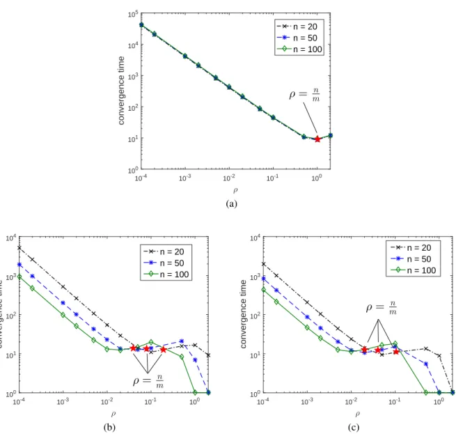
4.3.1 Consensus Error . . . 46 4.3.2 Cyclic Period . . . 47 4.3.3 Convergence Time . . . 47 4.4 Simulations . . . 48 4.4.1 Consensus Error . . . 48 4.4.2 Cyclic Period . . . 50

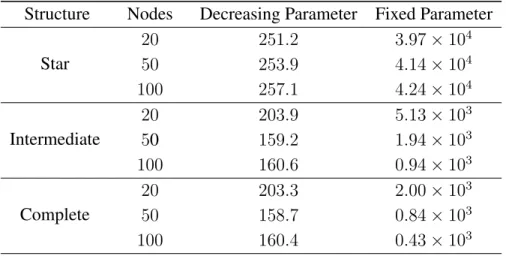
4.4.3 Decreasing Strategy for Parameter Selection . . . 52

4.5 Summary . . . 55

4.6 Proof of Lemma 4.1 . . . 55

4.7 Proof of Theorem 4.1 . . . 57

5 Consensus Based Detection in Sensor Networks via One-bit Communications 62 5.1 Problem and Preliminary . . . 62

5.1.1 Problem Statement . . . 63

5.2 Distributed Average Consensus using One-Bit Communications . . . 68

5.3 Optimal Asymptotic Performance . . . 72

5.3.1 Neyman-Pearson Criterion with Constant Constraint . . . 72

5.3.2 MAP Criterion . . . 75

5.3.3 Neyman-Pearson Criterion with Exponential Constraint . . . 81

5.3.4 Remarks . . . 83 5.4 Non-asymptotic Performance . . . 86 5.5 Simulations . . . 88 5.5.1 Non-asymptotic Performance . . . 88 5.5.2 Convergence Time . . . 90 5.6 Summary . . . 91 5.7 Proof of Theorem 5.5 . . . 92

6 Conclusion and Future Work 97 6.1 Characterization on Convergence Time . . . 97

6.2 General Convex Functions . . . 98

6.3 Online/Sequential Setting for Distributed Detection . . . 98

References 99

Vita 105

3.1 Iterative error versus iterations where each plotted value is the average of1000runs. 28 3.2 Consensus error of the four algorithms where ∆ = 1and the plotted values are

the average of100 runs; (a) fixingn = 50 and varyingm ∈ [49,1225], (b) fixing

m= 400and varyingn ∈[29,399], (c) fixing 2_nm = 10and varyingn∈[20,200]. . 30 3.3 Convergence time of the four algorithms where ∆ = 1 and the plotted values

are the average of 100 runs; (a) n = 50 and m ∈ [49,1225], (b)m = 400and

n ∈[29,399], (c) 2_nm = 10andn∈[20,200]. . . 31 3.4 Consensus error of PQDQ-CADMM with different quantization resolutions, i.e.,

∆∈ {0.02,0.1,0.5,2.5}, forn = 50andm∈[49,1225]; each plotted value is the average of100runs. . . 32 3.5 Number of cyclic cases in104 _{trials. . . . 33}

4.1 Trajectories of EBQ-CADMM;n = 50, m = 100, L = n₂, ∆ = 1,ρ = 0.5, and

ri ∼(n, n2). . . 49

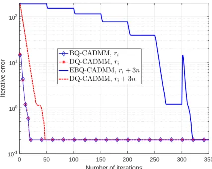
4.2 Iterative errors of BQ-CADMM, EBQ-CADMM, and DQ-CADMM.n = 75,m = 200,L= n₂,∆ = 1,ρ= 0.5, andri ∼ N(0, n2). . . 50

4.3 Empirical probability of cyclic case of BQ-CADMM in10,000runs;ri ∼ N(0,100)+

r0 withr0 ∼ N(0,25),L= 30and∆ = 1. (a) star graph, (b) randomly generated graph withm=l(n+2)(₄n−1)m, (c) complete graph. . . 51

10,000runs;ri ∼ N(0,100) +r0withr0 ∼ N(0,25),L= 30and∆ = 1. (a) star graph, (b) randomly generated graph withm =l(n+2)(₄n−1)m, (c) complete graph. . 53

5.1 Error probability of Monte Carlo simulations for the Gaussian example; the num-ber of trials for each plotted value is105_{. . . . 89} 5.2 Number of cyclic cases in105 _{trials for the Gaussian example. . . . 89} 5.3 Convergence time of BQ-CADMM for the Gaussian example withπ1 = 0.5; each

plotted value is the average of2,000runs. . . 91 5.4 Convergence time of BQ-CADMM using decreasing parameter strategy for the

Gaussian example withπ1 = 0.5; each plotted value is the average of2,000runs. . 92

C

HAPTER

1

I

NTRODUCTION

Collaborative in-network processing is a major tenet in the fields of control, signal processing, information theory, and computer science. Agents operating in a coordinated fashion can gain greater efficiency and operational capability than those perform solo missions. A fundamental concern in such systems is the consensusproblem which aims to reach an agreement among all agents. Of particular interest is thedistributed average consensus which computes the global av-erage of agents’ data through only local computations and communications. Originating from distributed computation and decision-making [1, 2], distributed average consensus has arisen in various recent applications. For example, coordination for autonomous mobile agents [3–5] can often be formulated as a consensus average problem and is key to unmanned aerial vehicle (UAV) formation control and collision avoidance. Another application is in distributed hypothesis testing over a connected network [6, 7] where independently and identically distributed (i.i.d.) observa-tions are collected across the network. Invariably, global log-likelihood ratio (LLR) is a sufficient statistic for all optimal detectors and with i.i.d. data, such a global LLR is simply the average of all local LLRs. Load balancing [8] is yet another example where task assignment across processors needs to equalize processing requirement and be completed in a timely manner.

Distributed averaging algorithms refer to iterative algorithms that aim to achieve the average consensus in a distributed manner. These algorithms are extremely attractive for large scale

net-works characterized by the lack of centralized access to information. They are also energy efficient and enhance the survivability of the networks compared with fusion center based processing. How-ever, real networks can only allow messages with limited length to be transmitted between agents due to physical constraints such as limited bandwidth, sensor battery power, and computing re-sources. When a real value is sent from an agent to its neighbors, this value will be truncated or compressed and it is normally assumed that agents can reliably transmit onlyquantized data. The average consensus problem with this quantization constraint is referred to asquantized consensus

in the literature [9], and iterative algorithms that can work with this constraint is called quantized consensus algorithms. This dissertation focuses on developing efficient quantized consensus algo-rithms for networked applications and in particular, consensus based detection in large scale sensor networks.

1.1

Literature Review

1.1.1

Distributed Averaging and Quantized Consensus Algorithms

There are three widely used methods for solving distributed average consensus problems. A clas-sical approach is to update the state of each node with a weighted average of values from neigh-boring nodes [10–12]. The matrix, consisting of the weights associated with the edges, is chosen to be doubly stochastic to ensure convergence to the average. Another method is a gossip based algorithm, initially introduced in [1] for consensus problems and further studied in [9, 13, 14], among others. The third approach is to employ the alternating direction method of multipliers (ADMM) which is an iterative algorithm for solving convex problems and has received much at-tention recently (see [15] and references therein). The idea is to formulate the data average as the solution to a least-squares problem and manipulate the ADMM updates to derive a distributed algorithm [16–18]. Viewed from this point, applying distributed gradient descent or distributed (ac-celerated) proximal-gradient methods to the least-squares problem results in the classical method or some variants.

In the most ideal case where agents are able to send and receive real values with infinite pre-cision, the three methods can all lead to the desired consensus at the average. When quantization is imposed, however, these methods do not directly apply. A well studied approach for quantized consensus is to use dithered quantizers which add noises to agents’ variables before quantiza-tion [19]. By imposing certain condiquantiza-tions, the quantizaquantiza-tion error sequence becomes i.i.d. and is also independent of the input sequence. The classical approach and the gossip based algorithm then yield the almost sure consensus at a common but random quantization level with the expectation of the consensus value equal to the desired average [20–22]. To the best of our knowledge, there have been no existing results on the ADMM based method for quantized consensus. Nevertheless, since the quantization error of dithered quantizer is zero-mean and has a bounded variance, we can immediately extend the results in [17, 18] to quantized consensus (see Chapter 3.2). That is, the ADMM based method using dithered quantization leads to the consensus at the data average in the mean sense whose variance converges to a finite value.

Meanwhile, studies on distributed average consensus with deterministic quantizers have been scarcely reported. Deterministic quantization makes the problem much harder to deal with as the error terms caused by quantization no longer possess tractable statistical characteristics [20, 21]. The authors in [12] show that the classical approach, where a quantization rule that rounds the values down is adopted, converges to a consensus with an error from the average depending on the quantization resolution, the number of agents, the agents’ data, and the updated weights of each agent. In [23], quantized consensus is formulated as a feedback control design problem for coding/decoding schemes. With an appropriate scaling function and carefully chosen control gain when some spectral properties of the Laplacian matrix of the underlying fixed undirected graph is known in advance, the proposed protocol with rounding quantizer is shown to achieve the exact average consensus asymptotically. A recent result of [24] indicates that this approach, with appropriate choices of the weights, reaches a quantized consensus close to the average in finite time or leads all agents’ variables to cycle in a small neighborhood around the average; in the latter case, however, a consensus is not guaranteed. The gossip based algorithms in [22] and [9]

have similar results to those of the classical approach with probability one (or at least with high probability), where the randomness is from the random selection of the edge at each iteration. The ADMM based algorithms for deterministically quantized consensus, however, have not yet been explored.

1.1.2

Consensus Based Detection

An application of distributed average consensus lies in distributed detection in sensor networks, where the local data are LLRs of local observations and their average, called average LLR, is sufficient to achieve the optimal detection performance under broad conditions [25–31]. Different from canonical structures where there is a fusion center accessing information, consensus based detection deals with network inference problems in the absence of any fusion center [6, 7, 32–36]. Sensors iteratively exchange information with their neighbors to arrive at a consensus decision based on some consensus rules.

Practical channels, especially those employed in large scale sensor networks, are subject to strict bandwidth and resource limits, and again sensors are normally assumed to be able to reliably transmit only quantized data. Of particular interest is the extreme case where each sensor can only send one-bit information. Tsitsiklis established in [30] the optimality of identical likelihood ratio quantizers in such a setting for a canonical fusion network with communications allowed from the sensor to the fusion center (i.e., no consensus type iterations). The resulting decay rate is typically lower than the centralized one under the Neyman-Pearson or maximuma posteoriori

(MAP) criteria. For the tandem network, it was shown in [31] that using a one-bit quantizer at each sensor can never achieve an exponential decay rate of the error probability under the MAP criterion. To the best of our knowledge, there is no asymptotic result on consensus based structures using one-bit quantizer at each node. As such, it isa prioriunknown whether one-bit quantization in a general connected network that allows iterative communications can achieve exponentially decaying error probability and what would be the optimal exponent if exponentially vanishing error probability is feasible. Note that if nodes have perfect knowledge of global network topology, one

can construct schemes that utilize source coding ideas to attain the same optimal error exponent as in the centralized setting. This, however, is not realistic in most applications where nodes only have knowledge of their directly connected neighbors.

1.2

Motivations

1.2.1

Consensus Error Bound in Large Networks

We may roughly divide existing quantized consensus algorithms into two types according to their convergence results: one has asymptotic convergence to the exact average for each agent (e.g., [17,18,20–23]) and the other reaches a consensus within finite iterations at a cost of consensus error from the desired average (see [12, 22]). The second type of algorithms usually adopt deterministic quantizers and are preferred in situations where consensus needs reaching in finite time, e.g., a team of members may have to reach some agreement within finite time and can afford some suboptimal consensuses. Existing algorithms of the second type, however, have increasing consensus error bounds in the range of agents’ data and the size of network, which may not be satisfactory enough in large scale networks. This motivates us to develop quantized consensus algorithms that are more favored in large networks.

1.2.2

Finite-bit Communications

We notice that the quantizers in most existing works are still of infinite bits since the quantizer output has unbounded range and infinite quantization levels. To our best knowledge, in order to employ finite-bit communications per iteration, all existing works using uniform quantizers assume that agents’ data are bounded and the bound is known a priori, which is in general very restrictive and prohibits many networked applications. For example, consensus based detection has agents’ data being local LLRS that can be arbitrarily large for common distributions, e.g., Gaussian distributions. Naively truncating the agents’ data, however, has no consensus accuracy

guarantee. This is indeed the reason that there is no asymptotic characterization for consensus based detection using finite-bit data communications. Thus, quantized consensus algorithms using bounded quantizer for possibly unbounded data not only reduce the cost of data communications but also induce potential applications.

1.2.3

Asymptotically Optimal Detection in Sensor Networks

Sensor networks in today’s applications can be very large. In the scenario of distributed detection, this implies the error exponent, assuming for now that error probabilities can decay exponentially in the size of networks, matters. Consensus based detection in sensor networks has been widely studied in [6, 7, 32–36] where exponential decay of error probabilities are indeed achieved in either online or offline settings. However, not only the error exponent is suboptimal to the centralized one in general, but also the data communicated among linked sensors are of infinite levels and hence of infinite bits. Simply using truncation to achieve finite-bit data communications do not have the same exponential decay results. Therefore, it is unknown if using finite-bit communications can lead to exponential decaying error probabilities, not to mention the optimal error exponent in centralized settings where all the observations are available for decision making.

On the other hand, the work of [30, 31] indicates that one-bit communications in general are not sufficient to achieve the optimal exponential decay of error probabilities in fusion center based schemes. This is not surprising as the information is highly compressed: each node send only one-bit information to the fusion center in parallel schemes or to the serial node in tandem schemes. In consensus based detection, while nodes can only communicate with their direct neighbors, the communications are allowed numerous times. In this sense, it might be possible that a quantized consensus approach can asymptotically achieve the optimal centralized error exponent using only finite-bit communications per iteration.

1.3

Contributions and Organization

Driven by the above facts, this dissertation aims to develop efficient quantized consensus algo-rithms for large scale networks and to apply them to distributed detection in connected sensor net-works. We consider bidirectional connected networks with fixed topology and the quantizers used for data communications are uniform. Nodes can only communicate with their direct neighbors in a synchronous manner. The ADMM has been known to be an efficient algorithm for large scale op-timizations and used in various applications such as regression and classification [15]. Moreover, the work of [37–39] validates the fast convergence of the ADMM and [17, 18] demonstrates the resilience of the ADMM to noise, link failures, etc. Also noticing that probabilistic quantization introduces additional randomness on the consensus result, making it difficult to achieve the optimal exponential decay, we therefore develop quantized consensus algorithms based on the ADMM and deterministic quantization schemes.

The contributions are summarized as follows:

• We study the effects of dithered and deterministic quantizations on an ADMM based dis-tributed averaging algorithm. With probabilistic quantization, this algorithm yields linear convergence to the desired average in the mean sense with a bounded variance. When deter-ministic quantization is employed, it either converges to a consensus or cycles with a finite period after a finite-time iteration. In the cyclic case, local quantized variables have the same sample mean over one period and hence each node can also reach a consensus. We also obtain an upper bound on the consensus error which depends only on the quantization resolution and the average degree of the network. A two-stage algorithm is proposed which combines both probabilistic and deterministic quantizations. Simulations show that the two-stage algorithm, without picking small algorithm parameter, has consensus errors that are typically less than one quantization resolution for all connected networks where agents’ data can be of large variance and magnitudes. These results have been reported in [40–42].

on agents’ data) is known, we use finite-bit bounded quantizers to meet the communication constraint. We show that all the agent variables either converge to the same quantization level or cycle around the data average with the same sample mean over one period after a finite-time iteration. An error bound for the consensus value is obtained which turns out to be the same as that of using the unbounded deterministic quantizer, provided that the ADMM step size is small enough. We then study the effect of the algorithm parameter on our algorithms and propose a decreasing strategy for the parameter selection only using the number of agents and the number of edges in order to accelerate the algorithm with certain consensus accuracy guarantee. This part is from the work of [43, 44].

• We apply the ADMM based quantized consensus algorithm with finite-bit bounded quan-tization to distributed detection in connected sensor networks where each node can only exchange information with its direct neighbors. We establish that, by employing an identical one-bit quantizer for local information exchange, each node can achieve the optimal asymp-totic performance of centralized detection; in particular, each node has its detection error probability decay exponentially with Chernoff information and Kullback-Leibler divergence as error exponents under the maximuma posteriori (MAP) criterion and Neyman-Pearson criterion with constant constraint, respectively. In addition, we examine non-asymptotic per-formance of the proposed approach and show that the type-I and type-II error probabilities at each node can be made arbitrarily close to the centralized ones simultaneously when a continuity condition is satisfied. These results are based on the work of [45, 46].

The rest of this dissertation is organized as follows. Chapter 2 reviews the application of the ADMM to distributed average consensus. Based on this distributed averaging algorithm, we de-velop quantized consensus algorithms using unbounded uniform quantizers in Chapter 3 and using finite-bit uniform quantizers in Chapter 4. In Chapter 5, we apply the proposed algorithm to dis-tributed detection where only one-bit communication between linked nodes at each iteration is allowed. Chapter 6 concludes the dissertation and discusses several future research directions.

1.4

Notations

We use two definitions of rate of convergence for an iterative algorithm. A sequence xk, where the superscriptkstands for time index, is said to converge Q-linearlyto a pointx∗ if there exists a numberυ ∈ (0,1)such thatlimk→∞

kxk+1_−x∗_k

kxk_−x∗_k = υ withk · k being a vector norm. A sequence

yk _{is said to convergeR-linearlyto y}∗

if for allk, kyk_−y∗_{k ≤ kx}k_−x∗_k

wherexk _converges

Q-linearly tox∗.

We use 0 (without subscript) to denote the all-zero column vector whose dimension can be decided from the context. 1K is the K-dimensional all-one column vector; 0K and IK are the

K×K all-zero and identity matrices, respectively. Notation⊗denotes the Kronecker product and

kxk2 denotes the Euclidean norm of a vectorx. Forx ∈ R, dxeis the ceiling function onx, i.e.,

the smallest integer that is greater than or equal tox. Given a positive semidefinite matrixGwith proper dimensions, the G-norm of x is kxkG =

√

xT_{Gx. For a real symmetric matrix L} n×n,

denote its eigenvalues in the ascending order asλ1(L) ≤ λ2(L) ≤ · · · ≤ λn(L). For any matrix

C

HAPTER

2

R

EVIEW OF THE

ADMM

FOR

D

ISTRIBUTED

A

VERAGE

C

ONSENSUS

This chapter briefly reviews consensus ADMM (CADMM) for distributed average consensus where agents can communicate real data of infinite precision, aiming to provide a good under-standing of how the ADMM works and performs in the distributed setting. We start with the network model that is used throughout this dissertation.

2.1

Network Model

Consider a connected network of n agents which are bidirectionally connected bym edges (and thus 2m arcs). We describe this network as a symmetric directed graph Gd = {V,A} or an

undirected graph Gu = {V,E}, where V is the set of vertices with cardinality |V| = n, A

is the set of arcs with |A| = 2m and E is the set of edges with |E| = m. Define the ori-ented incidence matrix M− ∈ Rn×2m with respect to Gd as follows: [M−]i,l = 1 if the lth

arc leaves agent i, [M−]i,l = −1 if the lth enters agent i, and [M−]i,l = 0 otherwise. The

unoriented incidence matrix M+ ∈ Rn×2m is defined by setting [M+]i,l = |[M−]i,l|. Denote

L+= 1₂M+M+T which are respectively the signed and signless Laplacian matrices with respect to

Gu. ThenW = 1₂(L−+L+) =diag{|N1|,|N2|, . . . ,|Nn|}is the degree matrix related toGu, i.e.,

a diagonal matrix with the(i, i)-th entry being|Ni|and other entries being0.

The following lemma states useful properties about the connected network.

Lemma 2.1( [47, 48]). Given a connected network, we have that

a) L−is positive semidefinite and0 = λ1(L−)< λ2(L−)≤λ3(L−)≤ · · · ≤λn(L−). L−b=0

if and only ifb ∈ C(1n)with1nbeing the all-one vector of dimensionn.

b) L+is positive semidefinite andλn(L+)>0.

c) C(M−) = C(L−). For every α ∈ C(L−), there exists a unique β ∈ C(M−T) such that α=M−β.

2.2

The ADMM and Consensus ADMM

The ADMM applies in general to the convex optimization problem in the form of

minimize y1,y2

g1(y1) +g2(y2)

subject to C1y1+C2y2 =c,

(2.1)

wherey1andy2 are optimization variables,g1andg2are convex functions, andC1y1+C2y2 =c is a linear constraint ony1 andy2. The ADMM solves a sequence of subproblems involvingg1 andg2 one at a time and iterate to converge under mild conditions, e.g.,g1 andg2are proper closed convex functions and the Lagrangian of (2.1) has a saddle point [15].

CADMM is obtained by applying the ADMM to minimizing the sum of several convex func-tions in a distributed manner. Letfi :Rd→R, wheredis a positive integer, denote a convex local

use only local computation and communication to find ˜ x∗ = arg min ˜ x n X i=1 fi( ˜x). (2.2)

To obtain the CADMM, we rewrite the above problem in the ADMM form as:

minimize {xi},{zij} n X i=1 fi(xi) subject to xi =zij,xj =zij,∀(i, j)∈ A, (2.3)

wherexi ∈ Rdis the local copy of the common optimization variablex˜at agent iandzij ∈ Rd

is an auxiliary variable imposing the consensus constraint on neighboring agents i and j. This consensus constraint ensures the consensus to be achieved over the entire network, i.e., xi =

xj for all i, j ∈ V, which in turn guarantees that (2.3) is equivalent to (2.2). Further definex ∈

Rnd as a vector concatenating all xi, z ∈ R2md as a vector concatenating all zij, and f(x) =

Pn

i=1fi(xi). Then (2.3) can be written in a matrix form as

minimize

x,z f(x) +g(z)

subject to Ax+Bz =0,

(2.4)

whereg(z) = 0, and0 is a column vector with proper dimensions and all entries being0. Here B = [−I2md;−I2md] with I2md being a 2md ×2md identity matrix and A = [A1;A2] with A1,A2 ∈R2md×nd. If(i, j)∈ Aandzij is theqth block ofz, then the(q, i)th block ofA1and the

(q, j)th block ofA2 areId; otherwise the corresponding entries are0d.

With this matrix form, we are ready to write out the ADMM updates. The augmented La-grangian of (2.4) is Lρ(x,z,λ) =f(x) +hλ,Ax+Bzi+ ρ 2kAx+Bzk 2 2, (2.5)

parameter. At iteration k+ 1, the ADMM first obtains xk+1 _{by minimizing L}

ρ(x,zk,λk), then

calculateszk+1by minimizingLρ(xk+1,z,λk)and finally updatesλk+1usingxk+1andzk+1. The

updates are

x-update:∂f(xk+1) +ATλk+ρAT(Axk+1+Bzk) =0,

z-update: BTλk+ρBT(Axk+1+Bzk+1) =0,

λ-update: λk+1−λk−ρ(Axk+1+Bzk+1) =0,

(2.6)

where∂f(xk+1_{)is a subgradient off atx}k+1_{. Thex-update andz-update can also be viewed as} proximal updates; see [49].

A nice property of the ADMM, known asglobal convergence, states that the sequence(xk,zk,λk)

generated by (2.6) has a single limit point(x∗,z∗,λ∗)which is a primal-dual solution to (2.5), as stated in Lemma 2.2.

Lemma 2.2(Global convergence of the ADMM [15,37,39]). Assume that local objective functions

fi are proper closed convex functions and that the minimum of (2.2) is attainable. For any initial

valuesx0 _∈

Rnd,z0 ∈R2mdandλ0 ∈R4md, the update in (2.6) yields that

xk→x∗, zk →z∗, andλk →λ∗ask → ∞,

where(x∗,z∗,λ∗)is a primal-dual solution to (2.5).

While (2.6) provides an efficient centralized algorithm to solve (2.2), it is not clear whether (2.6) can be carried out in a distributed manner, i.e., data exchanges only occur within neighboring nodes. Interestingly, Lemma 2.2 states that convergence for the ADMM is guaranteed regardless of initial valuesx0_,z0 _andλ0_{; there indeed exist initial values that decentralize (2.6). Initialize} β0 _=−γ0_andz0 ₌ 1

2(M

T

the updates in (2.6) lead to the following iterative updates: ∂fi(xki+1) + 2ρ|Ni|xik+1− ρ|Ni|xki +ρ X j∈Ni xk_j −αk_i ! =0, αk_i+1 =αk_i +ρ |Ni|xki+1− X j∈Ni xk_j+1 ! , (2.7) at agenti, whereαk

i ∈Rdis the local Lagrangian multiplier of agenti. The above updates are fully

decentralized as the update ofxk_i+1andαk_i+1only relies on local and neighboring information. We refer to (2.7) as CADMM.

The following theorem states the convergence of CADMM, which follows directly from global convergence of the ADMM.

Lemma 2.3 (Convergence of CADMM [15, 37]). Assume that local objective functions fi are

proper closed convex functions and that the minimum of (2.2) is attainable. Then CADMM is guaranteed to converge for anyx0

i ∈Rd,[α01;α02;· · · ;α0n]∈ C(L−⊗Id), andρ >0: lim k→∞x k i = ˜x ∗_and lim k→∞α k i =α ∗ i, i= 1,2, . . . , n,

where x∗₁ = · · · = x∗_{n ,} x˜∗ and α∗_i are a pair of primal and dual solutions to (2.3), andx˜∗ is optimal to (2.2).

The ADMM and CADMM are also shown to converge linearly when certain convexity assump-tions on the objective funcassump-tionsfi’s are satisfied; see, e.g., [38, 39, 50]. As this dissertation focuses

on distributed average consensus, we only consider the convergence rate result when CADMM is applied to distributed average consensus. This is presented in the next section.

2.3

CADMM for Distributed Average Consensus

Denote by ri ∈ R the measurement at agent i, r the vector that concatenates all ri, and r¯ =

1

n

Pn

by identifying that the average is the unique solution to a least-squares problem, i.e., ¯ r = arg min ˜ x 1 2 n X i=1 (˜x−ri)2.

Therefore, we have the CADMM updates for distributed averaging by plugging infi(˜x) = 1₂(˜x−

ri)2: xk_i+1= 1 1 + 2ρ|Ni| ρ|Ni|xki +ρ X j∈Ni xk_j −αk_i +ri ! , α_ik+1=αk_i +ρ |Ni|xki − X j∈Ni xk_j ! . (2.8)

For ease of presentation, we will use ‘CADMM’ to refer to the above updates and ‘original CADMM’ for the updates in (2.7) where local objectives are general convex functions. We can further write (2.8) in a matrix form as

xk+1 = (In+ 2ρW)−1(ρL+xk−αk+r), αk+1 =αk+ρL−xk+1, or more compactly, sk+1 =Dsk, (2.9) wheresk₌ xk_;αk_;r ,D0 = (In+ 2ρW)−1, and D=        ρD0L+ −D0 D0 ρ2L−D0L+ In−ρL−D0 ρL−D0 0n 0n In        . (2.10)

Following (2.9), we can writeskas

It is thus interesting to investigate howDk _{behaves as k → ∞. From (2.10), a logical approach}

is to study Dk through the structures of L−,L+ and W; fortunately, the convergence property of CADMM provides a simple argument to obtain a rough estimate ofD∞, which, nevertheless, is good enough for our purpose. Note that we also have D∗ = D∞ and s∗ = [x∗;α∗;r] = [x∞;α∞;r] =s∞as the optimum due to the convergence of CADMM. The result is given below

Theorem 2.1. ConsiderDdefined in (2.10). Then

D∗ =        D11 D12 D13 D21 D22 D23 D31 D32 D33        =        0n a11Tn 1 n1n1 T n 0n a21Tn In−_n11n1Tn 0n 0n In        for fixeda1,a2 ∈Rn.

Proof. By Lemma 2.3, we have for anys0 that satisfies the initialization condition,

s∞=        x∞ α∞ r∞        =        x∗ α∗ r∗        =        1nr¯ r−1nr¯ r        .

Recall thats∞=D∞s0. If we fixα0andr0, global convergence implies thats∞=s∗ regardless of the initial value x0_{. Thus D}

i1 = 0n, i = 1,2,3. Similarly, fixing x0 and r0, we must have

D12α0 = D22α0 =0. Sinceα0 is initialized in the column space ofM−M−T = 2L−whereL− is the signed Laplacian matrix of a connected undirected graph,D12andD22must be respectively the products of some vectors a1 anda2 inRn multiplying1Tn such that D12L− = D22L− = 0. Knowing the form ofDj1 andDj2withj = 1,2, we see thatx∞andα∞only depend onr0 =r. Together with the facts thatx∞=x∗has each entry of itself reaching the data averager¯= _n1rT1n

and thatα∞=r−1nr¯for anyr, we validateD13andD23as given in the theorem. The remaining blocks,D32andD33, follow directly from the matrix multiplication.

Given convergence, we now turn our attention to the rate of convergence of CADMM. Recent work of [38, 39] has established the linear convergence of the ADMM. Unfortunately, their results do not apply to CADMM as their conditions are not satisfied here. In [38], the step size of the dual variable update, i.e., ρ in the λ-update of (2.6), need be sufficiently small while CADMM has a fixed step sizeρthat can be any positive number (see Remark 3.3 for further discussion on the choice ofρ). The linear convergence in [39] is established provided that eitherg(z)is strongly convex orBis full row-rank in (2.3). In our formulation, however,g(z) = 0is not strongly convex and B = [−I2m;−I2m] is row-rank deficient. Fortunately, [50, Theorem 1] characterizes the

convergence rate of a vector concatenatingz andβ, which can be used to derive the convergence rate aboutsk. Before stating this result in Theorem 2.2, we futher define

uk =    zk βk    andG=    ρI2m 02m 02m 1_ρI2m   . (2.11)

Theorem 2.2(Linear convergence of CADMM for distributed average consensus [50]). Letx0 _∈

Rnandα0 ∈ C(L−). Thenukconverges Q-linearly tou∗ = [z∗;β∗], withz∗ = 1₂M+1nr¯andβ∗

being the unique vector inC(M−)such thatM−Tβ∗ =r−1nr¯, with respect to theG-norm:

kuk+1−u∗kG ≤ 1 1 +ηku k_−u∗_k G, (2.12) wherekuk+1_−u∗_k G = p (uk+1_−u∗₎T_Guk+1_−u∗_,η=√_{1 +δ−1,µ >1, and} δ= min (µ−1)λ2(L−) µλn(L+) , 2ρλ2(L−) ρ2_λ n(L+)λ2(L−) +µ .

Furthermore,sk_{is R-linearly convergent tos}∗_as

ksk+1−s∗k2 ≤ 1 + p 2ρλn(L−) 1 +η ! kuk−u∗kG. (2.13)

chosen algorithm parameters. These algorithms, however, require the knowledge of an upper bound onri’s in order to select the right algorithm parameters to deal with the bounded

quantiza-tion constraint. In Chapter 4, we will show that the local Lagrangian multipliersαi’s in CADMM

play a key role in handling the bounded quantization.

2.4

Summary

This chapter introduces CADMM for distributed average consensus and its convergence properties. These results will be used to analyze the proposed quantized CADMM algorithms in the following two chapters.

C

HAPTER

3

Q

UANTIZED

C

ONSENSUS BY THE

ADMM:

U

NBOUNDED

Q

UANTIZATION

This chapter considers distributed average consensus subject to quantized communication con-straints. For the present chapter, we do not require the quantizer to be of finite bits. However, if agents’ data are bounded and a bound is known, then truncation can be used before quantization to achieve finite-bit data communications.

3.1

Model of Quantized Communication

To model the effect of quantized communications, we assume that each agent can store and com-pute real values with infinite precision; however, an agent can only transmit quantized data through the channel which are received by its neighbors without any error. The quantization operation is defined as follows. Let∆>0be the quantization resolution. Define the quantization lattice in_R by

Λ ={t∆ :t ∈_Z}.

A (uniform) quantizer is a functionQ:_R→Λthat maps a real value to some point inΛ. Among all unbounded quantizers we consider the following two:

• Probabilistic quantizerQp defined as follows: fory∈[t∆,(t+ 1)∆), Qp(y) =        t∆, with probabilityt+ 1− y ∆, (t+ 1)∆, with probability _∆y −t. (3.1)

• Rounding quantizerQdwhich projectsy ∈Rto its nearest point inΛ:

Qd(y) =t∆, if t− 1 2 ∆< y ≤ t+1 2 ∆. (3.2)

We point out that probabilistic quantization is equivalent to a dithered quantization method (see [20, Lemma 2]) while rounding quantization is one of the deterministic quantization schemes. Through the rest of this dissertation, we mean quantizing each of the entries when the quantizer has a vector input. Definee(y) = Q(y)−yas the quantization error. It is clear that

|ep(y)| ≤∆and |ed(y)| ≤

1

2∆, for anyy∈R. (3.3)

We will investigate how the quantized communication affects CADMM in the following two sections. We remark that the results of probabilistic and rounding quantizations can easily extend to other dithered and deterministic cases, which will be elaborated in Sections 3.2 and 3.3.

3.2

Probabilistic Quantized CADMM (PQ-CADMM)

For ease of presentation, we only study the probabilistic quantization defined in (3.1). The results can be easily extended to any other dithered quantization as the only information used is the first and second order moments of the probabilistic quantizer output, which are common properties among all dithered quantizers. The properties are stated in the following lemma.

Lemma 3.1( [51, Lemma 2]). For everyy∈_R, it holds that E[Qp(y)] =y and E (y− Qp(y)) 2 ≤ ∆ 2 4 .

Furthermore, for any inputsy1 andy2, the quantization errorsep(y1)andep(y2)are independent and identically distributed (i.i.d.), and are independent of the inputsy1andy2 repsectively.

We use the probabilistic quantization to modify the CADMM update (2.8) as

xk_i+1 = 1 1 + 2ρ|Ni| ρ|Ni|Qp xkj +ρX j∈Ni Qp xkj −αk_i +ri ! , αk_i+1 =αk_i +ρ |Ni|Qp xki+1 − X j∈Ni Qp xkj+1 ! . (3.4)

Notice that xk_i is also quantized at its own node for the (k + 1)th update; the reason will be given in Remark 3.5. As illustrated in [17], the above iteration can be interpreted as a stochastic gradient update. Viewed from this point, the quantization operation causesxk_i to fluctuate around the quantization-free updates (2.8). The convergence claims are given in Theorem 3.1.

Theorem 3.1. For any x0 _∈

Rn and α0 ∈ C(L−), the probabilistic quantized CADMM

(PQ-CADMM) iteration (3.4) generatesxk

i, i = 1,2, . . . , n, which converges linearly to the data

aver-ager¯in the mean sense ask → ∞, i.e.,

lim

k→∞E

xk_i

= ¯r, i= 1,2, . . . , n.

In addition, the variance of xk

i converges to a finite value which depends on the quantization

Proof. Taking expectation of both sides of (3.4), we have E[xki+1] = 1 1 + 2ρ|Ni| ρ|Ni|EQp(xki) +ρX j∈Ni EQp(xkj) −_E[αk_i] +ri ! , E[αki+1] =E[α k i] +ρ |Ni|E Qp(xki+1) −X j∈Ni EQp(xkj+1) ! . (3.5)

Noting that Lemma 3.1 implies_EQp(xki)

= _E[xk i]and E Qp(xkj) = _E[xk j], we see that (3.5)

takes exactly the same iterations in the mean sense as CADMM for distributed average consensus. By initializingα0 _∈L

−, we haveE[α0] =α0lies inC(L−), too. The linear convergence ofE[xki]

tor¯is thus ensured due to Theorem 2.2.

Since Lemma 3.1 also indicates the bounded variance of quantization error, the second claim follows directly from [17, Proposition 3].

We notice that the convergence of _E[xk

i] to r¯with bounded variance does not imply that xk

reaches a consensus whenk → ∞. Nevertheless, a simple method fixes this problem. The idea is to calculate the running averagex¯k_i = 1_kPk

l=1x

l

i, k ≥ 1at nodei. Since the variance is bounded,

one can use similar steps as in [17] together with Chebyshev’s inequality to get that x¯k_i → r¯in probability.

3.3

Deterministic Quantized CADMM (DQ-CADMM)

Deterministic quantization is usually much harder to handle as the quantization error is not stochas-tic. Unlike probabilistic quantization, the accumulated error term can blow up; there have been a few methods proposed to counter such difficulties (see [12, 22, 24]), yet the resulting algorithms either do not guarantee a consensus or reach a consensus with an error from the desired average that depends on the number of agents, the quantization resolution, and the agents’ data. To analyze the consensus reaching result, we first find a finite upper bound on the accumulated error term and then utilize the property and the initialization condition of local Lagrangian multipliers .

Let the local dataxk

i be also quantized for the(k+ 1)-th update at nodei. The updates become

xk_i+1= 1 1 + 2ρ|Ni| ρ|Ni|Qd xkj +ρX j∈Ni Qd xkj −αk_i +ri ! , αk_i+1 =αk_i +ρ |Ni|Qd xki+1 − X j∈Ni Qd xkj+1 ! . (3.6)

We can rewriteQd(xki) =xki +ed(xki). Then theαi-update is equivalent to

αk_i+1 =αk_i +ρ |Ni|xki+1− X j∈Ni xk_j+1 ! +ρ |Ni|ed(xki+1)− X j∈Ni ed(xkj+1) ! ,

or written in the matrix form,

αk+1 =αk+ρL−xk+1+ρL−ed(xk+1), (3.7)

where ed(xk+1) denotes the vector concatenating all ed(xki+1). Recalling the CADMM update

(2.9), we can write the matrix form of (3.6) as

sk+1 =D(sk+sk_x) +sk_α (3.8) wheresk x = ed(xk);0;0 andsk α = 0;ρL−ed(xk+1);0

. It is important to note the update above update is deterministic, i.e., given sk1 _{= s}k2 _{that are some states, we must haves}k1+1 _{= s}k2+1_.

The result of (3.6) is characterized in the following theorem.

Theorem 3.2. Consider the deterministic quantized CADMM (DQ-CADMM) iteration (3.6). Let

x0 ∈_Rn_andα0 _{∈ C(L}

−). Then there exists a finite time iterationk0 ≥1such that fork ≥k0, all the quantized variable values

• either converge to the same quantization value:

Qd xk1 =Qd xk2 =· · ·=Qd xkn ,x∗_Q d,

• or cycle around the averager¯with a finite periodT ≥ 2, i.e., Qd xki = Qd xki+T , i = 1,2, . . . , n, and 1 T T X l=1 Qd xk1+l = 1 T T X l=1 Qd xk2+l =· · ·= 1 T T X l=1 Qd xkn+l ,x¯∗_Q d. (3.9)

Furthermore, we have the following error bound forx∗_[Q

d]∈ x∗_Q d,x¯ ∗ Qd : x∗_[Q d]−r¯ ≤ 1 + 4ρm n ∆ 2, (3.10)

where the upper bound is tight if DQ-CADMM converges.

Proof. See Section 3.7.

Remark 3.1. The result that deterministic quantization may lead the average consensus algorithm

to either convergent or cyclic cases is also reported in [24]. Similar to theirs, one can use the history of agents’ variables, e.g., running average, to achieve asymptotic convergence at each node. Different to theirs, while their algorithm can make local variable values close to the true average in cyclic cases without guaranteeing a consensus, our algorithm can reach a consensus but does not make the error arbitrarily small in general.

Remark 3.2. We shall mention that x∗_Q

d or x¯

∗

Qd need not be unique. This is because, unlike CADMM,kuk_−u∗_k

G in DQ-CADMM need not decrease monotonically due to the quantization

that occurs on xk at each update. Note also that practical consensus value does not necessarily meet the error bound and we usually have smaller errors than (3.10) in practice (see simulations). We hence expect better consensuses when(x0_,α0_{)are initialized closer to the ideal optima, which} leads to a two-stage algorithm for quantized consensus in Section 3.4.

Remark 3.3. An interesting observation of our main result is the ADMM parameter ρ. While

a small ρ indicates a small consensus error bound, the current chapter does not quantify how it affects the convergence timek0as well as the cyclic periodT. We do not study the optimal selection

ofρbut simply setρ= 1 for the present chapter. We will discuss the effect ofρin more details in Chapter 4 .

Remark 3.4. Theorem 3.2 for rounding quantization extends straightforward to other

determinis-tic quantizations as the only information used in our proof is the bounded quantization error. In contrast with [9, 12] where the algorithms may fail for some deterministic quantization schemes, e.g., the rounding quantization, our results work for all deterministic quantization schemes as long as a finite quantization error bound is provided.

Remark 3.5. In both PQ-CADMM and DQ-CADMM iterations,xk

i is quantized for the(k+ 1)th

update at nodeieven though nodes can compute and store real values with infinite precision. The reason is to guarantee thatαklies in the column space ofL−and thus the ideal CADMM update

in either PQ-CADMM or DQ-CADMM (cf. Eq. (3.8)) possesses the linear convergence property given in Theorem 2.2. If we do not quantize xk

i at its own node, Theorem 3.1 still holds due to

E[Qp(xki)] =E[xki]while Theorem 3.2 may fail.

3.4

A Two-Stage Algorithm for Quantized Consensus

Let us summarize the two quantized versions of CADMM: PQ-CADMM converges linearly to the data average in the mean sense, but it does not guarantee a consensus within finite iterations; DQ-CADMM, on the other hand, either converges to a consensus or cycles with the same mean of quantized variable values over one period at each node after a finite-time iteration, but results in an error from the true average.

As discussed in Remark 3.2, we can first run PQ-CADMM2Ktimes to obtainx¯i = _K1 P2_kK_=K+1xki,

which is a reasonable estimate ofr¯at node i according to Theorem 3.1. Here K can be chosen such that E[xKi ] is close enough to ¯r when we have the knowledge of agents’ data and the

net-work topology. Otherwise, we can simply pickK =10n log₁₀(_∆1 + 1) + 1max{−log₁₀ρ,1}

which works well in practice, or as large as permitted. Also, α¯i = _K1

P2K

k=K+1αki is a good

esti-mate of α∗_i = ri −¯r, and that α¯ = [ ¯α1; ¯α2;· · · ; ¯αn] = _K1

P2K

condition asαk _{lies in the column space ofL}

−. We can therefore run DQ-CADMM with thisx¯i

andα¯i as initial values. The probabilistic quantized CADMM followed by deterministic quantized

CADMM (PQDQ-CADMM) is presented in Algorithm 3.1.

Algorithm 3.1PQDQ-CADMM for quantized consensus

Require: Initializeρ > 0, K =10n log₁₀(_∆1 + 1) + 1max{−log₁₀ρ,1}

,x0 =0, andα0 =0.

1: fork= 0,1,· · · ,2K−1, every nodeido

xk_i+1 ← 1 1 + 2ρ|Ni|  ρ|Ni|Qp xki +ρX j∈Ni Qp xkj −αk_i +ri  , αk_i+1 ←αk_i +ρ  |Ni|Qp xki+1 − X j∈Ni Qp xkj+1  . 2: end for 3: x2K i ← 1 K P2K l=K+1xli,α2iK ← 1 K P2K l=K+1αli, andk ←2K. 4: repeat 5: every nodeido xk_i+1 ← 1 1 + 2ρ|Ni|  ρ|Ni|Qd xki +ρX j∈Ni Qd xkj −αk_i +ri  , αk_i+1 ←αk_i +ρ  |Ni|Qd xki+1 − X j∈Ni Qd xkj+1  . 6: k ←k+ 1

7: untila predefined stopping criterion (e.g., a maximum iteration number) is satisfied.

3.5

Simulations

This section investigates the performance of DQ-CADMM and PQDQ-CADMM via numerical examples. To construct a connected graph withnnodes andmedges, we first generate a complete graph consisting ofnnodes, and then randomly remove n(n₂−1) −medges while ensuring that the

network stays connected. Set∆ = 1throughout this section and assume that agents’ data have very high variances in large networks, e.g., letri ∼ N(0, n4). Throughout the rest of this dissertation,

the average simulated result is taken with respect to both graph and agents’ data; that is, both graph and agents’ data are randomly generated at each run.

3.5.1

Performance Comparison

We compare our algorithms with those that use deterministic quantization to reach a consensus, i.e., the gossip based method in [22] and the classical method in [12]. The simulation settings are

• PQDQ-CADMM: Setρ= 1.

• DQ-CADMM: Setρ= 1,x0 _=0andα0 _=0.

• Gossip based method: We randomly pick one edge inA and perform the updating, i.e., if

(i, j)∈ Ais chosen, thenxk_i+1 =xk_j+1 = 1₂ Qd(xki) +Qd(xkj)

.

• Classical method: LetW denote the weight matrix of the graphGd={V,A}. The updating

rule is then given byxk+1 _{= WQ}

rd(xk)where the subscript Qrd(·) denotes the rounding

down quantization. We utilize the Metropolis weights defined in [52]:

Wij =                  (1 + max{|Ni|,|Nj|})−1, (i, j)∈ A, 1−P k∈NiWik, i=j, 0, otherwise.

We simulate a connected network withn = 50nodes andm = 500edges. Define the iterative error askQ(xk₎₋₁

nr¯k2/

√

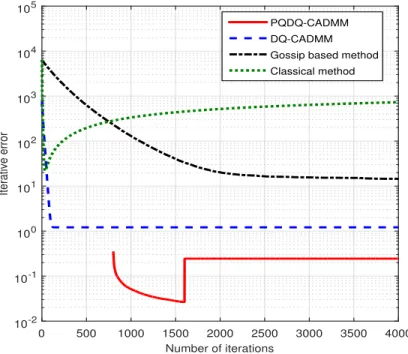
n whereQ(·)denotes the quantization scheme in the respective algo-rithms. Plotted in Fig. 3.1 is the iterative error with each value being the average of1000runs (the iterative error iskx¯k−1nr¯k2 for the PQ-CADMM part of PQDQ-CADMM). Note that we start the plot of PQDQ-CADMM from the (K + 1)-th iteration as its first K iterations are used only

to reach a neighborhood of ¯r; at the (2K + 1)-th iteration, Qd x2K+1

is updated based on the running average of the(K+ 1)-th iteration to the2K-th iteration. The figure indicates that all the four algorithms converge to a consensus at one of the quantization levels. The average consensus error of DQ-CADMM is1.21, which is much smaller than the upper bound (1₂ + 2_nm)∆ = 20.5. One can also see that PQDQ-CADMM converges almost immediately after the2K-th iteration.

Number of iterations 0 500 1000 1500 2000 2500 3000 3500 4000 Iterative error 10-2 10-1 100 101 102 103 104 105 PQDQ-CADMM DQ-CADMM Gossip based method Classical method

Fig. 3.1: Iterative error versus iterations where each plotted value is the average of1000runs.

Consensus error: In Fig. 3.2a we fix n = 50 and vary m until the graph is complete. The gossip based method and the classical method have decreasing consensus errors as m increases. The consensus error of DQ-CADMM, however, becomes larger as the average degree and therefore the error bound increase. PQDQ-CADMM has the smallest consensus error whose average of100

runs is less than 0.40for all m. We then fix m = 400 and let n vary. Fig. 3.2b shows that the gossip based method and the classical method have increasing consensus errors as n increases. The consensus error of DQ-CADMM, on the contrary, decreases whennbecomes larger. PQDQ-CADMM also has the smallest consensus error in this case. In the last setting we fix the average degree 2_nm = 10while varying n. The classical method and the gossip based method then both

have increasing consensus errors whennand thus the range of agents’ data increase. The consensus error of DQ-CADMM is relatively small compared with the upper bound(0.5 +2_nm)∆ = 10.5and decreases whennbecomes larger. The proposed PQDQ-CADMM algorithm still has the smallest consensus error whose average of100runs is less than0.2for alln.

We conclude that the consensus error of the gossip based method and the classical method depends on the average degree of the graph as well as the range of agents’ data. Note that their consensus errors can be extremely large for a sparsely connected graph. DQ-CADMM has an increasing consensus error when the average degree increases while PQDQ-CADMM performs almost the same for all network structures in terms of the consensus error.

Convergence time: We study the convergence time of the four algorithms via numerical exam-ples in Fig. 3.3. Since the gossip based method involves only one edge and the other three methods utilize all the edges at each iteration, we plot also the quotient of the convergence time of the gos-sip based method divided by the number of edges, namely, Gosgos-sip based method adjusted, in the figure.

In Fig. 3.3a, the gossip based method and the classical method converge slower as the graph becomes sparser. When the average degree is fixed, they have longer convergence time as n in-creases. Therefore, the convergence time of the gossip based method and the classical method is also affected by the average degree of the graph and the range of agents’ data. Different from the gossip based and classical methods, we see in Fig. 3.3a that the convergence time of DQ-CADMM increase as the graph becomes denser. In Fig. 3.3b and Fig. 3.3c, however, the convergence time also increases while the graph becomes sparser, which is possibly because of the increased distance between starting variable values and optimal variable values. For PQDQ-CADMM, we observe that the significant portion of its convergence time is spent on achieving an approximate estimate of r¯, i.e., running PQ-CADMM with 2K iterations. With good starting points, DQ-CADMM converges almost immediately.

Number of edges 200 400 600 800 1000 1200 Consensus error 10-1 100 101 102 103 PQDQ-CADMM DQ-CADMM Gossip based method Classical method (a) Number of nodes 50 100 150 200 250 300 350 400 Consensus error 10-1 100 101 102 103 104 PQDQ-CADMM DQ-CADMM Gossip based method Classical method (b) Number of nodes 20 40 60 80 100 120 140 160 180 200 Consensus error 10-1 100 101 102 103 104 PQDQ-CADMM DQ-CADMM Gossip based method Classical method

(c)

Fig. 3.2: Consensus error of the four algorithms where ∆ = 1 and the plotted values are the average of100runs; (a) fixingn= 50and varyingm∈[49,1225], (b) fixingm= 400and varying

Number of edges 200 400 600 800 1000 1200 Convergence time 10-1 100 101 102 103 104 105 PQDQ-CADMM DQ-CADMM Gossip based method Classical method Gossip based method adjusted

(a) Number of nodes 50 100 150 200 250 300 350 400 Convergence time 100 101 102 103 104 105 106 107 PQDQ-CADMM DQ-CADMM Gossip based method Classical method Gossip based method adjusted

(b) Number of nodes 20 40 60 80 100 120 140 160 180 200 Convergence time 100 101 102 103 104 PQDQ-CADMM DQ-CADMM Gossip based method Classical method Gossip based method adjusted

(c)

Fig. 3.3: Convergence time of the four algorithms where∆ = 1 and the plotted values are the average of100runs; (a)n = 50andm ∈ [49,1225], (b)m = 400andn ∈[29,399], (c) 2_nm = 10

3.5.2

Different Quantization Resolutions

We next consider the effect of the quantization resolution on PQDQ-CADMM. Fig. 3.4 plots con-sensus errors of PQDQ-CADMM withn = 50andm ∈ [49,1225]for∆ ∈ {0.02,0.1,0.5,2.5}. The consensus error tends to increase on the average as the quantization resolution becomes larger, which is not surprising since a coarse quantization indicates a higher loss of information at each update. We then calculate the ratio of the consensus error to the quantization resolution: the plot-ted values, which are the averages of100 runs, all lie in (0.227∆,0.337∆)and the variances are less than 0.051. Moreover, the convergence time of each quantization resolution has a mean of

(2K+ 2.1)iterations and a variance less than0.0008, which coincides with our previous analysis that PQDQ-CADMM converges immediately after the first2K iterations.

Numer of edges 200 400 600 800 1000 1200 Consensus error 10-3 10-2 10-1 100 ∆=0.1 ∆=0.5 ∆=2.5 ∆=0.02

Fig. 3.4: Consensus error of PQDQ-CADMM with different quantization resolutions, i.e., ∆ ∈ {0.02,0.1,0.5,2.5}, forn = 50andm∈[49,1225]; each plotted value is the average of100runs.

3.5.3

Cyclic Case

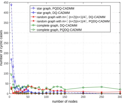
While we prove that DQ-CADMM either converges or cycles in Theorem 4, we note the above numerical examples all lead to reach convergence results. Indeed, the proposed deterministic al-gorithms, DQ-CADMM and PQDQ-CADMM, converges in most cases as shown by the following simulation. For connected networks with n nodes, we consider star graph which has the small-est average degree, randomly generated graph that has intermediate average degree, and complete graph that has the largest average degree. The result is given in Fig. 3.5 where they-axis represents the number of cyclic cases in104 trials. Clearly, DQ-CADMM and PQDQ-CADMM with fixed parameterρ= 1converge in most cases, particularly with large networks. We will study the cyclic case in more details in Chapter 4.

0 50 100 150 200 250 300 number of nodes 0 50 100 150 200 250 300 350 400 450

number of cyclic cases

star graph, PQDQ-CADMM star graph, DQ-CADMM

random graph with m=⌈ (n+2)(n+1)/4⌉, DQ-CADMM random graph with m=⌈ (n+2)(n+1)/4⌉, PQDQ-CADMM complete graph, DQ-CADMM

complete graph, PQDQ-CADMM

3.6

Summary

In this chapter, we propose two quantized versions of CADMM: PQ-CADMM and DQ-CADMM. PQ-CADMM converges linearly to the data average in the mean sense, but it does not guarantee a consensus within finite iterations. DQ-CADMM, on the other hand, either converges to a consensus or cycles with the same mean of quantized variable values over one period at each node after a finite-time iteration but results in an error from the true average. While deterministic quantization is somewhat unfavorable due to the cyclic behavior, a notable fact is that there is no randomness involved. We believe that this property will be useful to some applications, e.g., consensus based detection using one-bit communications as discussed in Chapter 5.

3.7

Proof of Theorem 3.2

Proof. We prove that DQ-CADMM either converges or cycles after a finite-time iteration and then use this fact to derive the error bound.

We see from (3.7) thatαkmust lie in the column space ofL−ifα0 is initialized in the column space ofL−. Following (3.8), we have

sk=D(sk−1 +sk_x−1) +sk_α−1 =D D(sk−2+s_xk−2) +sk_α−2 +Dsk_x−1+sk_α−1 =· · · =Dks0+ k X i=1 Disk_x−i+ k−1 X j=0 Djsk_α−1−j ! . (3.11)

The first term is simply the ideal CADMM update which converges to a finite value. We will show that the accumulated error term Pk

i=1Disk −i x + Pk−1 j=0Djsk −1−j

α is bounded and hence that sk

is bounded. Notice that Disk_x−i is the i-th update of CADMM with the initial value sk_x−i. Let ul_k−i = [z_kl_−i;β_kl_−i]be the vector that concatenates the primal and dual variables in the ADMM

iteration (2.6), with initial valuesz0 k−i = 1 2M T +e k−i d andβk0−i =0corresponding toskx = [ekd;0;0].

WithGdefined in (2.11), we obtain

ku0_k−ik2 G =ρ 1 2M T +e k−i d 2 2 ≤ 1 4ρ2λn(L+)ke k−i d k 2 2 ≤ 1 8ρn∆ 2 λn(L+)(M+),

where the last inequality is from (3.3). Since Theorem 2.1 indicates the form of D∗, we get D∗sk−i x = 0, i.e., x ∗ k−i = 0 andα ∗ k−i = 0. Therefore, u ∗ k−i = [z ∗ k−i;β ∗ k−i] = 0 from Lemma

2.1 and the fact thatz_k∗_−i = 1₂MT

+x∗k−i. Noting also that the initializationzk0−i andβ0k−i meet the

condition of Theorem 2.2, we thus have

kDisk_x−ik2 =k(Di−D∗)skx−ik2 (a) ≤ 1 + r ρ 1 +δ2λn(L−) kui_k−₋1_i−u∗_k−ikG (b) ≤ 1 4 1 + r ρ 1 +δ2λn(L−) r 1 1 +δ !i−1 p 2ρnλn(L+), (3.12)

where(a)and(b)are due to Theorem 2.2 together with the fact thatu∗_k−i =0. Similarly, we have forj ≥1, kDjsk_α−1−jk2 ≤ 1 4 1 + r ρ 1 +δ2λn(L−) r 1 1 +δ !j−1 ∆σmax(M−) √ ρn, (3.13) and whenj = 0, kDjsk_α−1−jk2 =kskα−1k2 ≤ 1 4ρ∆ p 2nλ(L−). (3.14)

Therefore, k X i=1 Disk_x−i+ k−1 X j=0 Djsk_α−1−j 2 ≤ k X i=1 kDisk_e−ik2+ k−1 X j=0 kDjsk_α−1−jk2 ≤ ksk_α−1k2+ k X i=1 kDisk_e−ik2+kDiskα−1−ik2 (a) ≤ 1 4ρ∆ p 2nλ(L−) + 1 + r ρ 1 +δ2λ(L−) × 1 4∆ p ρNp2λ(L−) + p 2λ(L+) _Xk i=1 r 1 1 +δ !i−1 (3.15)

where(a)is from (3.12)-(3.14). Then (3.15) must be finite fork = 1,2, . . . ,as δ > 0, and thus sk _{is bounded. An important fact from (3.8) is that the update of s}k+1 _{and hence s}k+1

x is fully

determined bysk_+sk

x due to the deterministic quantization and the CADMM update. Recalling

thatksk

xk2 =kekdk2 ≤ ∆₂

√

nand thatsk_+sk

x = [Qd(xk);αk;r]with each entry ofQd(xk)being

a multiple of∆, each entry ofαbeing a multiple ofρ∆, andrbeing fixed, we conclude that there are only finite possible states ofsk+sk_x. Therefore,sk is either convergent or cyclic with a finite periodT ≥2after a finite-time iteration.

We next consider error bounds for the consensus value. The consensus error may be studied directly by calculating the accumulated error term in (3.11). However, the bound in (3.15) is quite loose in general since it results from the worst case. We alternatively derive the error bounds in the respective case using the fact that DQ-CADMM either converges or cycles.

Convergent case: The convergence of DQ-CADMM implies thatsk+1 _{= s}k _{fork ≥ k}

0, and hence

0=αk+1−αk =ρL−Qd(xk+1).

SinceL− is the Laplacian matrix of a connected graphGu, we must have that Qd(xk+1)reaches

a consensus. Now letx∗_Q

d ∈ Λdenote the convergent quantized value. Then Qd(x

∞

i ) = x

∗ Qd for

i= 1,2, . . . , n, andx∞_i =x∗_Q

d−e

∗

i. Summing up both sides of (3.6) fromi= 1ton, we have n X i=1 (1 + 2ρ|Ni|) x∗Qd −e ∗ i = n X i=1 ρ|Ni|x∗Qd+ρ X j∈Ni x∗_Q d+ri ! , which is equivalent to x∗_Q d = 1 n n X i=1 ri+ 1 n n X i=1 (1 + 2ρ|Ni|)e∗i.

Here we use the fact thatαk _{lies in the column space of L}

−, i.e., αk = L−bk where bk ∈ Rn. ThenPn i=1α k i = (L−bk)T1= (bk)T(LT−1) = 0. Recalling that¯r = 1_n Pn i=1ri and|e ∗ i| ≤ ∆ 2, we finally obtain x∗_Q d−r¯ ≤ 1 2 +ρ 2m n ∆.

The following example shows the tightness of this bound in this convergent case. Consider a simple two-node network withr1 = −3₂ andr2 =−7₂. Set both∆andρto be1. In this case, we havem= 1,n = 2, and L−=    1 −1 −1 1   .

We start with Qd(x01) = Qd(x02) = −1 and α10 = −α20 = 1. One can easily check Qd(xk1) =

Qd(xk1) = −1andαk1 =−αk2 = 1, k = 1,2, . . ., in the updates of (3.6). Hencex

∗ Qd =−1and the consensus error is x∗_Q d−r¯ = 3 2 = 1 2+ρ 2m n ∆.

This coincides with the error bound in (3.10).

Cyclic case: When DQ-CADMM cycles with a periodT, we must havesk+T _=sk_{. Thus, for}

k ≥k0, we have that 0=αk+T −αk=ρL− T X l=1 Qd(xk+l),