CHAPTER 28
OPTIMIZING FORECAST MODEL COMPLEXITY USING MULTI-OBJECTIVE EVOLUTIONARY ALGORITHMS
Jonathan E. Fieldsend and Sameer Singh Department of Computer Science, University of Exeter
North Park Road, Exeter, EX4 4QF, UK E-mail: [email protected]
When inducing a time series forecasting model there has always been the problem of defining a model that is complex enough to describe the process, yet not so complex as to promote data ‘overfitting’ – the so-called bias/variance trade-off. In the sphere of neural network forecast models this is commonly confronted by weight decay regularization, or by combining a complexity penalty term in the optimizing function. The correct degree of regularization, or penalty value, to implement for any particular problem however is difficult, if not impossible, to know a priori. This chapter presents the use of multi-objective optimization techniques, specifically those of an evolutionary nature, as a potential solution to this problem. This is achieved by representing forecast model ‘complexity’ and ‘accuracy’ as two separate objectives to be optimized. In doing this one can obtain problem specific information with regards to the accuracy/complexity trade-offof any particular problem, and, given the shape of the front on a set of validation data, ascertain an appropriate operating point. Examples are provided on a forecasting problem with varying levels of noise.
1. Introduction
The use of neural networks (NNs), specifically multi-layer perceptrons (MLPs), for classification and regression is widespread, and their continu-ing popularity seemcontinu-ingly undiminished. This is not least due to their much vaunted ability to act as a ‘universal approximator’ – that is given sufficient network size, any deterministic function mapping can be modelled. This is typically done where the process (function) is unknown, but where example data have been collected, from which the estimated model is induced.
Seasoned practitioners will however know that the great amenability of 1
NNs is a double edged sword. It is difficult, if not impossible, to tella priori how complex the function you wish to emulate is, therefore it is difficult to know how complex your NN design should be. Too complex a model de-sign (too many transformation nodes/weights and/or large synaptic weight values) and the NN mayoverfit its function approximation. It may start modelling the noise on the examples as opposed to generalizing the pro-cess, or it may find an overly complex mapping given the data provided. Too few nodes and the NN may only be able to model a subset of the ca-sual processes in the data. Both of these effects can lead a NN to produce substandard results in its future application.
Various approaches to confront this problem have been proposed since NNs have become widely applied; such as weight decay regularization to push the NN weights to smaller values (which keeps them in the linear mapping space),5,27
pruning algorithms to remove nodes,21
complexity loss functions31
and topology selection based on cross validation.29
More recently the field of evolutionary neural networks (ENNs) has also been addressing this problem. As the evolutionary approach to training is not susceptible to the local minima trapping of gradient descent approaches a large number of studies have investigated this approach to NN training, a review of a substantial number of these can be found in Yao.33
A number of studies enable the evolution of different sized ENNs, with some studies including size penalization22
similar to the complexity loss functions used in gradient descent approaches. However this leads to the problem of how you define the penalization – as it implicitly means making assumptions about the interaction of model complexity and accuracy of the ENN for your problem (the trade-offbetween the two).
Through using the formulation and methods developed in the evolu-tionary multi-objective optimization (EMOO) domain,6,8,14,30
the set of solutions that describe the trade-offsurface for 2 or more objectives of a design problem can be discovered. This approach can equally be applied to ENN training in order to discover the set of estimated Pareto optimal ENNs for a function modelling problem, where accuracy of function emula-tion, and complexity of model are the two competing objectives. Previous studies by Abbass2,3
have tackled this by formulating complexity in terms of the number of transfer units in an ENN, however his model does not easily permit the use of other measures of complexity. As such this chap-ter will introduce a general and widely applicable methodology for EMOO training of NNs, for discovering the complexity/accuracy trade-offfor NN modelling problems.
The chapter will proceed as follows: a basic outline of the MLP NN model is provided in Section 2 for those unfamiliar with NNs. In Section 3 the traditional approaches for coping with the bias/variance trade-off are discussed, along with their perceived drawbacks. Section 4 presents the general evolutionary algorithm approach to NN training, along with recent work on trading-offnetwork size and accuracy and a new model to encompass many definitions of complexity. In Section 5 a set of experiments to validate this new approach are described, using time series exhibiting differing levels of noise. Results from these experiments are reported in Section 6. The chapter concludes with a discussion in Section 7.
2. Artificial Neural Networks
The original motivation behind artificial NNs was the observation that the human brain computes in a completely different manner than the stan-dard digital computer,16
which enables it to perform tasks such as pattern recognition and motor control far faster and more accurately than standard computation. This ability is derived from the fact that the human brain is complex, nonlinear and parallel, and has the additional ability to adapt to the environment it finds itself in (referred to as plasticity). Artificial NNs developed as a method to mimic these properties, and terms relating to NN design (neurons, synaptic weights) are taken from the biological description of the brain function. However, it is generally the case that NNs in popular use by researchers use only the concepts of parallelism, non-linearity and plasticity within a mathematical framework, and do not attempt to copy exactly the functions of the brain (which are still not fully understood).
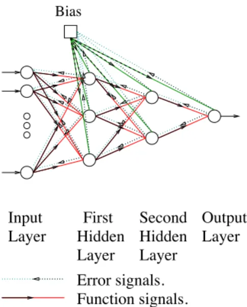
The most popular NN model is the multi-layer perceptron (MLP) since the formalization of the backpropagation (BP) leaning algorithm in the early 1980s. The basic design of an MLP is shown in Figure 1.
The input signal of an MLP (or feature vector) is propagated through the network (neuron by neuron), and transformed during its passage by the combination of the synaptic weights and mathematical properties of the neurons, until on the final layer an output signal is generated. In the example shown in Figure 1 the network is defined as being fully connected, each neuron (or node) being connected to each other neuron in the layers directly preceding and proceeding it, and having aI : 3 : 2 : 1 topological design. That is it hasIinput nodes, followed by twohidden layers, the first containing 3 nodes and the second 2 nodes, with a single output node. The two middle layers are referred to ashidden due the fact that the user does
Input Layer First Hidden Layer Second Hidden Layer Output Layer Error signals. Function signals. Bias
Fig. 1. Generic multi-layer perceptron, showing the forward flow of the input signal (function signal) and the backward flow of the error signal.
not commonly observe the inputs or outputs from these nodes (unlike the input layer where the feature vector is known and the output layer where the output is observed). The most common transfer function used in the MLP is the sigmoid function ϕ(). For the jth hidden node of a network with a vector ofzinputs its logistic form is defined as:
ϕ(z) = 1
1 + exp!−!Bj+"
|z|
i=1wi,jzi
## (1)
wherewi,j is theith input weight between nodej and the previous layer,
ziis the output of theith node in the layer preceding nodej andBj is the
weight of the bias input to thejth node. The bias is similar to the intercept term used in linear regression and has a fixed value for all patterns.
The adjustment of the synaptic weight parameter variables within an MLP are most commonly performed in asupervised learning manner using the fast backpropagation algorithm. Sequences of input and resultant out-puts are collected from an undefined functional processf(a)"→b. This set of patterns are then presented to the MLP in order for it to emulate the unknown function. Thekth input patterna(k) is fed through the network generating an output ˆb(k), an approximation of the desired output b (il-lustrated with the arrows pointing to the right in Figure 1). The difference
between the desired outputband the actual output ˆb(k) is calculated (usu-ally as the Euclidean distance between the vectors), and this error term, E, is then propagated back through the network, proportional to the par-tial derivative of the error at that node (illustrated with the dashed arrows pointing to the left in Figure 1). An in-depth discussion of the history and derivation of the backpropagation algorithm (and associated delta rule), through the calculus chain, can be found in Bishop5
and Haykin16 . Each pattern in turn is presented to the MLP, with its weights adjusted using the delta rule at each iteration. Only a fraction of the change demanded by the delta rule is usually applied to avoid rapid weight changes from one pattern to the next. This is known as the learning weight. A momentum term (ad-ditionally updating weights with a fraction of their previous update) is also commonly applied. The passing of an entire pattern set through the MLP is called a training epoch. MLPs are usually trained, epoch by epoch, until the observed average error of the function approximation reaches a plateau. The generalization ability of the approximated function is then assessed on another set of collected data which the NN has not been trained on.
In recent years there has been increasing interest in the use of evolution-ary computation methods for NN training.33
In these ENNs the adjustable parameters of an NN (weights and also sometimes nodes) are represented as a string of floating point and/or binary numbers, the most popular rep-resentation being the direct encoding form.33
Given a maximum size for a three layer feed-forward MLP ENN ofI input units (features), H hidden units in the hidden layer, and O output units, the vector length used to represent this network within an MOEA is of size:
(I+ 1)·H+ (H+ 1)·O+I+H (2) The first (I+ 1)·H + (H + 1)·O genes are floating point and store the weight parameters (plus biases) of the ENN, the next I+H are bit represented genes, whose value (0 or 1) denotes the presence of a unit or otherwise (in the hidden layer and input layer). Thesedecision vectors are manipulated over time using the tools of evolutionary computation (usually evolution strategies (ESs) or genetic algorithms (GAs)). At each time step (known as ageneration) the ENNs represented by the new decision vectors are evaluated on the training data, and selection for parameter adjustment in the next generation is typically based on their relative error on this data. The popularity of these approaches to NN training is that they are not susceptible to trapping in local minima that gradient descent based learning
algorithms are, and in addition, can use quite complex problem specific error functions which may be difficult to propagate using derivatives.
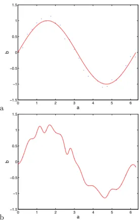
Because of the high function complexity that NNs can emulate, there is always a risk that the NN will simply map the input and output vectors directly without recourse to creating an internal representation of their generation process. An illustration of this is shown in Figure 2.
a 0 1 2 3 4 5 6 −1.5 −1 −0.5 0 0.5 1 1.5 a b b 0 1 2 3 4 5 6 −1.5 −1 −0.5 0 0.5 1 1.5 a b
Fig. 2. Overfitting illustration. Explanatory variableaand dependent variablebwith noise.Top: generating function.Bottom: overfitted signal.
In the illustration the model approximator is too complex, and therefore fits exactly to the noisy data points instead of modelling the smoother generating process.
3. Optimal model complexity
Procedures to prevent the over-fitting of NNs can be categorized as falling into two broad camps. The first group of methods take the approach that the model used may be over specified (have more complexity than is needed to model the problem), but by judicious use of more that one data set in the training process the risk of over fitting can be minimized. The type most frequently used is the so called ‘early stopping’ method, where a an additionalvalidation data set is used in the training process,25
other more advanced methods based on bootstrapping27
are also in use. The second group of methods tackles over-fitting with conscious attempts to restrict the complexity of the NN during its training process, sometimes in conjunction with early stopping methods.
3.1. Early stopping
There are a number of different approaches to early stopping.25
The tradi-tional approach is to train a network and monitor its generalization error on a validation set and stop training when the error on this set is seen to rise. The general problem with this approach is that the generalization curve may exhibit a number of local minima, so the early stopping may in fact be too ‘early’. In order to overcome this the NN is trained as normal, without stopping until the training error reaches a plateau, at the same time however the generalization error on a validation set is checked - and the network parameters when this is lowest recorded and used.
3.2. Weight decay regularization and summed penalty terms
One of the most common approaches to prevent over-fitting through com-plexity minimization is that of weight decay regularization. This approach attempts to inhibit the complexity of a particular model by restricting the size of its weights, as it is known that larger weights values are needed to model functions with a greater degree of curvature (and there-fore complexity).5
In its standard form the sum of the squares of the NN weights are used as a penalty term within the error function, such that
Enew=E+βΘ (3)
whereE is the default error function (commonly Euclidean error),Θis the sum of squares of the NN weights,β is a weighting term and Enew is the
Other approaches have been developed by researchers in the ENN field use slightly different summed penalty terms in NN training, for example Liu and Yao22
include a penalty for the size of the network in their composite error function.
3.3. Node and weight addition/deletion
Node pruning/addition techniques ignore the complexity through the weight value approach of weight decay regularization and some of the other complexity penalty term approaches, and instead couch the complexity of a NN in terms solely of the number of transformation nodes. The sim-plest methodology of this approach is exhaustive search, training many different NNs with different numbers of hidden units and comparing their performance against each other. The computation cost of this approach is obviously prohibitive, however it can be constrained to a certain degree by simply adding an additional node to a previously trained NN, using the weights of the previous network as a starting point. This method is described as a growing algorithm approach,5
cascade correlation being an-other.
In Kameyama and Kosugi17
the opposite approach is taken, with a large NN initially specified, followed by the selective pruning of NN units. Le-Cunet al.21
take a different approach of pruning, again citing that the best generalization is obtained by trading off the training error and network complexity, their method called optimal brain damage (OBD) focuses on removing NN weights. The basic idea is to choose a reasonable network architecture, train the network until a reasonable solution is obtained us-ing gradient descent methods and compute the second derivative for each parameter (NN weight). The parameters are then sorted by this saliency, and those parameters with low saliency are deleted. Ragg and Gutjahr26 in contrast use mutual information in their routine for topology determi-nation.
3.4. Problems with these methods
Network growing and pruning methods are usually characterized as being slow to converge, with long training time and, for those that use of gra-dient descent training techniques, susceptible to becoming stuck in local minima.3
The main criticism directed at weight decay regularization and other penalty term approaches to training, is the problem of how to spec-ify the weighting terms needed by these methods. Just as it is difficult to
ascertain the correct model complexity for a modela priori, so the correct degree of penalization to include in these adjusted error values is difficult to know beforehand. In addition the weighted sum approach is only able to get all points from a Pareto front when it is convex.7
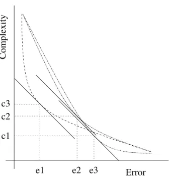
A demonstration of the problem of composite error weight specification is illustrated below in Figure 3.
Complexity
c1
c2
c3
Error
e1
e2 e3
Fig. 3. Illustration of the problems inherent in using composite error functions to de-termine an operating point.
Figure 3 shows three different fronts describing the trade-off between accuracy and complexity. Each with a line tangential to them at the point where the values are equal (equivalent toβ=1 in Equation 3). As can be seen in the illustration, depending upon the actual interaction of complex-ity and accuracy exhibited by the process, as described by the curves, three very different models will be returned by using this composite error weight-ing. One with high error, low complexity (e1, c3), one with intermediate complexity and error (e2, c2) and a third with low accuracy and low er-ror (e3, c1). Again, it must be noted that these results are dependent on the front shape, which is unknowna priori, but which must be implicitly
guessed at if the composite error approach is used. Of course it is feasible to run the composite error algorithm a number of times to discover the shape of the front, however the algorithm will need to be run as many times as the number of points desired, which is very time consuming, and even then non-convex portions of the front will remain undiscovered.
4. Using evolutionary algorithms to discover the complexity/accuracy trade-off
As discussed in Section 3, until recently researchers interested in constrain-ing the complexity of their models had to assign one or more variables, whose value was known to greatly affect the end model, but whose selec-tion was difficult, if not impossible, to assign without knowing how the model complexity and accuracy interacts for the specific problem. Instead of trying to simultaneously optimize these separate objectives by combin-ing complexity and accuracy into a scombin-ingle error value, which is shown to be problematic, they can be optimized as two separate objectives, through the use of EMOO techniques. By using this methodology a set of ENNs can be produced showing the realized complexity/accuracy trade-offfor each problem.
Before discussing this approach further however, the concept of Pareto optimality needs to be briefly described.
4.1. Pareto optimality
Most recent work in EMOO is formulated in terms of non-dominance and Pareto optimality.
The multi-objective optimization problem seeks to simultaneously ex-tremizeD objectives:
yi=fi(x), i= 1, . . . , D (4)
where each objective depends upon a vector x of P parameters or deci-sion variables, in the case of this chapter, ENN weights and nodes. The parameters may also be subject to theJ constraints:
ej(x)≥0, j= 1, . . . J. (5)
Without loss of generality it is assumed that the objectives are to be minimized, so that the multi-objective optimization problem may be ex-pressed as:
subject toe(x) = (e1(x), . . . , eJ(x))≥0 (7)
wherex= (x1, . . . , xP) andy= (y1, . . . , yD).
When faced with only a single objective an optimal solution is one which minimizes the objective given the model constraints. However, when there is more than one objective to be minimized solutions may exist for which performance on one objective cannot be improved without sacrificing per-formance on at least one other. Such solutions are said to be Pareto opti-mal30
after the 19th century Engineer, Economist and Sociologist Vilfredo Pareto, whose work on the distribution of wealth led to the development of these trade-offsurfaces.24
The set of all Pareto optimal solutions are said to form the true Pareto front.
The notion ofdominancemay be used to make Pareto optimality clearer. A decision vectoruis said tostrictly dominate anotherv(denotedu≺v) iff
fi(u)≤fi(v) ∀i= 1, . . . , D ∧ ∃i fi(u)< fi(v) (8)
Less stringently,uweakly dominates v(denoted u*v) iff
fi(u)≤fi(v) ∀i= 1, . . . , D. (9)
A set of M decision vectors{Wi} is said to be a non-dominated set (an
estimated Pareto front) if no member of the set is dominated by any other member:
Wi+≺Wj ∀i, j= 1, . . . , M. (10)
4.2. Extent, resolution and density of estimated Pareto set
There are a number of requirements of estimated Pareto fronts that re-searchers strive for their algorithms to produce. These can be broadly de-scribed as high accuracy, representative extent, minimum resolution and equal density.
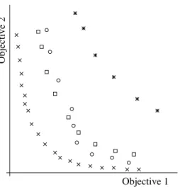
The first concept, accuracy, is simply that the estimated solutions should be as close as possible to the true Pareto front. As illustrated in Figure 4, the estimated front of AlgorithmA is clearly more accurate than that of AlgorithmB, however the comparison of A and C is more difficult to quantify, as some members of A dominate members of C, but also the reverse is true.
Ideally the Pareto solutions returned (or estimates of them) should lie across the entire surface of the true Pareto front, and not simply be con-cerned with a small subsection of it. Minimum resolution is a common
True Pareto Front
Estimated Pareto optimal individuals, algorithm A Estimated Pareto optimal individuals, algorithm B Estimated Pareto optimal individuals, algorithm C
Objective 1
Objective 2
Fig. 4. Illustration of the true Pareto front, and two estimates of it, estimate of algo-rithmAbeing clearly more accurate the B, but the comparison of AandC is not as easy to quantify.
requirement as in many applications the end user may wish the separation between potential solutions to be no bigger than a fixed value (of course, in discontinuous Pareto problems this requirement is not entirely realistic). Much emphasis has been placed by researchers on the non-dominated solutions returned by the search algorithm being equally distributed (of even density),9
however it is arguable that this should only be of concern if the generating process results in evenly distributed solutions. In an actual application it may well be the case that the generating process produces an unbalanced Pareto front, this information itself may be very pertinent to the decision maker – by forcing multi-objective evolutionary algorithms (MOEAs) to misrepresent this fact by penalizing any representation than equal density they may well have negative repercussions for the final user of the information.
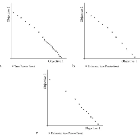
An illustration of this is provided in Figure 5. Figure 5a shows the true Pareto front, with Figures 5b and 5c illustrating the returned sets of two MOEAs, one which focuses on equal density and one that does not, Figure 5b gives no indication to the end user of the density of solutions to the
a
Objective 1
Objective 2
True Pareto Front b
Objective 1
Objective 2
Estimated true Pareto front
c
Objective 1
Objective 2
Estimated true Pareto Front
Fig. 5. Comparing the density of estimated Pareto fronts. Illustration of an underlying true Pareto front (a), and its approximation using an MOEA that is designed to return equal density along the front (b) and one that does not (c).
lower left of the front.
4.3. The use of EMOO
Abbass2,3
and Abbass and Sarker1
have recently applied EMOO techniques to trading offthe number of hidden units with respect to the accuracy of the NN, where each point on the Pareto frontier is therefore represented by an ENN with a different number of hidden units to any other set member. A description of their memetic Pareto artificial neural network (MPANN) model can be found in Algorithm 1.
The algorithm presented by Abbass is sufficient when concerned with NN complexity defined as the number of transfer units, but is insufficient when concerned with complexity defined as the number of weights or the
Algorithm 1The memetic Pareto artificial neural network algorithm.1,2,3 M, Size of initial random population of solutions.
N, Maximum number of EA generations.
E, Maximum number of backpropagation epochs.
1: Generate random NN population,S, of size M, such that each parameter (weight) of the NN, xi ∼N(0,1), and the binary part
of the decision vector is either initialized at one or∼U(0,1). 2: Initialize generation countert:= 0.
3: whilet < N
4: Find set of solutions withinS which are dominated,S,$ S:=S\S.$
5: if|S|<3
6: Insert members fromS$until|S|= 3.
7: end if
8: Randomly mark 20% of training data as validation data. 9: while|S|< M
10: Select random representatives fromS;x,yand z
11: xnew:=crossover(x,y,z)
12: xnew:=mutate(xnew)
13: xnew:=backpropagation(xnew, E)
14: ifxnew≺x 15: S:=S+xnew 16: end if 17: end while 18: t:=t+ 1 19: end while 20: end
sum of the squared weight values. This is because the algorithm internalises the estimated Pareto frontF within the search population, and needs the maximum size of the Pareto front to be less than that of the search pop-ulation. This can be seen at line 4 of Algorithm 1, where the dominated members of the search populationSare removed. If none of the search pop-ulation members are dominated (it is a mutually non-dominating set) then no further search will be promoted (line 9) and the Algorithm will simply do nothing until the maximum number of generations is reached. As the second objective in MPANN1,2,3
is discrete, with a maximum limit ofHmax
empirical applications1,2,3
the maximum number of hidden units was 10 and the search population size 50, this problem was not encountered, how-ever Algorithm 1 cannot be easily applied to situations where the second objective is to minimize the number of weights, as the maximum size ofF (for a single layer MLP) would beHmax×I+Hmax+Hmax+ 1 and the
search population would therefore need to be significantly greater than this. In the case of sum of squared weights then there is essentially no limit on the size of the Pareto set, and therefore no search population in Algorithm 1 would be large enough.
The method of search population update1,2,3
is essentially a variant of the conservative replacement scheme described by Hanne15
, where an in-dividual in the search population is only replaced if it is dominated by a perturbed copy of itself. In this chapter a more generally applicable algo-rithm will be described for the multi-objective evolution of NNs, with the emphasis placed on ease of encoding, for the trade-off of complexity and accuracy
4.4. A general model
Perhaps the simplest EA in common use is the ES, where the parameters are perturbed to adjust their value from one generation to the next. Its popularity is probably derived in part from its ease of encoding and use, however it has also formed the base of a number of successful algorithms in the MOEA domain, not least the Pareto archived evolutionary strategy (PAES) of Knowles and Corne.18,19
Due to its simplicity and previous suc-cess it is also used as the base of Algorithm 2, which is used here to search for the complexity/accuracy trade-offfront.
4.4.1. mutate()
In ES, the weight space of a network is perturbed by set of values drawn at each generation from a known distribution, as shown in Equation 11.
xi=xi+γ·Θ (11)
wherexiis theithdecision parameter of a vector,Θis a random value drawn
from some (pre-determined) distribution andγis some multiplier. A (µ,λ )-ES process is one in whichµdecision vectors are available at the start of a generation (called parents), which are then perturbed to generateλvariants of themselves (called children or offspring). This set of λ children is then truncated to provide theµ parents of the following iteration (generation).
Algorithm 2 The ES based MO training algorithm for complex-ity/accuracy trade-offdiscovery.
M, Size of initial random population of solutions. N, Maximum number of EA generations.
pmut, Probability of weight perturbation.
pw, Probability of weight removal.
pu, Probability of unit removal
E, Maximum number of backpropagation epochs. 1: Initialise NN individual z.
2: z:=backpropagation(z, E)
3: Generate random NN population, S, of sizeM, such that each parameter (weight) of the NN, xi ∼N(zi,1), and the binary part
of the decision vector is either initialised at one or ∼U(0,1). 4: F0=∅. UpdateF0 with the non-dominated solutions fromS∪z 5: Initialise generation countert:= 0.
6: whilet < N
7: Create copy of search population,S$:=S
8: fori= 1 :M
9: S$i:=mutate(S$i, pmut)
10: S$i:=weightadjust(S$i, pw)
11: S$i:=unitadjust(S$i, pu)
12: end for
13: UpdateF0 with the non-dominated solutions fromS$ 14: fori= 1 :M 15: ifS$i≺Si 16: Si:=S$i 17: else ifS$i⊀Si 18: if 0.5>U(0,1) 19: Si:=S$i 20: end if 21: end if 22: end for 23: S:=replace(S, F,M 5) 24: t:=t+ 1 25: end while 27: end
The process of selection for which children should form the set of parents in the next iteration is usually dependent on their evaluated fitness (the fitter being more probable to ‘survive’). A (µ+λ)-ES process denotes one where the parents compete with the children in the selection process for the next generation parent set, which is the method used in Algorithm 2. Recent work in the field of EAs has shown that the use of heavier tailed distributions can speed up algorithm performance34
and as such in this chapter Θ is a Laplacian distribution with width parameter 1, and γ = 0.1. In Algorithm 2mutate(x, pmut) perturbs the weight parameters of the
decision vectorxwith a probability ofpmut.
4.4.2. weightadjust()
In order for partially connected ENNs to lie within the search space of the algorithm, theweightadjust() method is used (line 10 of Algorithm 2). weightadjust(x, pw) acts upon the weight parameters ofx, setting them to
0 with a probability ofpw(effectively removing them).
4.4.3. unitadjust()
Topography and input feature selection is implemented within the model by bit mutation of the section of the decision vector representing the network architecture. This is facilitated by first determining a super-set of input features and maximum hidden layer sizes. Once this is determined, any individual has a fixed maximum representation capability. Manipulation of structure is stochastic. By randomly bit flipping members of the first I genes of the binary section of the decision vector the set of input features used by the network is adjusted, and flipping the followingH genes affects the hidden layer.
4.4.4. The elite archive
In addition to the search populationS Algorithm 2 also maintains an elite archiveFof the non-dominated solutions (ENNs) found so far in the search process. No truncation is used on this set as the process can lead to some negative repercussions; it can cause some members ofF to be dominated by members ofF from an earlier generation (empirical proof of this can be found in Fieldsend11
and theoretical justification in Hanne15
). It also means that the final front discovered should be distributed in a way more indicative of the underlying process, as discussed in Section 4.2. Time concerns can be
addressed by the efficient use of data structures,10,11,12,23
however if growth is significant then some form of truncation may be worth considering.20 4.4.5. replace()
In order to promote additional search pressure on S in Algorithm 2, the replace(S, F,M
5) function updates S by randomly replacing a fifth (M/5) of its decision vectors with copies of individuals fromF. These copies are selected using partitioned quasi-random selection (PQRS),12
which ensures that a good spread of solutions is selected from the estimated Pareto front.
4.5. Implementation and generalization
A number of recent approaches to training ENNs when simultaneously ad-justing topology have done so using a hybrid approach, where training with EA methods and gradient descent techniques has been inter-levered.1,2,3,22 Justification for this approach has been made for the very sensible reason of computational efficiency - by using a hybrid learning approach as opposed to a purely EA training methodology the training time is typically reduced. However this is not to say that hybrid training does not create problems of its own, if the problem at hand demands a ‘hand crafted’ error func-tion, like many in financial forecasting applications,4,11,13,28,32
they may be difficult to propagate through gradient descent learning methods. Recent work has highlighted that the most profitable model is not necessarily the one that minimizes forecast Euclidean error.11,13
. As such the method de-scribed in this chapter uses traditional gradient descent methods to seed to search process, line 2 of Algorithm 2, but thereafter is exclusively EA driven, meaning it is easily applicable to the widest range of time series forecast problems with minimal modification requirements.
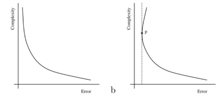
Algorithm 2 deals solely with fitting the ENNs to a set of training data, which then leads us to the question of how to minimize generalization error with this information? The approach advocated in this chapter is disarm-ingly simple. Instead of convoluted training and validation during the train-ing process, validation error/complexity is compared to the Pareto traintrain-ing error/complexity after training, and a suitable operating ENN chosen using this comparison. An illustration of this is provided in Figure 6.
The curve on Figure 6a illustrates the complexity/accuracy trade-off curve discovered on a set of training data, and Figure 6b illustrates the same ENNs evaluated on some validation data. This curve can be seen as being non-Pareto, as it curves back on itself at high-complexity, showing
a Complexity Error b Complexity Error p
Fig. 6. Illustration of the complexity/error trade-offfront. Left: Training data Pareto front, Right: the same ENNs evaluated on validation data, from point ‘p’ onwards the ENNs are overfitted and should not be used.
that those networks have been overfitted. The practitioner should there-fore operate with ENN at point ‘p’ if they wish to minimize generalization error, or at a complexity below that if they have constraints on the dis-tributed complexity of their model (if for instance they are content with a lower accuracy if they can reduce the number of transfer units/weights in the network). The actual generalization error can then be assessed on some additional unseen test data to reassure the choice of complexity. This ap-proach has an advantage over the common early stopping method described earlier, in that it doesn’t have the potential to be trapped in local minima, and it promotes search in areas which are not confined to the gradient descent weight trajectory.
5. Empirical validation
The methodology introduced in the previous section will now be validated. Two different measures of complexity will be modelled – that of the sum of the squared weights, and the number of weights used. Results from choosing the model at point ‘p’ will be compared to the traditional approach of early stopping on time series problems with various degrees of noise, and example fronts produced to support the general methodology.
5.1. Data
The data used will be of a physical process, the oscillation of a laser,a where an underlying function is thought to drive the observations, but where there
a
The time series data, with full descriptions, can be found at http://www-psych.stanford.edu/˜andreas/Time-Series/SantaFe.html .
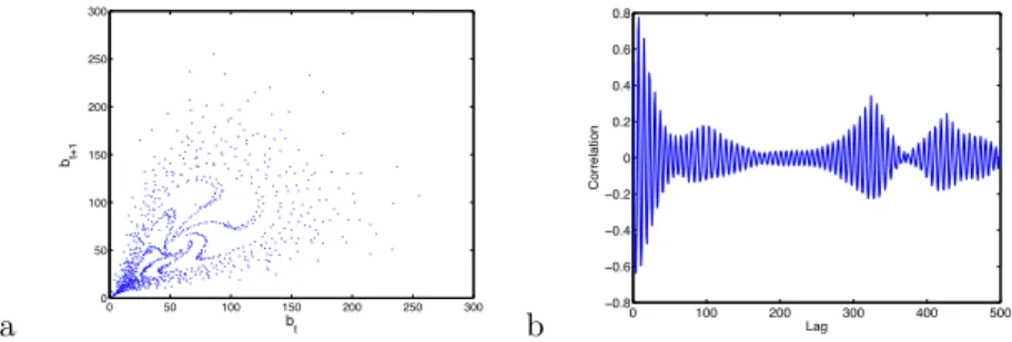
is also a degree of measurement noise. Additional noise will be added to these processes in order to promote lower complexity representations and penalize high complexity representations. A plot of the training data is shown in Figure 7, Figure 8a shows the scatter plot of the time series versus its first lag, and Figure 8b shows the correlation coefficient values for different lags of this data.
0 100 200 300 400 500 600 700 800 900 1000 0 50 100 150 200 250 300 Time Value
Fig. 7. Laser oscillation time series.
On inspection of the correlation coefficient values, 40 lags were decided to be used to model the process, resulting in 960 input/output pairings. This data was then randomly partitioned into an ENN training set of 640 samples and validation set of 220 samples. The unseen test set consisted of 9053 input/output pairings. a 0 50 100 150 200 250 300 0 50 100 150 200 250 300 bt bt+1 b −0.80 100 200 300 400 500 −0.6 −0.4 −0.2 0 0.2 0.4 0.6 0.8 Lag Correlation
Fig. 8. Laser oscillation time series. Left: Scatter plot of current value against previous value. Right: Correlation coefficient values for different lags of time series.
Ten different variants of the series where subsequently made with differ-ent degrees of additional noise, drawn from a Gaussian, to mimic differdiffer-ent
levels of measurement corruption, making a total of eleven time series, each with a different propensity to overfitting.
5.2. Model parameters
MOEA training was applied through the process described in Algorithm 2, with the following parameters:Hmax= 10,γ= 0.1,pmut= 0.2,pw= 0.02,
pu = 0.02, N = 5000,E = 5000 and |S| = 100. In addition, a NN was
trained for each of the time series using the more advanced early stopping method described in subsection 3.1, for 20000 epochs. The leaning rate for all algorithms using backpropagation was 0.05, with a momentum term of 0.5. In addition the MOEA with the minimizing sum of squared weights objective updatedF during the initial training of the seed neural network, this was found to improve training as it gave a good first estimate of the trade-offfront.
6. Results
Figure 9 is an indicative plot of the realized fronts created by the set of op-timal ENNsF evaluated on the training, validation and test sets. Although the set is mutually non-dominating on the training data, the validation and test data sets both exhibit the folding-back predicted in the previous section, indicating the ENN to select if the user is solely concerned with minimising generalization error. The point at which this fold back occurs is observed to lower as the amount of noise increases (see Table 1).
Figure 10 on the other hand shows the evaluation of ENNs training with the second objective of number of weights minimization. The size of F at the end of this process is substantially smaller than that of squared sum of weights minimization (averaging around 100 as opposed to over 10000), however this form of training can be viewed as more useful to the practitioner who is concerned with the trade-offof accuracy versus actual NN size, as shows that the NN can be drastically reduced with only a marginal increase in error, if they wish to distribute a far simpler model.
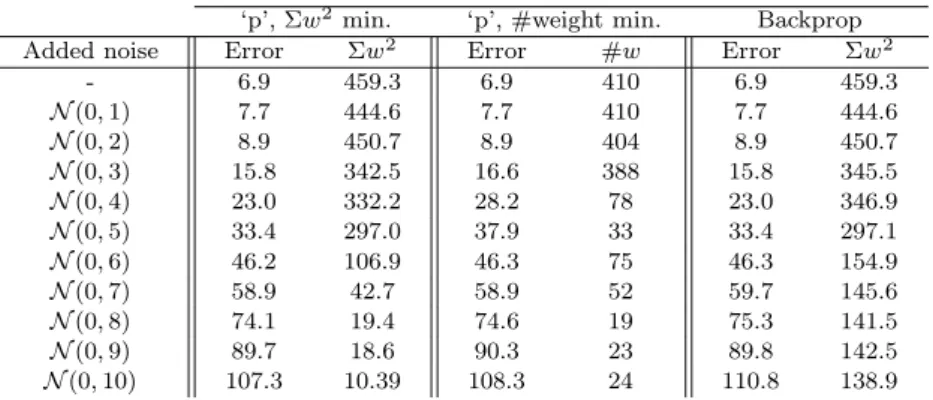
Table 1 gives the error and ‘complexity’ of the different models selected at ‘p’ by the MOEAs with the different complexity objectives for the 11 data sets, along with that of a NN trained in the traditional early stopping fashion. The error rates can be seen to be equivalent, with the MOEAs seeming to perform slightly better as the amount of noise increases. The MOEA models minimizing sum of the squared weights can also be seen to have much lower weight values compared to the early stopping approach as
10 20 30 40 50 60 70 80 90 0 100 200 300 400 500 600 Error Training evaluation Validation evaluation Testing evaluation
Fig. 9. Training, validation and test set fronts for the error and Σw2
minimization training process, with additional noiseN(0,4). The phenomena of the validation and
test set fronts folding back on itself can be clearly seen.
0 10 20 30 40 50 60 70 80 90 0 50 100 150 200 250 300 350 400 450 Error Number of weights Training evaluation Validation evaluation Testing evaluation
Fig. 10. Training, validation and test set fronts for the error and #w minimization training process, without additional noise. The user now gains the information that the number of active weights (connectivity) of the NN can be drastically reduced with only a marginal increase in error, if they wish to distribute a far simpler model.
the noise increases. 7. Discussion
EMOO approaches to NN training have already proved useful in providing trade-offfronts between competing error objectives in financial time series
Table 1. Results of single ENN model selected at point ‘p’ on validation front, and an early stopping backpropagation NN.
‘p’,Σw2
min. ‘p’, #weight min. Backprop Added noise Error Σw2
Error #w Error Σw2 - 6.9 459.3 6.9 410 6.9 459.3 N(0,1) 7.7 444.6 7.7 410 7.7 444.6 N(0,2) 8.9 450.7 8.9 404 8.9 450.7 N(0,3) 15.8 342.5 16.6 388 15.8 345.5 N(0,4) 23.0 332.2 28.2 78 23.0 346.9 N(0,5) 33.4 297.0 37.9 33 33.4 297.1 N(0,6) 46.2 106.9 46.3 75 46.3 154.9 N(0,7) 58.9 42.7 58.9 52 59.7 145.6 N(0,8) 74.1 19.4 74.6 19 75.3 141.5 N(0,9) 89.7 18.6 90.3 23 89.8 142.5 N(0,10) 107.3 10.39 108.3 24 110.8 138.9 forecasting,11,13
and a methodology already exists for learning the trade-off front between NN accuracy and the number of hidden units.1,2,3
The methodology described in this chapter takes this further and presents a pro-cess for encapsulating other definitions of NN complexity within a MOEA training process. These have been shown to be equivalent or better than the popular early stopping approach to NN training on a physical time se-ries process with many different degrees of noise, and therefore over-fitting propensity, for the selection of a single ‘best’ NN in terms of generaliza-tion error. However more importantly, by using the assessment of a set of estimated Pareto optimal ENNs on validation data, the non-dominated ENNs can give the user a good representation of the complexity/accuracy trade-off of their problem, such that NNs with very low complexity may feasibly be used. In the example series used in this paper the cost in terms of realized error of this approach was surprising low.
Acknowledgements
Jonathan Fieldsend gratefully acknowledges support from the EPRSC grant number GR/R24357/01 during the writing of this chapter.
References
1. H. Abbass and R. Sarker. Simultaneous evolution of architectures and con-nection weights in anns. In Artificial Neural Networks and Expert Systems Conference, pages 16–21, Dunedin, New Zealand, 2001.
2. H.A. Abbass. A Memetic Pareto Evolutionary Approach to Artificial Neu-ral Networks. InThe Australian Joint Conference on Artificial Intelligence, pages 1–12. Springer, 2001.
3. H.A. Abbass. An Evolutionary Artificial Neural Networks Approach for Breast Cancer Diagnosis. Artificial Intelligence in Medicine, 25(3):265–281, 2002.
4. J.S. Armstrong and F. Collopy. Error measures for generalizing about fore-casting methods: Empirical comparisons. International Journal of Forecast-ing, 8(1):69–80, 1992.
5. C.M. Bishop. Neural Networks for Pattern Recognition. Oxford University Press, 1998.
6. C.A.C Coello. A Comprehensive Survey of Evolutionary-Based Multiobjec-tive Optimization Techniques.Knowledge and Information Systems. An In-ternational Journal, 1(3):269–308, 1999.
7. I. Das and J.Dennis. A closer look at drawbacks of minimizing weighted sums of objectives for pareto set generation in multicriteria optimization problems. Structural Optimization, 14(1):63–69, 1997.
8. K. Deb. Multi-objective genetic algorithms: Problem difficulties and con-struction of test problems. Evolutionary Computation, 7(3):205–230, 1999. 9. K. Deb, L. Thiele, M. Laumanns, and E. Zitzler. Scalable Multi-Objective
Optimization Test Problems. In Congress on Evolutionary Computation (CEC’2002), volume 1, pages 825–830, Piscataway, New Jersey, May 2002. IEEE Service Center.
10. R.M. Everson, J.E. Fieldsend, and S. Singh. Full Elite Sets for Multi-Objective Optimisation. In I.C. Parmee, editor,Adaptive Computing in De-sign and Manufacture V, pages 343–354. Springer, 2002.
11. J.E. Fieldsend.Novel Algorithms for Multi-Objective Search and their appli-cation in Multi-Objective Evolutionary Neural Network Training. PhD thesis, Department of Computer Science, University of Exeter, June 2003.
12. J.E. Fieldsend, R.M. Everson, and S. Singh. Using Unconstrained Elite Archives for Multi-Objective Optimisation. IEEE Transactions on Evolu-tionary Computation, 7(3):305–323, 2003.
13. J.E. Fieldsend and S. Singh. Pareto Multi-Objective Non-Linear Regression Modelling to Aid CAPM Analogous Forecasting. InProceedings of the 2002 IEEE International Joint Conference on Neural Networks, pages 388–393, Hawaii, May 12-17, 2002. IEEE Press.
14. C.M. Fonseca and P.J. Fleming. An Overview of Evolutionary Algorithms in Multiobjective Optimization.Evolutionary Computation, 3(1):1–16, 1995. 15. T. Hanne. On the convergence of multiobjective evolutionary algorithms.
European Journal of Operational Research, 117:553–564, 1999.
16. S. Haykin.Neural Networks A Comprehensive Foundation. Prentice Hall, 2 edition, 1999.
17. K. Kameyama and Y. Kosugi. Automatic fusion and splitting of artificial neural elements in optimizing the network size. In Proceedings of the In-ternational Conference on Systems, Man and Cybernetics, volume 3, pages 1633–1638, 1991.
18. J. Knowles and D. Corne. The pareto archived evolution strategy: A new baseline algorithm for pareto multiobjective optimisation. InProceedings of the 1999 Congress on Evolutionary Computation, pages 98–105, Piscataway,
NJ, 1999. IEEE Service Center.
19. J.D. Knowles and D. Corne. Approximating the Nondominated Front Us-ing the Pareto Archived Evolution Strategy. Evolutionary Computation, 8(2):149–172, 2000.
20. J.D. Knowles and D. Corne. Properties of an Adaptive Archiving Algo-rithm for Storing Nondominated Vectors.IEEE Transactions on Evolution-ary Computation, 7(2):100–116, 2003.
21. Y. LeCun, J. Denker, S. Solla, R. E. Howard, and L. D. Jackel. Optimal brain damage. In D. S. Touretzky, editor,Advances in Neural Information Process-ing Systems II, pages 598–605, San Mateo, CA, 1990. Morgan Kauffman. 22. Y. Liu and X. Yao. Towards designing neural network ensembles by
evolu-tion.Lecture Notes in Computer Science, 1498:623–632, 1998.
23. S. Mostaghim, J. Teich, and A. Tyagi. Comparison of Data Structures for Storing Pareto-sets in MOEAs. In Congess on Evolutionary Computation (CEC’2002), volume 1, pages 843–848, Piscataway, New Jersey, May 2002. IEEE Press.
24. V. Pareto.Manuel D’ ´Economie Politique. Marcel Giard, Paris, 2nd edition, 1927.
25. L. Prechelt. Automatic early stopping using cross validation: quantifying the criteria.Neural Networks, 11(4):761–767, 1998.
26. T. Ragg and S. Gutjahr. Automatic determination of optimal network topolo-gies based on information theory and evolution. In IEEE Proceedings of the 23rd EUROMICRO Conference, pages 549–555. IEEE Compter Society Press, 1997.
27. Y. Raviv and N. Intrator. Bootstrapping with noise: An effective regulariza-tion technique.Connection Science, 8:356–372, 1996.
28. E. Saad, D. Prokhorov, and D. Wunsch. Comparative Study of Stock Trend Prediction Using Time Delay, Recurrent and Probabilistic Neural Networks. IEEE Transactions on Neural Networks, 9(6):1456–1470, 1998.
29. J. Utans and J. Moody. Selecting neural network architectures via the predic-tion risk: applicapredic-tion to corporate bond rating predicpredic-tion. InProc. of the First Int. Conf on AI Applications on Wall Street, pages 35–41, Los Alamos,CA, 1991. IEEE Computer Society Press.
30. D. Van Veldhuizen and G. Lamont. Multiobjective Evolutionary Algorithms: Analyzing the State-of-the-Art. Evolutionary Computation, 8(2):125–147, 2000.
31. D. Wolpert. On bias plus variance. Neural Computation, 9(6):1211–1243, 1997.
32. J. Yao and C.L. Tan. Time Dependant Directional Profit Model for Fi-nancial Time Series Forecasting. In Proceedings of IJCNN 2000, Como IEEE/INNS/ENNS, volume 5, pages 291–296, 2000.
33. X. Yao. Evolving Artificial Neural Networks. Proceedings of the IEEE, 87(9):1423–1447, 1999.
34. X. Yao, Y. Liu, and G. Lin. Evolutionary Programming Made Faster.IEEE Transactions on Evolutionary Computation, 3(2):82–102, 1999.