Multimodal learning from visual and
remotely sensed data
Dushyant Rao, BE (Hons 1) BSc, MSc
A thesis submitted in fulfillment of the requirements of the degree of
Doctor of Philosophy
Australian Centre for Field Robotics
School of Aerospace, Mechanical and Mechatronic Engineering The University of Sydney
Declaration
I hereby declare that this submission is my own work and that, to the best of my knowledge and belief, it contains no material previously published or written by another person nor material which to a substantial extent has been accepted for the award of any other degree or diploma of the University or other institute of higher learning, except where due acknowledgement has been made in the text.
Dushyant Rao, BE (Hons 1) BSc, MSc
Abstract
Dushyant Rao, BE (Hons 1) BSc, MSc Doctor of Philosophy
The University of Sydney July 2016
Multimodal learning from visual and
remotely sensed data
Autonomous vehicles are often deployed to perform exploration and monitoring mis-sions in unseen environments. In such applications, there is often a compromise between the information richness and the acquisition cost of different sensor modali-ties. Visual data is usually very information-rich, but requires in-situ acquisition with the robot. In contrast, remotely sensed data has a larger range and footprint, and may be available prior to a mission. In order to effectively and efficiently explore and monitor the environment, it is critical to make use of all of the sensory information available to the robot.
One important application is the use of an Autonomous Underwater Vehicle (AUV) to survey the ocean floor. AUVs can take high resolution in-situ photographs of the sea floor, which can be used to classify different regions into various habitat classes that summarise the observed physical and biological properties. This is known as
benthic habitat mapping. However, since AUVs can only image a tiny fraction of the ocean floor, habitat mapping is usually performed with remotely sensed bathymetry (ocean depth) data, obtained from shipborne multibeam sonar.
With the recent surge in unsupervised feature learning and deep learning techniques, a number of previous techniques have investigated the concept of multimodal learning: capturing the relationship between different sensor modalities in order to perform classification and other inference tasks. This thesis proposes related techniques for visual and remotely sensed data, applied to the task of autonomous exploration and
monitoring with an AUV. Doing so enables more accurate classification of the benthic environment, and also assists autonomous survey planning.
The first contribution of this thesis is to apply unsupervised feature learning tech-niques to marine data. The proposed techtech-niques are used to extract features from image and bathymetric data separately, and the performance is compared to that with more traditionally used features for each sensor modality.
The second contribution is the development of a multimodal learning architecture that captures the relationship between the two modalities. The model is robust to missing modalities, which means it can extract better features for large-scale benthic habitat mapping, where only bathymetry is available. The model is used to perform classification with various combinations of modalities, demonstrating that multimodal learning provides a large performance improvement over the baseline case.
The third contribution is an extension of the standard learning architecture using a gated feature learning model, which enables the model to better capture the ‘one-to-many’ relationship between visual and bathymetric data. This opens up further inference capabilities, with the ability to predict visual features from bathymetric data, which allows image-based queries. Such queries are useful for AUV survey planning, especially when supervised labels are unavailable.
The final contribution is the novel derivation of a number of information-theoretic measures to aid survey planning. The proposed measures predict the utility of unob-served areas, in terms of the amount of expected additional visual information. As such, they are able to produce utility maps over a large region that can be used by the AUV to determine the most informative locations from a set of candidate missions. The models proposed in this thesis are validated through extensive experiments on real marine data. Furthermore, the introduced techniques have applications in various other areas within robotics. As such, this thesis concludes with a discussion on the broader implications of these contributions, and the future research directions that arise as a result of this work.
Acknowledgements
This thesis would not have been possible without the help and support of an enormous number of people.
First and foremost, I am eternally grateful to my supervisors, Stefan Williams and Oscar Pizarro, for providing support when I needed it, but allowing me the freedom to pursue my interests. You provided so many opportunities (very few people are priv-ileged enough to visit the Caribbean for research purposes), and made the daunting task of completing a PhD into an incredibly fun and rewarding experience.
To all my ACFR friends (you know who you are), thanks for keeping me sane and providing the perfect balance between academic discussions and distractions. I’ll truly miss our coffee breaks, despite the fact that I’m barely a coffee person - clearly there was another more important ingredient there!
To my family, thanks for keeping me grounded in reality and reminding me there’s a whole wide world out there. And in particular, to Shrutie, thanks for the love and support you have given me over the years, and for happily being the breadwinner in this family!
Contents
Declaration i
Abstract iii
Acknowledgements v
Contents vii
List of Figures xiii
List of Tables xv
List of Algorithms xvii
List of Authored Publications xix
Nomenclature xxi 1 Introduction 1 1.1 Motivation . . . 1 1.2 Problem statement . . . 3 1.3 Contributions . . . 4 1.4 Outline . . . 5
2 Background 7
2.1 Semantic classification and mapping . . . 7
2.2 Benthic habitat classification . . . 8
2.3 Unsupervised Feature Learning models . . . 10
2.3.1 Overview . . . 11
2.3.2 Autoencoders . . . 11
2.3.2.1 Regularisation and Sparsity . . . 13
2.3.3 Denoising Autoencoders . . . 14
2.3.4 Restricted Boltzmann Machines . . . 15
2.3.4.1 Training . . . 16
2.3.5 The connection between AEs and RBMs . . . 17
2.3.6 Other single layer learners . . . 19
2.4 Deep Learning models . . . 21
2.4.1 Feedforward Neural Networks . . . 21
2.4.2 Deep Belief Networks . . . 23
2.4.3 Convolutional Neural Networks . . . 25
2.4.3.1 Dropout . . . 26
2.4.4 Applications . . . 27
2.5 Multimodal learning . . . 28
2.6 Summary . . . 30
3 Learning features from marine data 31 3.1 Datasets . . . 32
3.1.1 Bathymetry . . . 32
3.1.2 Visual Images . . . 33
3.1.3 Co-located multimodal data . . . 34
3.1.4 Notation . . . 39
3.2 Classification problem setup . . . 40
Contents ix
3.3.1 Local bathymetry Bl . . . 41
3.3.2 DepthB0 . . . 42
3.3.3 Experiments . . . 43
3.3.3.1 Feature Learning . . . 44
3.3.3.2 Analysis of traditional bathymetric features . . . 45
3.3.3.3 Classification . . . 47
3.3.3.4 Habitat Mapping . . . 47
3.4 Visual Feature Learning . . . 52
3.4.1 Sparse Coding Spatial Pyramid Matching . . . 52
3.4.1.1 Dictionary Learning . . . 53
3.4.1.2 Sparse Encoding . . . 54
3.4.1.3 Spatial Pyramid Matching . . . 54
3.4.1.4 Additional Processing . . . 55
3.4.1.5 Discussion . . . 55
3.4.2 Convolutional Neural Networks . . . 56
3.4.3 Experiments . . . 58
3.4.3.1 Learned features . . . 58
3.4.3.2 Classification . . . 60
3.5 Summary . . . 62
4 Multimodal learning from visual and bathymetric features 63 4.1 Model description . . . 63
4.2 Inference . . . 65
4.2.1 Classification and habitat mapping . . . 65
4.2.2 Prediction and sampling . . . 66
4.3 Experiments . . . 67
4.3.1 Classification . . . 68
4.3.2 Precision and recall analysis . . . 70
4.3.3 Feature space analysis . . . 72
4.3.4 Habitat Mapping . . . 76
4.3.5 Generative Sampling . . . 76
5 Extending multimodal learning with gated models 81
5.1 Motivation . . . 82
5.2 Gated Boltzmann Machines and mixtures of RBMs . . . 83
5.3 Learning . . . 86 5.3.1 Cluster Heuristics . . . 86 5.3.1.1 Removing clusters . . . 87 5.3.1.2 Splitting clusters . . . 87 5.4 Inference . . . 88 5.4.1 Joint Sampling . . . 88
5.4.2 Conditional Sampling and Prediction . . . 88
5.4.3 Image-based queries . . . 90
5.4.4 Classification . . . 91
5.5 Experiments . . . 92
5.5.1 Toy Experiments . . . 92
5.5.2 Classification . . . 95
5.5.3 Precision and recall analysis . . . 95
5.5.4 Feature space analysis . . . 96
5.5.5 Habitat Mapping . . . 99
5.5.6 Clustering . . . 101
5.5.7 Visual prediction and image-based queries . . . 103
5.6 Summary . . . 104
6 Information-theoretic measures for AUV survey planning 107 6.1 Overview . . . 107
6.2 A primer on information theory . . . 108
6.2.1 Application to autonomous exploration . . . 110
6.3 Information-theoretic measures for survey planning . . . 113
6.3.1 Conditional mutual information . . . 113
Contents xi
6.4 Experiments . . . 117
6.4.1 Toy results . . . 117
6.4.2 Predictive utility mapping . . . 119
6.4.3 Survey selection . . . 121
6.5 Summary . . . 124
7 Conclusions 125 7.1 Contributions . . . 126
7.1.1 Feature learning from marine data . . . 126
7.1.2 Multimodal learning from visual and bathymetric data . . . . 126
7.1.3 Gated models for multimodal learning . . . 127
7.1.4 Information-theoretic measures for survey selection . . . 127
7.2 Future Work . . . 128
7.2.1 Multimodal learning for autonomous ground vehicles . . . 128
7.2.2 Incorporation of acoustic backscatter data and other modalities 129 7.2.3 Information-theoretic trajectory planning . . . 129
7.2.4 Improved training of gated models . . . 130
7.2.5 Experimental validation across multiple environments . . . 130
List of Figures
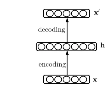
2.1 Graphical representation of an autoencoder . . . 12
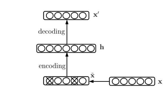
2.2 Graphical representation of a denoising autoencoder . . . 14
2.3 Graphical representation of a Restricted Boltzmann Machine. . . 16
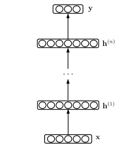
2.4 Graphical representation of a feedforward neural network. . . 22
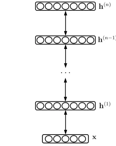
2.5 Graphical representation of a Deep Belief Network. . . 24
2.6 Examples of deep multimodal architectures used in previous work. . . 28
3.1 The gridded bathymetry data over the entire Southeastern Tasmania region . . . 33
3.2 The original label classes for the data, and the consolidated habitat classes. . . 35
3.3 Surveys performed in Southeastern Tasmania in 2008 (a) . . . 36
3.4 Surveys performed in Southeastern Tasmania in 2008 (b) . . . 37
3.5 An illustration showing how images from an AUV transect are matched to the corresponding bathymetry . . . 38
3.6 Examples of the matched multimodal data . . . 39
3.7 Examples of the features learned from bathymetry patches . . . 44
3.8 Habitat mapping results for the O’Hara Bluff region using the bathy-metric features . . . 49
3.9 Depth histograms for each habitat class . . . 51
3.10 Examples of the features learned from visual images . . . 59
4.1 The proposed model for multimodal learning . . . 64
4.3 The first four principal components for midlayer features . . . 74 4.4 The first four principal components for shared layer features . . . 75 4.5 Habitat mapping results for the O’Hara Bluff region using shared layer
features . . . 77 4.6 Bathymetric patch samples obtained from the learned data-generating
distribution, conditioned on an input image . . . 78 4.7 Depth samples obtained from the learned data-generating distribution,
conditioned on an input image . . . 79
5.1 Schematic showing the gated multimodal architecture . . . 83 5.2 Graphical representation of a gated mixture of RBMs . . . 84 5.3 Clustering and sampling results for the gated model on a toy dataset 93 5.4 Precision-recall curves for the gated multimodal model . . . 97 5.5 The first four principal components for gated shared layer features . . 98 5.6 Habitat mapping results for the O’Hara Bluff region using gated layer
features . . . 100 5.7 Examples of the clusters found by the gated model . . . 102 5.8 Image-based query results for images from different habitat classes . . 105
6.1 Venn diagram showing the conditional mutual information term and its dependence on the entropies of the individual modalities. . . 114 6.2 Analysis of information-theoretic metrics on a toy dataset . . . 118 6.3 Information-theoretic utility maps generated for the O’Hara Bluff region120 6.4 Predicted utility versus true utility for each dive in the SE Tasmania
List of Tables
3.1 Number of labels for each habitat class . . . 35 3.2 Spearman rank coefficient (ρ) when using learned features to predict
rugosity, slope, and aspect features . . . 46 3.3 Classification accuracy (%) of rugosity, slope, and aspect features . . 46 3.4 Classification accuracy of various bathymetric features . . . 48 3.5 The parameters for the convolutional neural network models applied
to visual classification . . . 57 3.6 Classification accuracy of visual features . . . 61
4.1 Classification accuracy for various input modalities using the multi-modal model . . . 69 4.2 Rugosity of bathymetric patch samples obtained from the learned
data-generating distribution, conditioned on an input image . . . 80
5.1 Classification accuracy for various input modalities using the gated multi-modality model . . . 96 5.2 A number of clustering performance metrics for the different input
modality scenarios. . . 103
List of Algorithms
2.1 Contrastive Divergence (CD-1) training for RBMs . . . 18
3.1 Orthogonal Matching Pursuit algorithm . . . 54
5.1 Contrastive Divergence (CD-1) training for a gated mixture of Restricted Boltzmann Machines . . . 87 5.2 Predicting visual features from bathymetry . . . 89
List of Authored Publications
D. Rao, M. De Deuge, N. Nourani-Vatani, B. Douillard, S. B. Williams, O. Pizarro.
Multimodal learning for autonomous underwater vehicles from visual and bathymetric data, inIEEE International Conference on Robotics and Automation, 2014, pp. 3819-25.
D. Rao, M. De Deuge, N. Nourani-Vatani, S. B. Williams, O. Pizarro. Multi-modality learning from visual and remotely sensed data, in IEEE/RSJ In-ternational Conference on Intelligent Robots and Systems, Workshop on Alternative Sensing and Robot Perception, 2015.
M. S. Bewley, N. Nourani-Vatani, D. Rao, O. Pizarro, S. B. Williams. Hierar-chical classification in AUV imagery, in Field and Service Robotics, 2015, pp. 3-16.
D. Rao, A. Bender, S. B. Williams, O. Pizarro. Multimodal information-theoretic measures for autonomous exploration, in IEEE International Conference on Robotics and Automation, 2016, pp. 4230-37.
D. Rao, M. De Deuge, N. Nourani-Vatani, S. B. Williams, O. Pizarro. Multimodal learning and inference from visual and remotely sensed data, inInternational Journal of Robotics Research, under review, 2016.
Nomenclature
Notation
a Visible bias vector or matrix b Hidden bias vector or matrix
E(·) Energy function
F(·) Free energy function
h Hidden units
i Index to an input variable
j Index to a hidden variable
k Index to a mixture indicator variable or label variable W Weights matrix or tensor
x Generic input variable or visible units x0 Input reconstruction
˜
x Corrupted input variable xB Midlayer bathymetric features xV Midlayer visual features
x(n) nth instance from an input dataset
y Label variable
z Mixture indicator variable or gating units
Z Partition function to normalise a distribution sigm(·) Logistic sigmoid function
B Bathymetric data
B0 Depth value
Bl Bathymetric patch (zero-meaned) E(·) Expectation of a distribution
Ek(·) Expectation under the kth mixture component H(·) Entropy of a distribution
I(·;·) Mutual information between two variables
Θ A set of model parameters
Abbreviations
AE Autoencoder
AUV Autonomous Underwater Vehicle
CD Contrastive Divergence
CE Conditional entropy
CMI Conditional mutual information
CNN Convolutional Neural Network
DAE Denoising Autoencoder
DEM Digital Elevation Map
DBN Deep Belief Network
GBM Gated Boltzmann Machine
LIDAR Light Detection and Ranging
MBES Multi-beam Echosounder
MCMC Markov Chain Monte Carlo
MixRBM mixture of Restricted Boltzmann Machines (RBMs)
OMP Orthogonal Matching Pursuit
PCA Principal Components Analysis
RBM Restricted Boltzmann Machine
ScSPM Sparse Coding Spatial Pyramid Matching
SGD Stochastic Gradient Descent
SLAM Simultaneous Localisation and Mapping
Chapter 1
Introduction
1.1
Motivation
An important capability for many autonomous vehicles is to build a semantic under-standing of their surroundings when deployed in an unseen or unfamiliar environment. Self-driving cars need to identify pedestrians, signage, and other vehicles in order to navigate an urban environment safely. Indoor service robots have to detect and clas-sify objects of interest in order to utilise them. In such applications, it is critical to make use of all sensory information available to the robot, whether it be camera images, LIDAR scans, or other remotely sensed data.
One particular application of interest in this thesis is the use of Autonomous Under-water Vehicles (AUVs) to monitor and explore the oceans. AUVs are often deployed to take high-resolution images of the seafloor along with a plethora of other sen-sor measurements, such as temperature, salinity and conductivity. In addition to these in-situ measurements, there is also a wealth of remotely sensed data available, most commonly in the form of multi-beam bathymetry (ocean depth) data from ship-borne sonar. This data can be used to generate benthic habitat maps, which classify large regions of the sea floor into broad habitat classes based on their physical and biological constituents [98]. These habitat maps are invaluable data products to ma-rine scientists, assisting in monitoring the distribution and health of various benthic
species [82, 99, 103]. Moreover, this semantic understanding of the benthos facilitates the long term autonomy of an AUV, allowing it to perform exploration missions in line with a high-level goal (e.g. “find and monitor kelp forests”)
Benthic habitats are primarily identified by the substrate (such as rock or sediment) and the organisms present (such as algae or coral) [46], making them relatively easy to distinguish using AUV image data [89]. However, AUVs can only traverse a very small fraction of a larger area of interest, limiting the scale to which visual habitat classification can be performed. Conversely, bathymetric data is usually available a priori over an entire site, but has a low spatial resolution, on the order of metres between adjacent soundings.
In addition to benthic habitat mapping scenarios, this compromise also exists for other autonomous agents; for aerial, marine, or ground vehicles alike. Visual data is information-rich but has to be obtained in-situ. Remotely sensed data is often comparatively information-poor but has a much larger coverage and is often easier to obtain.
By modelling the relationship between visual and remotely sensed data, it is possible to leverage the benefits of each modality. Such multimodal models can handle various queries pertaining to either one or both modalities: perform classification with greater accuracy from whatever data is available [69], or predict one modality given the other [85]. From an AUV perspective, this enables more accurate habitat mapping from remotely sensed data, and allows the capability to predict what kinds of visual features might be observed in unseen dive sites given the bathymetry. Such queries aid survey planning: the model can handle queries that are class-based (e.g. “find and monitor kelp”), image-based (e.g. “find locations that are likely to look similar to this image”) or information-based (e.g. “explore areas in which the expected visual information gain is high”).
1.2 Problem statement 3
1.2
Problem statement
This thesis investigates methods to capture the joint relationship between the visual images obtained by an AUV, and remotely sensed bathymetry data obtained from shipborne sonar. By exploiting recent developments in multimodal deep learning, it is possible to build a model that facilitates both discriminative tasks (classification) and generative tasks (sampling or modality prediction).
A key driver in the development of such a model is its flexibility. As visual information is only available over a small fraction of the seafloor, the model must be able to perform inference with only bathymetry available. Indeed, it is desirable for the model to also analyse visual images alone, if necessary. Further, there also needs to be flexibility in the type of inference task. In addition to feature extraction for classification tasks, it is also desirable for the model to perform generative tasks, such as predicting visual features from bathymetry. Such capabilities allow an AUV to reason about what it might observe in previously unseen areas, and make decisions accordingly. As such, this thesis focuses on building a one-fits-all model that can handle these different types of queries, without fine tuning to a particular task.
Another important consideration is that the AUV must utilise the high-level ‘intelli-gence’ afforded by a multimodal learning model, in order to plan future actions. By jointly reasoning about visual and remotely sensed data, the AUV can then explore the environment in such a way as to optimise the information obtained through visual observation. While algorithms for AUV trajectory planning or mission planning are beyond the scope of this thesis, it is still important to consider how the proposed models could be applied to planning tasks.
1.3
Contributions
This thesis is focused on developing a multimodal model that learns the relationship between visual images and corresponding bathymetry. The primary application is for AUVs operating in marine environments, but this work also has broader implications for the robotics community. It is anticipated that the proposed techniques will act as a building block for future work in multimodal learning for ground vehicles, aerial vehicles, and other robotic platforms.
The specific aims of this thesis are as follows:
• Perform preliminary analysis of visual and bathymetric data and propose a pipeline to perform feature learning on each modality.
• Develop a multimodal learning architecture to model the relationship between the two modalities and perform classification from either or both modalities.
• Investigate models to enable additional unsupervised tasks, such as clustering and image-based queries.
• Develop techniques that use the proposed models to predict the utility of AUV candidate surveys.
Accordingly, the main contributions are the following:
• A novel application of feature learning and deep learning techniques to visual image data and shipborne multi-beam bathymetry data. The techniques are compared with traditionally used approaches, and the features extracted by the proposed method are demonstrated to perform well in classification tasks.
• A deep architecture to perform multimodal learning from both data formats. The proposed model is based on previous work in multimodal learning, and is able to perform inference when visual data is unavailable, meaning it can perform benthic habitat mapping over large regions from just the bathymetry
1.4 Outline 5
alone. The results demonstrate higher classification accuracy, regardless of which modalities are actually available at classification time.
• An extension of the traditional multimodal learning architecture using a gated mixture of feature learners to capture the high-level correlations, which better equips the model to handle the one-to-many relationship between visual and bathymetric data. Additional improvements are proposed to avoid specifying the number of mixture components used, and to perform inference when only bathymetric data is available. This allows the model to predict visual features from bathymetry, which facilitates image-based queries for survey planning, a useful capability when image labels are unavailable.
• Novel derivations of a number of information-theoretic measures to aid AUV survey planning. Based on the bathymetric data that is available a priori, the measures capture the expected informativeness of an unseen environment, in terms of the expectedadditional information through in-situ visual observation. Experiments on both simulated data and real marine data demonstrate that the measures are able to predict the true utility of unobserved areas.
1.4
Outline
This thesis is structured as follows.
Chapter 2 establishes the background in feature learning, multimodal learning and benthic classification. The models described in this chapter are utilised and built upon in the following chapters.
Chapter 3 discusses the application of feature learning and classification techniques to marine data. After the marine datasets are introduced, various feature learning techniques are applied separately to the visual and bathymetric data modalities, and the ensuing classification results are presented.
Chapter 4 outlines a multimodal model based on stacked denoising autoencoders (DAEs) that learns the relationship between visual images and bathymetry. The
model is used to perform classification from various modality combinations, as well as habitat mapping tasks.
Chapter 5 extends the aforementioned model using a gated mixture of Restricted Boltzmann Machines, to better model the one-to-many mapping from bathymet-ric features to image features. Extensions to the original model are presented, to avoid having to specify the number of mixtures and to predict visual features given bathymetry as input. The model is used to cluster the input data (from either or both modalities), extract features for classification, and generate utility maps that can aid survey planning in unseen areas.
Chapter 6proposes a number of information-theoretic measures to aid survey plan-ning, based on the gated model described in Chapter 5. The measures are designed to predict the utility of acquiring visual image data in unobserved environments, given the bathymetric data over the region. The measures are used to rank a set of candidate dive locations, and to generate utility maps over a region of interest.
Chapter 2
Background
This chapter presents some background on unsupervised feature learning, deep learn-ing, and classification of marine data. The models presented in this chapter are built upon in the following chapters of this thesis. Sections 2.1 and 2.2 present a review of the literature in semantic mapping and benthic habitat classification. Section 2.3 introduces the standard unsupervised feature learning techniques, and Section 2.4 builds on this to describe the commonly used deep learning models. Finally, Sec-tion 2.5 analyses the previous work in multimodal learning.
2.1
Semantic classification and mapping
A key task for many robotic vehicles is to categorise regions in its environment and build a semantic map of its surroundings. This capability allows an autonomous vehi-cle to perform high-level missions based on the objects and scenes that it encounters.
A number of methods perform semantic classification by combining laser and vision-based observations. Pronobis et al. [72] perform classification in an indoor office environment by utilising multiple visual and laser cues under a Support Vector Ma-chine (SVM) framework. By combining these semantic labels with navigation infor-mation, the robot is able to generate a topological map indicating which room it is
in at each node in its pose graph. This work is then extended using a chain-graph to incorporate contextual information, such as adjacent class labels, into the process, allowing the robot to reason about unexplored areas [71]. Douillard et al. [21] utilise a model based on Conditional Random Fields (CRF) to capture spatial and temporal dependencies in the semantic mapping process. The semantic information extracted by these techniques can then be used for robot task planning [27].
However, while these techniques utilise both laser and visual information, they do not attempt to learn the relationship between the two modalities. There are nu-merous benefits to modelling the joint relationship between modalities, as previous approaches to multimodal learning have shown [40, 69, 85]. Firstly, we expect that including visual data at feature learning time leads to better remote sensing features, which enables more accurate, large-scale semantic classification. Secondly, such a model could then assign semantic meaning to its surroundings in an unsupervised fashion, by extracting key features and clustering the environment. Lastly, visual information could be predicted or inferred in unseen areas from the remotely sensed data, which enables multimodal queries about the environment in areas where one of the modalities is unavailable.
2.2
Benthic habitat classification
AUVs are often deployed to take high-resolution images of the seafloor along with numerous other sensor measurements, such as temperature, salinity and conductiv-ity [22, 62, 82, 99, 103]. While in-situ observation can also be performed with towed camera sleds or diver rigs equipped with sensor suites [13, 91], AUVs offer a number of advantages. Specifically, they can autonomously follow the ocean floor at fixed altitudes, even for rugged terrain, and are far less constrained than human divers in terms of survey depth and duration [6]. In addition to in-situ measurements from any of these platforms, there is also a wealth of remotely sensed data available, most commonly in the form of bathymetry (ocean depth) and backscatter (reflectance) data from shipborne multi-beam sonar [84].
2.2 Benthic habitat classification 9
Semantic classification techniques can be applied to this data to generate benthic habitat maps, which classify large regions of the seafloor into broad habitat classes based on their physical and biological constituents [98]. These habitat maps are in-valuable data products to marine scientists, assisting in monitoring the distribution and health of various benthic species [82, 99, 103]. Moreover, this semantic under-standing of the benthos facilitates the long term autonomy of an AUV, allowing it to perform exploration missions in line with a high-level goal (e.g. “find and monitor kelp forests”).
Benthic habitats are primarily determined by the substrate (such as rock or sediment) and the organisms present (such as algae or coral) [46], making them relatively easy to distinguish using in-situ image data. As a result, various techniques perform habitat classification using visual imagery, by performing supervised classification of coral reef survey images [4, 61], or clustering benthic imagery in an unsupervised fashion [29, 88]. Some approaches are also able to perform semantic mapping in real-time on board the vehicle [31, 42]. However, AUVs can only traverse a tiny fraction of a larger area of interest, limiting the scale to which visual habitat classification can be performed. Conversely, acoustic data is usually available a priori over an entire site, but has a low spatial resolution, on the order of metres between adjacent readings. Given this tradeoff, large-scale habitat mapping methods tend to be based on multibeam acoustic bathymetry or backscatter data, with the visual imagery acting as “ground truth” [14, 44]. In fact, many AUVs are equipped with a multibeam sonar [49], and the resulting high resolution bathymetry and backscatter maps can be used for habitat mapping, but this is again restricted by the limited coverage of the AUV.
The relationship between the topography of the seafloor and the presence of different benthic species is well documented in the literature [2, 46, 56], with terrain complexity being a strong indicator for the presence of some habitat classes and species [47]. Four bathymetric features that are key to determining the underlying habitat are (1) the depth; (2) the rugosity, or ruggedness of the surrounding terrain; (3) the slope; and (4) the aspect, or direction of greatest slope [14, 57, 100]. Friedman et al. [26] describe techniques based on Principal Component Analysis (PCA) to extract these features
in an unsupervised fashion from dense 3D reconstructions of the seafloor derived fom stereo visual imagery. Bender et al. [5] extract these features at multiple scales from shipborne bathymetric data, and also incorporate visual information into the process by clustering AUV-based benthic imagery: the probabilistic cluster assignments are used as training labels for bathymetric classification. Another method extrapolates vision-based results to larger regions, using visual classification from a completed dive to determine the most informative future dive from a set of candidates [77].
Acoustic backscatter, or the intensity of the sonar return, captures the reflective prop-erties of the substrate, and can therefore also be a strong indicator of the underlying habitat class [15, 25, 56, 78]. However, it is also modulated by parameters unrelated to the benthic habitat, such as the beam incidence angle, range and footprint size, which results in noisy artefacts such as nadir and outer beam effects [28]. Conse-quently, extensive processing is usually performed on the backscatter data mosaics to correct for these effects [14]. Nonetheless, numerous contemporary studies make use of both bathymetry and backscatter mosaics for benthic habitat characterisation [39, 75]. While bathymetry is also susceptible to noise and hence requires postprocess-ing, backscatter artefacts appear more strongly in the Tasmanian dataset and require additional modelling effort. Since the focus of this thesis is on multimodal learning, the use of backscatter data is left as a future research direction (Chapter 7), and the focus is on utilising the bathymetry, or topographical structure, of the seafloor.
Building on these techniques, the approach proposed in this thesis looks to incor-porate both bathymetric and visual features into the classification process, whilst maintaining the ability to classify either modality on its own.
2.3
Unsupervised Feature Learning models
This section describes a number of unsupervised feature learning models that are commonly used in the literature. The focus is on single layer feature learners, with the aim of extending these to deep models in the following section.
2.3 Unsupervised Feature Learning models 11
2.3.1
Overview
Feature learning refers to a family of learning techniques that attempt to determine a set of basis vectors or features to describe a dataset, often with a sparse repre-sentation. Different algorithms can perform feature learning in practice, including autoencoders, k-means clustering, Gaussian mixture models and restricted Boltz-mann machines (RBMs) [17]. These methods all tend to learn similar dictionaries of localised filters [17], such as Gabor-like edge filters for natural images, or handwrit-ing “strokes” for the MNIST digits dataset. While RBMs are generative models that can sample from the data-generating distribution [35], autoencoders are trained to optimise their reconstruction of the input data.
2.3.2
Autoencoders
An Autoencoder (AE) is a single layer neural network in which the hidden layer learns to reconstruct the input. The input x ∈ [0,1]nx is encoded to a hidden layer
representation h ∈ [0,1]nh, which is then decoded to an output x0 ∈ [0,1]nx. This x0
represents the reconstructionof the inputx, and by training the network to minimise the difference between the two, the model learns a mapping to a feature representation h that is able to reconstruct the input data (Figure 2.1).
The encoding and decoding equations are given by:
hj =sigm bj+ nx X i=1 wijxi ! x0i =sigm ai+ nh X j=1 w0ijhj ! (2.1)
Here, nx and nh are the dimensionality of the input and hidden representations, sigm(x) = 1
1+e−x is the element-wise logistic sigmoid function, W = [wij] and W0 =
[w0
ij] are weight matrices, and a= [ai] and b= [bj] are bias vectors. In the case of real-valued datax∈Rd, a linear decoderx0
Figure 2.1 – Graphical representation of an autoencoder. The model is trained to
minimise a loss function between the inputxand the reconstruction x0.
used for the reconstruction. The model parameters are often further constrained by using tied weights, W0 =W> [17]. This acts as a regulariser and affords additional flexibility in the model, such as the option to fine tune the model as an RBM.
Given a training set ofN input data vectors, each training vectorx(n) can be mapped
to a hidden representation h(n), followed by reconstruction x0(n). The model
param-eters Θ = {W,a,b} are then tuned to minimise a loss function, often the mean squared reconstruction error over the training set:
J(θ) = 1 N N X n=1 kx(n)−x0(n)k2 2 θ∗ = argmin θ J(θ) (2.2)
Typically, the parameters are learned using Stochastic Gradient Descent (SGD) or another gradient-based optimisation procedure. As a result, the autoencoder learns a hidden layer representation to minimise the mean squared error between the input
2.3 Unsupervised Feature Learning models 13
and the model-based reconstruction.
A number of modified versions have also been introduced in the literature, including the contractive autoencoder [76], which learns features that are invariant to pertur-bations in the input space; the variational autoencoder [45], which provides efficient variational methods for training and generative inference; and an online incremental autoencoder that is able to add or merge hidden units on-the-fly based on a continuous data stream [105].
2.3.2.1 Regularisation and Sparsity
To prevent the weights from increasing unboundedly, and to improve generalisation on unseen data, a regularisation term is often added to the loss function. Typically, this is the L2 weight decay term, the square of the L2 norm of weight matrix W.
This has the effect of shrinking the weights that are less useful in the reconstruction process. Another common option is L1 weight decay, which has the effect of setting
redundant weights to zero.
Further, hidden units that are selectively activated have been shown to be more useful in discriminative tasks [17]. As a result, it is also common to incorporate a sparsity cost, based on the cross entropy between the sparsity (average activation) of each unit, ρˆj = N1
PN
n=1h (n)
j , and a user-defined sparsity ρ.
The entire objective function, including weight decay and sparsity cost, is given by:
J(θ) = 1 N N X n=1 kx(n)−x0(n)k2 2 +λkWkF2+β nh X j=1 ρlog ρ ˆ ρj + (1−ρ) log (1−ρ) (1−ρˆj) (2.3) Here, λ and β are hyperparameters to tune the effects of weight decay and sparsity cost, respectively.
Figure 2.2– Graphical representation of a denoising autoencoder. In this case, masking noise is applied to the input data. The model is trained to minimise a loss function
between the clean inputx and the reconstructionx0
2.3.3
Denoising Autoencoders
Another way to regularise an autoencoder model is to apply a stochastic corruption
q(˜x|x) to each data vector x(n) during training. The corrupted vector x˜(n) is then
used as the training input, but the loss function compares the model reconstruction with thecleaninput (Figure 2.2). As a result, this Denoising Autoencoder (DAE) [93] learns to reconstruct input data with robustness to corruption / noise. In other words, it learns a set of features that can undo noisy perturbations to reconstruct the clean input.
Typical options for the stochastic corruption include masking noise or additive isotropic Gaussian noise. In the case of masking noise, a fractionηof the input dimensions are set to zero, and the model learns features that are robust to missing input dimensions.
The corruption process is stochastic, so the noise applied varies for each training vector and for each iteration of learning. However, after training the model, the hidden representation is obtained using clean inputs, so that future tasks with the encoded features are not probabilistic.
2.3 Unsupervised Feature Learning models 15
2.3.4
Restricted Boltzmann Machines
A Restricted Boltzmann Machine (RBM) is a stochastic generative neural network comprised of a set of binary visible variablesx∈ {0,1}nx and binary hidden variables
h∈ {0,1}nh. The joint distribution p(x,h) is specified by an energy function:
E(x,h) = −X i aixi− X j bjhj− X ij wijxihj p(x,h) = e −E(x,h) Z (2.4)
Here, W = [wij] is the weights matrix, a = [ai] and b = [bj] are the visible and hidden bias vectors respectively, and Z =P
x,he
−E(x,h) is the partition function.
An RBM can be described using the concept of aprobabilistic graphical model, which utilises a graph-based representation to express the dependences between random variables. In an RBM, the visible and hidden units form a bipartite graph. That is, the visible units are all independent when conditioned on the hidden units, and vice versa. This conditional independence property yields the following familiar con-ditional expressions: p(hj = 1|x) = sigm bj + X i wijxi ! p(xi = 1|h) = sigm ai+ X j wijhj ! (2.5) where sigm(x) = (1 +e−x)−1
is the element-wise logistic sigmoid function.
The graphical representation of an RBM is shown in Figure 2.3. The parameter, input, and hidden spaces are all identical to the autoencoder.
The probability of an input vectorxcan be obtained by marginalising the joint density
p(x,h) over the hidden units:
F (x) = −X i aixi− X j log 1 +ebj+Piwijxi
Figure 2.3 – Graphical representation of a Restricted Boltzmann Machine. p(x) = P he −E(x,h) Z = e−F(x) Z (2.6)
where the expression F (x) is known as the free energy of a visible vector. Unfortu-nately, the partition function Z is intractable, which means that the RBM can only compute unnormalised probabilities. However, several techniques in the literature can approximate the partition function if necessary [79].
A number of previous works have introduced variants of the standard RBM model, including the Gaussian RBM [96, 97], which is similar to using a linear decoder in an autoencoder; the discriminative RBM [51], which extends the RBM to a supervised model; and the spike-and-slab RBM [19], which utilises both a binary spike variable and a real-valued slab variable for each of the hidden units.
2.3.4.1 Training
Given a set of training vectors {x(1),· · · ,x(N)}, RBM models are usually trained to
maximise the mean log probability of the data, L = 1
N
PN
n=1logp(x
(n))with respect
to the parametersΘ, using Stochastic Gradient Descent. The gradient term is given by: ∂L ∂Θ =NE ∂E(x,h) ∂Θ − N X n=1 E ∂E(x(n),h) ∂Θ x (n) (2.7)
2.3 Unsupervised Feature Learning models 17
sampling to draw unbiased samples from the conditional distribution p h|x(n)
. However, the first term is a model-driven expectation and is intractable in practice, as it requires a sum over allxand h. To sample from this distribution would require initialising the input dimensions randomly and performing alternating Gibbs sampling for a very long period of time.
As a result, the Maximum Likelihood gradients are approximated using the Con-trastive Divergence (CD) algorithm [36], commonly used for a variety of energy-based models. The key approximation is to initialise the Gibbs chain at the value of a training vector rather than at random values when computing the model-driven expectation. If we consider that the visible and hidden nodes form a Markov chain, this ensures that the chain is ‘close’ to the stationary distribution and fewer iterations of Gibbs sampling are required (typically only one).
The procedure is shown in Algorithm 2.1. For a batch of data, the first step of the algorithm is to sample the hidden variablesh+ from the input x+. This is known as
thepositive phase, and the input and hidden data represent the data-driven statistics. Next, the model reconstruction x− is sampled from the hiddens, to complete a single iteration of Gibbs sampling. Multiple iterations of Gibbs sampling can be executed (CD-n), but a single iteration is often sufficient (CD-1). Finally,x− is used to sample h−, representing the negative phase of training, or the model-driven statistics. The CD algorithm then approximates the gradients with a difference between the data-driven statistics and model-data-driven statistics. The computed gradient is likely to be small if the model’s representation is similar to the data-driven representation, or large if otherwise.
2.3.5
The connection between AEs and RBMs
Clearly, there are a number of similarities between autoencoders and RBMs. For both models, the encoding function from inputs to hidden units requires a linear projection and nonlinear activation function. The decoding functions are also identical if the autoencoder is trained with tied weights (i.e. the decoding weights are the transpose
Algorithm 2.1: Contrastive Divergence (CD-1) training for RBMs 1: ∂∂LW ⇐0, ∂L∂a ⇐0, ∂L∂b ⇐0 2: for i= 0 toN do 3: x+ ⇐ training sample i 4: Sampleh+ ∼p(h |x+) 5: Samplex−∼p(x|h+) 6: Sampleh− ∼p(h |x−) 7: ∂∂LW ⇐ ∂∂LW +N1 x−hT−−x+hT+ 8: ∂L∂a ⇐ ∂L∂a +N1 (x−−x+) 9: ∂L∂b ⇐ ∂L∂b +N1 (h−−h+) 10: end for
of the encoding weights).
Thus, an RBM can effectively be considered a probabilistic version of an autoencoder. The main trade-off between the two is the simplicity of the reconstruction error train-ing criterion for the autoencoder (recall that Contrastive Divergence traintrain-ing for an RBM is approximate) versus the ability of the RBM to perform generative sampling tasks. As a result, the models are often used interchangeably in the literature.
However, a number of recent papers demonstrate the generative capabilities of au-toencoder models, and uncover a stronger connection between Auau-toencoders and RBMs. Vincent et al. [94] illustrate that Autoencoders are able to generate plau-sible samples from the underlying data distribution when they are regularized by a denoising criterion, but not when regularized with a sparsity penalty. A more recent work [92] demonstrates that a Denoising Autoencoder with real-valued visible units and Gaussian input noise is equivalent to a Gaussian-Binary RBM trained under a different training criterion known as Score Matching [38]. More generally, autoen-coders trained with Gaussian corruption under a mean-squared reconstruction error loss function capture the gradient of the log probability, or score, of the data [1]. Finally, Bengio et al. [8] generalise this to DAEs trained under an arbitrary recon-struction loss and corruption procedure, and propose methods to sample from such models.
2.3 Unsupervised Feature Learning models 19
their own right [43]. While they do not model the marginal distribution over hidden variables [94], they can successfully sample from the underlying distribution as long as the visible units are initialised to an input data vector.
2.3.6
Other single layer learners
While AEs and RBMs form the basic building blocks of unsupervised deep learn-ing models, there are various other algorithms that can perform slearn-ingle layer feature learning and encoding.
In general, the goal is to learn a set of basis vectors D = [d1,d2, . . . ,dK], often referred to as acodebook ordictionary, and a representationc(n) for each input vector x(n), which represents a linear combination of the bases:
x(n)=Dc(n) (2.8)
For a complete or undercomplete set of basis vectors (i.e. when the number of bases is less than or equal to the number of dimensions in the input data), a dictionary can be efficiently learned using Principal Components Analysis (PCA). PCA involves finding a linear transformation for the input data such that the dimensions of the transformed data are uncorrelated. The transformed feature dimensions are known as principal components, and form an orthogonal basis which captures the directions of highest variance in the input data [66]. In fact, the principal components can be computed directly as the eigenvectors of the covariance matrix of the input data, and ordered by eigenvalue (representing the variance of each component). Then, the undercomplete basis obtained by projecting onto a subset of these components has the property of preserving the maximum amount of variance in the data.
Often, however, an overcomplete basis is desired, where the number of bases is greater then the number of input dimensions. This can be advantageous because the bases are able to more accurately describe the structure present in the data. However, with an overcomplete basis, the linear coefficients ci cannot be uniquely determined
from the input data, and the problem is degenerate. This is usually resolved by adding a requirement that the resulting representation be sparse, leading to a set of techniques known as sparse coding or sparse dictionary learning [18, 89]. Formally, these techniques look to solve the following constrained optimization problem:
min D,CkX−DCk 2 s.t.∀n kc(n)k0 ≤T (2.9) whereX= x(1),x(2), . . . ,x(N) and C= c(1),c(2), . . . ,c(N)
are the data and associ-ated representations. That is, the objective function seeks to minimise the L2 norm
between the data and the dictionary-based reconstruction, subject to the constraint that the number of non-zero elements in each representation is bounded by some threshold T. If T = 1, this is known as vector quantisation [18].
One drawback of the above approach is that theL0 norm is very difficult to optimise,
as it is non-convex. As a result, it is often replaced by theL1 norm, which is a good
convex approximation [66], and is incorporated as a penalty term with a Lagrange multiplier rather than a hard constraint:
min D,CkX−DCk 2 + N X n=1 λkc(n)k1 (2.10)
In fact, an L1 constraint forces elements to be exactly zero, resulting in sparse
rep-resentations. This can be understood by the follow considerations. The solution for a constrained optimisation problem occurs at the point where the lowest level set of the loss function intersects the constraint surface [66]. The L1 constraint surface is
a polytope centred at the origin, with its vertices along each axis. If we start with a tight constraint surface and relax it (making the surface larger), the vertices are much more likely to intersect with the loss than other points, meaning that the solution to the constrained optimisation problem is more likely to occur at these vertices, where several dimensions are equal to zero. For a more detailed, graphical explanation, the reader is directed to [9, 66].
2.4 Deep Learning models 21
2.4
Deep Learning models
Deep learning models have multiple layers of features within a single model. They are based on multi-layer neural networks, and each layer usually learns a set of features at a different scale or complexity.
This section outlines a number of deep models that are commonly used in the litera-ture, including standard feedforward neural networks, deep belief networks (DBNs), and convolutional neural networks (CNNs).
2.4.1
Feedforward Neural Networks
A feedforward neural network involves multiple layers of hidden units / neurons, with the activations of each layer’s neurons determined from the neurons in the layer below (Figure 2.4). The activation of a neuron in layerkis a linear mapping of the neuronal activations of layerk−1, followed by a nonlinear squashing function, often a sigmoid. As such, the mapping from one layer to the next is equivalent to the encoding phase of an autoencoder.
Given an input x to the network (training or test data), the network can compute the value of the output units, which usually represent a structured output such as probabilities over a set of classes. The network is then trained to minimise the error between the predicted output yand ground truth labels yt, using a gradient descent approach. This involves computing the gradient of the error term with respect to the parameters of each layer, a procedure known as backpropagation (i.e. propagation of errors back through the network).
As an example, suppose we have a feedforward network withn hidden layers and an output layer, each composed of sigmoid units. The loss function is a mean squared error cost J = 1
2(y−yt) 2
, and the activations of each layer are given by:
z(k+1) = W(k)h(k)+b(k) (2.11) h(k+1) = σ(z(k+1))
Figure 2.4– Graphical representation of a feedforward neural network.
whereW(k) andb(k) are the weights and biases of thekth layer. Using the chain rule, the gradient of the objective function with respect to the activations of each layer are given by: ∂J ∂z(n) = δ (n) = (y−yt)·σ0(z(n)) (2.12) ∂J ∂z(k) = δ (k) =(W(k))Tδ(k+1) ·σ0(z(k))
It can be seen that the error gradient is propagated back through the layers of the network, with the gradient with respect to one layer being computed from the gradient with respect to the layer above. The final gradients with respect to each of the
2.4 Deep Learning models 23
parameters can be calculated as:
∂J ∂W(k) = δ (k+1) (h(k))T (2.13) ∂J ∂b(k) = δ (k+1)
While feedforward neural networks were traditionally trained using this backpropa-gation procedure, it is susceptible to the “vanishing gradients” problem, whereby the gradient of the error term becomes increasingly smaller with respect to the parameters of the lower layers. As a result, neural networks were typically limited in the number of layers used, until unsupervised layer-wise training approaches were introduced [34].
2.4.2
Deep Belief Networks
Deep Belief Networks (DBNs) are composed of multiple layers of unsupervised fea-ture learners stacked into a deep architecfea-ture. They are trained layer-by-layer in an unsupervised fashion, by training an RBM on the input data, obtaining the hidden layer representation, and then using this as the input to the next layer RBM. This layer-wise unsupervised training procedure can be used to initialise the parameters of a feedforward neural network before performing supervised training (“fine tun-ing”). It is believed that unsupervised pre-training acts as a regulariser in supervised training: the model parameters are initialised closer to a good local minimum for supervised tasks, within a basin of attraction that corresponds to parameters also useful for unsupervised tasks [24]. Effectively, greedy layer-wise training avoids the problem of vanishing gradients and has led to deep networks achieving state of the art performance in a range of learning and classification tasks [32, 52, 80].
A single layer autoencoder may also be used to train each layer, in which case the model is often termed a deep autoencoder. The weights of each layer’s autoencoder are usually tied during the layer-wise training phase, but are then untied in order to “unroll” the model into a single multi-layer autoencoder. Recent techniques have also enabled DBNs to be trained jointly, without layer-wise training [65].
Figure 2.5– Graphical representation of a Deep Belief Network.
Deep networks are able to capture high-level features in an input dataset. Each layer of a deep model learns a progressively higher order correlation in the input dataset, which often corresponds to a higher level of feature abstraction. When trained on natural images, such models can learn entire hierarchies of features: edges, combinations of edges, object parts, and entire object templates [52, 73]. Lee et al. [53] demonstrate that the hierarchical structure learned by these models mimics the neural activities of area V2 in the visual cortex of the human brain. It has also been shown that each neuron in the top layer can capture a significant factor of variation in the data that corresponds to a single qualitative characteristic. Cheung et al. [16] train a deep generative model on images of human faces, and demonstrate that many of the individual features capture characteristics such as facial shape or key emotions such as joy or anger. In fact, by manually changing the activations of the top layer,
2.4 Deep Learning models 25
they are able to artificially modify the faces to express emotion to differing degrees.
2.4.3
Convolutional Neural Networks
Until this point, we have only considered fully connected models: that is, models in which neurons are connected to all of the input dimensions. If we consider a typical image classification or object recognition task, the input data is usually in the form of large visual images. Even for a modest size of128×128pixels for an input image, this results in16384 input dimensions, which can be prohibitive for even the simplest of networks.
Convolutional Neural Networks (CNNs) offer a solution to this problem. Instead of each hidden unit connecting to all of the pixels in the input image, it is only connected to pixel positions within a local patch, known as its receptive field. The weights for a particular hidden unit are then shared for all positions in the input image. As such, this acts as a convolutional layer, with a local filter being convolved over an entire image to produce a feature map.
CNNs are usually composed of several such convolutional layers, separated by pooling layers. The convolutional layers apply the local filter to all positions in the image, while the pooling layers reduce the size of the encoded data by downsampling the resulting feature map. The most common type of pooling used is max pooling, which outputs the maximum value over each pooling region, but mean pooling is also used in some of the literature. These pooling layers are particularly important because they reduce the computation for higher layers, by removing non-maximal hidden unit activations. They also act as a form of translational invariance: by pooling over a
2×2 region, for example, a maximal activation can translate by one pixel and still produce an identical output.
Following a series of alternating convolution and pooling layers, a number of fully connected layers may also be incorporated, to learn the high order correlations in the features. Fully connected layers are now feasible in the higher layers, as the input dimensionality has been significantly reduced through pooling. Finally, a multi-class
logistic regression, orsoftmax, classifier layer maps the top layer features to the image labels.
2.4.3.1 Dropout
One drawback of the fully connected layers in convolutional networks is that they are prone to overfitting [86]. Whereas the lower layer features are constrained by having to look at a small receptive field, and fully connected layers for other models are ‘regularised’ by performing layer-wise training, the fully connected layers in a convolutional network afford enough expressive power for the model to overfit the data.
As a result, the dropout method is usually applied to these layers [86]. Dropout is a simple model averaging technique that efficiently combines an exponential number of hidden layer architectures, each sharing the same set of weights. During train-ing, for each input sample, each hidden unit in the fully connected layer is removed from computation (“dropped out”) with a certain probability (usually p= 0.5). This means that it is unused in both the forward-pass and backpropagation stages. Follow-ing trainFollow-ing, inference can then be performed with an approximate model averagFollow-ing technique: all of the units are used in the encoding process, with the weights of each neuron scaled by1−p(the expected value of the number of units that remain during dropout training).
Dropout provides a number of benefits. Firstly, it prevents features from “co-adapting” to capture a particular feature in the input data: with hidden units dropping out ran-domly, any unit cannot rely on another feature being active. This process thereby ensures that each hidden unit is independent and robust, learning a feature that is useful in conjunction with the random subset of other features that is selected during dropout. Secondly, it can be considered a form of adaptive regularisation [95], lead-ing to better generalisation on unseen data. Lastly, it has been shown that model combination nearly always improves the performance of machine learning models. By using the proposed encoding technique, the dropout model approximately averages
2.4 Deep Learning models 27
the predictions of exponentially many different models.
2.4.4
Applications
As a result of their enormous expressive power, deep learning methods have attained state-of-the-art performance in a range of tasks.
Graves et al. [32] apply deep recurrent neural networks to the task of speech recog-nition, utilising the Long short term memory (LSTM) unit [37], which is well suited to modelling time series data. Lee et al. [54] utilise a convolutional DBN to perform unsupervised feature learning on audio spectrogram data, and demonstrate that the learned features closely match the spectrograms of phonemes. As a result, they are able to perform a wide range of classification tasks, including phoneme classifica-tion, speaker classificaclassifica-tion, speaker gender classificaclassifica-tion, and music genre and artist classification.
One work looks at the problem of collaborative filtering in the context of the Netflix prize [80]: making movie recommendations for users based on (incomplete) infor-mation on the preferences and tastes of other users. In particular, they utilise a conditional RBM, and propose techniques to perform learning and inference when data dimensions are missing. This approach allows them to effectively utilise the sparse Netflix user recommendation data, leading to better perfomance than Netflix’s own system.
A large body of work has investigated the use of deep learning techniques in computer vision applications. A number of previous papers [52, 74] utilise convolutional DBNs on visual image data, and both demonstrate the ability to learn hierarchies of features, from edges / gradients in the first layer, to combinations of edges in the second layer, to object parts and whole objects in the higher layers. Ranzato et al. [74] use this type of model as an invariant feature extractor for the image, and perform object classification on the MNIST digits dataset and the Caltech-101 objects dataset. Lee et al. [52], on the other hand, propose a fully probabilistic model, that can not only handle such classification tasks, but also complete an image that has been
(a) Deep autoencoder for audio-video learn-ing [69]
(b) Deep Boltzmann Machine for image-keywords learning [85]
Figure 2.6 – Examples of deep multimodal architectures used in previous work.
corrupted. By demonstrating this ability, they show that convolutional DBNs can learn the underlying structure of the visual image data. Another work [68] uses a convolutional DBN with a third order Boltzmann machine, to perform 3D object recognition. Finally, Krizhevsky et al. [48] proposes a very large, very deep CNN which comprehensively achieves state-of-the-art classification performance on both the ImageNet dataset and in the ILSVRC-12 competition. They utilise a multi-GPU architecture, and propose a number of architectural modifications to make learning more efficient.
Deep learning techniques have also been applied to other interesting applications, such as the detection of grasps for robotic manipulation [55]; reward function estimation for reinforcement learning [64, 101]; and modelling human motion [90].
2.5
Multimodal learning
Deep learning techniques have previously been used for multimodal learning, since they are able to capture high-level correlations between two data modalities. Typ-ically, this involves training a deep network for each modality separately, and then
2.5 Multimodal learning 29
training a multimodal layer on the concatenation of the high-level single modality features.
Ngiam et al. [69] use a deep learning approach to perform classification of phonemes from audio and video features. They train the model in a layer-wise fashion, but then fine tune it as a deep autoencoder (Figure 2.6(a)). They show that better features can be learned for one modality if both are used at feature learning time (shared rep-resentation learning), and demonstrate the ability to train a classifier on one modality and test on another (cross modality learning). Performing experiments with different architectures, they demonstrate that it is optimal to train a deep network on each modality separately followed by a single multimodal layer on top: this is because the types of multimodal correlations that exist are much more likely to be related to high-level concepts (such as words or phonemes) rather than lower level inputs.
Other papers learn the correlations between a dataset of images and associated key-word tags. One technique accomplishes this with a Deep Boltzmann Machine [85] (Figure 2.6(b)): by maintaining the generative properties of the RBM, the model can perform a range of inference tasks, such as classification, content-based image retrieval, and the ability to sample one modality from the other. Another approach uses a Bayesian co-clustering algorithm to learn a relationship between a visual dictio-nary and textual words, in order to perform classification and keyword-based image retrieval tasks [40].
Sohn et al. [83] propose training a multimodal model to minimise the variation of information, a measure of distance between the two modalities. They argue that this training objective better equips the model to predict missing modalities, which leads to state-of-the-art performance in image keyword annotation. Finally, Mao et al. [60] extend the problem to the annotation of images with full sentence descriptions. As such, they utilise a recurrent neural network to model the sentence structure, and a deep CNN to model the image content, with a multimodal layer to capture the relationship between the high-level features of each modality.
While these techniques span a variety of different architectures and data modalities, none are directly applicable to the task of multimodal learning from marine data, for
a number of reasons. Firstly, marine images are visually very different to the image datasets that have previously been used, which typically focus on objects or urban / outdoor scenes. Secondly, feature learning techniques have yet to be applied to acoustic bathymetry data, necessitating a new approach. And finally, the types of high-level correlations that exist between these two are likely to be very different to those between, for example, images and textual keywords.
The surveyed methods do, however, have one characteristic in common, in that they all utilise a shared multimodal layer to model the joint relationship between two modalities. Regardless of the models used to extract features from each modality, the shared layer is able to capture the correlations between these high-level features. This type of approach will be adopted throughout this thesis.
2.6
Summary
This chapter has summarised the literature in semantic classification and mapping from marine data, deep learning, and multimodal learning. Deep models have previ-ously been applied to multimodal learning tasks, and are particularly well-suited to the problem because of their enormous expressive power and ability to capture high-level correlations in the underlying data. In particular, by learning high-high-level features on each modality separately and capturing cross-modality correlations using a shared representation layer, the model can work with whichever modalities are available at inference time. The following chapters build on previous work in order to solve the problem of multimodal learning from visual and bathymetric data.
Chapter 3
Learning features from marine data
This chapter investigates the application of various feature learning techniques to marine data, in terms of both visual images and acoustic multi-beam bathymetry (depth) data. The learned features are analysed, and compared to traditional hand-picked features that are typically used for classification tasks. The features are then applied to the task of classifying benthic habitats, using a variety of standard super-vised classification algorithms. The effectiveness of each feature learning approach is gauged by its classification performance.
This chapter is arranged as follows. Section 3.1 describes the datasets used in this the-sis, including the AUV-borne in-situ visual images, and remotely sensed bathymetry data. Section 3.2 describes the setup for the main classification problem of inter-est, and outlines the classifier and validation techniques used throughout this thesis. Section 3.3 details the bathymetric feature learning technique and compares it to traditional hand-selected features, presenting both classification and habitat map-ping results. Section 3.4 outlines the algorithms used to extract features from visual imagery, and presents and compares classification results for these techniques.