Implicit One-step L-stable Generalized Hybrid Methods for the Numerical Solution of First Order Initial Value problems

Implicit one-step Lstable generalized hybrid methods

for the numerical solution of first order initial value

problems

ALI.SHOKRI1, AND ABBAS.ALI.SHOKRI2 1

Faculty of Mathematical Science, University of Maragheh, Maragheh, Iran

2

Department of Mathematics, Ahar Branch, Islamic Azad University, Ahar, Iran

(ReceivedDecember 1, 2012; Accepted January 19, 2013)

A

BSTRACT

In this paper, we introduce the new class of implicit L-stable generalized hybrid methods for the numerical solution of first order initial value problems. We generalize the hybrid methods with utilize ynv directly in the right hand side of classical hybrid methods. The numerical

experimentation showed that our method is considerably more efficient compared to well known methods used for the numerical solution of stiff first order initial value problems.

Keywords: Hybrid method, initial value problem, multistep methods, off-step points.

1.

I

NTRODUCTION

Consider the initial value problem for a single first order ordinary differential equation ) 1 ( )

( ), , (

' f x y y a 

y

Initial value problems occur frequently in applications. Numerical solution of these problems is a central task in all simulation environments for mechanical, electrical, chemical systems. There are special purpose simulation programs for application in these fields, which often require from their users a deep understanding of the basic properties of the underlying numerical methods [2, 11–13].

From discussion in some papers and books on the relative merits of linear multistep and Runge-Kutta methods, it emerged that the former class of methods, though generally the more efficient in terms of accuracy and weak stability properties for a given number of functions evaluations per step, suffered the disadvantage of requiring additional starting values and special procedures for changing steplength. These difficulties would be reduced, without sacrifice, if we could lower the stepnumber of the linear multistep methods without



reducing their order. The difficulty here lies in satisfying the essential condition of zero-stability. This zero-stability barrier was circumvented by the introduction, in 1964-5, of modified linear multistep formula which incorporates a function evaluation at on off-step point. Such formula, simultaneously proposed by Gragg and Stetter [6], Butcher [1], and Gear [4,5] were christened hybrid by the last author an apt name since, whilst retaining certain linear multistep characteristics, hybrid methods share with Runge-Kutta methods the property of utilizing data at points other than the step points. Thus, we may regard the introduction of hybrid formulae as an important step into the no man’s land described by Kopal.

The k-step classical hybrid methods [3,7–9,11,17] are as





    

 

k

j

k

j

n j

n j j

n

jy h f h f

0 0

,

 

 

 (2)

where_k 1, ₀ and ₀ are not both zero, 



0,1,...,k



, and also f_n  f(x_n,y_n). These methods are similar to linear multistep methods in predictor-corrector mode, but with one essential modification: an additional predictor is introduced at an off-step point. This means that the final (corrector) stage has an additional derivative approximation to work from. This greater generality allows the consequences of the Dahlquist barrier to be avoided and it is actually possible to obtain convergent k-step methods with order 2k1 up tok 7. Even higher orders are available if two or more off-step points are used. The three independent discoveries of this approach were reported in [2–5, 11]. Although a flurry of activity by other authors followed, these methods have never been developed to the extent that they have been implemented in general purpose software. Recall that the formula (2) is

zero-stable if no root of the polynomial





 k

j j j

0

)

( 

 has modulus greater than one and if

every root with modulus one is simple. Thus Gragg and Stetter’s results showed that [6], with certain exceptions. We can utilize both of new parameters v and v to raise the order of (2) to two above attained by linear multistep methods having the same right-hand side and the same value for k. Shokri et al in [13, 14], introduce a class of methods which include off-step points and high order derivatives of f for the numerical solution of first and second order initial value problems. In this paper, by utilizing parameter v in term ynv , directly in the right hand side of (2), and not high order derivatives of f , we prove that zero-stability property is hold.

2.

G

ENERALIZED

H

YBRID

M

ETHODS

, 1 1 0 1 1 1 1 1

1









                     j n j k j j n j k j j n j j n j

n a y b y _j h c f h d f _j

y (3)

where aj,bj, cj, dj, 0j k such that j



0,1,2,...,k



, j1,2,..., are

) 1 3 2

( k   arbitrary parameters. Formula (3) can only be used if we know the values of

the solution y(x) and y'(x) at k successive points. These k values will be assumed to be given. Further, ifc₀ 0, this equation is referred to as an explicit or predictor formula since

1

 n

y occurs only on the left hand side of method (3). In other words the unknown y_n1 can be calculated directly and also ifc0 0, this equation is referred to as an implicit or

corrector formula since yn1 occurs in both sides of the equation. In other words the

unknown yn1 cannot be calculated directly since it is contained withiny'n1. Now with the

difference equation (3), we can associate the difference operator L defined next.

Definition 2.1. Let the differential equation (1) have a unique solution y(x) on

 

a,b and suppose that y(x)C(p1)[a,b] forp1. Then the deference operator Lfor method (3) can be written as











                    1 1 0 ) ) 1 ( ( ' ) ) 1 ( ( ) ) 1 ( ( ' ) ) 1 ( ( ) ( ] ), ( [ j j j j j k j k j j j h x y hd h x y b h j x y c h h j x y a h x y h x y L (4)

Definition 2.2. For the method (3), we define the functions () and () as

, ) ( , ) ( 1 1





    _   k j j k j k j k j k c

a j   

 

 

(5)

so we called the first and second characteristic functions, respectively.

We can assume that the functions () and () have no common factors. In order for the difference equation (3) to be useful for numerical integration, it is necessary that it be satisfied to high accuracy by the solution of the differential equation y' f(x,y), when h is small for an arbitrary function f(x,y). This imposes restrictions on the coefficients aj andbj. We assume that the function y(x) has continuous derivatives at least of order 5.

We firstly use the Taylor series expansion to determine all the coefficients of (3), which can be written as

, ) ( ) ( ) ( ] ), (

[y x h C₀y x_n C₁hy(1) x_n C₂h2y(2) x_n 

where , )! 1 ( ) 1 ( )! 1 ( ) 1 ( ! ) 1 ( ! ) 1 ( ! 1 ! 1 ) 1 ( ! 1 ) 1 ( ! 2 ) 1 ( ! 2 ) 1 ( ! 2 1 ) ) 1 (( ) 1 ( 1 1

1 1 0

1 1

1 1 0

2 2 2 0 1 1 1 1 1 0























                                                           k j j k j j q j q j j q j j q q k j j k j j j j j j j k j j j j j j k j j j j k j j c q j d q b q a q j q C c j d b a j C c d b a j C b a C          

and q0,1,2,....

Definition 2. 3. The generalized hybrid method (3) are said to be of order p if, C0C1

Cp 0 and Cp1  0 thus for any function y(x)C (p+2) and for some nonzero constant Cp1

 0, we have

), ( ) ( ] ), (

[ 1 1 ( 1) 2

       p n p p

p h y x O h

C h x y

L (7)

Where Cp1 so called the error constant.

In particular, L[y(x),h] vanishes identically when y(x) is polynomial whose degree is less than or equal top.

Lemma 2. 1. The generalized hybrid method (3) is consistent if and only if

, ) 1 ( ) 1 ( ' , 0 ) 1 ( 1



    k j j d  

 (8)

Proof. We know that the linear multistep method is said to be consistent if it has orderp1 or at least C0C1 0. Now by a simple calculation, we get (8). □

Definition 2. 4. The generalized hybrid method (3) is said to be consistent if it has orderp1.

2.1

One-step L-stable generalized hybrid methods with one off-step point

Upon choosing k  1in (3), we get

1 1 1 1 0 1 1 1

1  1 (  ) 1

  n n   n  n  n 

n a y by h c f c f hd f

y (9)

wherea1,b0, b1, c0, c1and 011are 6 arbitrary parameters. Now if we consider 1is







































1





2 2 1



,

2

1 2

, 1 2 2 1 2

, 1 2 2 2

1 3

, 1 2 2 1

1 3

, 1 2 2 1

2

1 2 1 1

1 1 1

1 2 1 1

3 1 1

1 2 1

1 1 0

1 2 1 1

1 1

1 2 1 1

3 1 1

  

 



  



 

 

  

 



  



  

 

  

  

 

  

   



d c c b a

(10)

so its local truncation error is









( ).

1 2 2 1 240

) 5 ( 5

1 2 1 1

3 1

5    



y h E

  



 (11)

Theorem 2. 1. Any methods derived from (9), under conditions of Lemma 2.1, are zero-stable.

Proof. For this propose, we show that the function 1 1

1 1

)

(   

 _{  } 

b

a has no roots other

than 11x1. Let 11 then obviously 0 1, and with conditions of Lemma 2.1,

we can write the first characteristic function (x) as (x)xa₁(1a₁)x. Then 1

1

 is a principal root of (x). If we suppose that has a root  1then ' must have a root  such that 1 . Therefore

, 1

0 1

0 ) (

'  b₁ 1 b₁ 1 1 b₁

 _{  }  _{ }  _{ }  _

now since  1, b₁1 hence 1 1

1

 

b

 and this is a contradiction. Now suppose that 

has a root 0 1. Hence ' must have a root  such that 0  1. Therefore

. 0

0 )

(   a1b1   b1 a1

   ₍₁₂₎

But '()0, then

1 b₁, (13)

it follows from (12) that

Therefore from (13) and (14) we have 1 (a₁). Now since 0, 1, 1

) (a₁ 

 therefore a₁1, this means that 1a₁and this is a contradiction, since a₁ is positive. Similarly we can show that cannot has any negative root and this completes the proof. □

Theorem 2. 2. Any methods derived from (9), under conditions of Lemma 2.1. and Theorem 2.1, are convergent.

Proof. As we known, the necessary and sufficient conditions for linear multistep methods to be convergent are that they must be consistent and zero-stable. Then by according to the Lemma 2.1 and Theorem 2.1, any methods derived from (9) are convergent. □

Theorem 2. 3. The generalized hybrid method (9) with the coefficients given in (10) is A-stable if (0.3057,1).

Proof. Applying (9) to the scalar test equationy'y, one gets its characteristic equation ,

) (

) (

  

B A

 (15) where h h and

, )

(h a1 c1h

A  

. 2 1 6

1 2

1 )

( 1

)

( _{1 1 1 0 1} 2 _{1 1}2 _{1 1} 3 _{1 1}3 _{1 1}2

  



 _

    



_{ }

   



 b h b c d h b d h b d

h B

Since the necessary and sufficient condition for A-stability is  1, therefore by substituting of coefficients in A(h) and B(h), we have

.

12 30

18 24

) 4 ( 6

1 3 2 1

2 1

1

1

 

 

 

h h h

h

h

 

 





 (16)

Now by a simple calculation we know that  1 if and only if (0.3057,1). □

Theorem 2. 4. For every (0.3057,1), the generalized hybrid method (9) is L-stable.

Proof. Using the previous theorem, the method (9) is A-stable. Furthermore, Applying (9) to the scalar test equation, one gets its characteristic equation

Now it is easy to see from (16) that method (9) is L-stable. In fact, we have |C(h)|0as

 

)

Re(h . □

If we take

2 1

1 

 , then

. 2 ,

0 ,

4 1 ,

4 1 ,

1 _{0 1 1 1}

1 c  c  d  b 

a (18)

Therefore we have

( ),

4

2 1

2 1

1 n n

n n

n f f

h y y

y    _ 



 (19)

which is the implicit one-step L-stable generalized hybrid method of order 4 and its local

truncation error is ( )

480

1 5 (5) 

y h

E  .

By choosing 3 2

1 

 , we have

. 11 27 ,

11 3 ,

11 4 ,

11 3 ,

11 16

1 1

1 0

1 c  c  d  b 

a (20)

Hence we have

(3 4 ),

11 11

27 11

16

1 3

1

1 n n

n n

n f f

h y

y

y    _ 



 (21)

which is the implicit one-step L-stable generalized hybrid method of order 4 moreover its

local truncation error is ( )

330

1 5 (5) 

y h

E  and the figures of C(h) are shown in Figure 2.1

and Fig 2.2. In the numerical experiment for (21), one obtains one more unknowns,

3 1

 n

y ,

to be solved beside yn1. For this propose, Gear [4] has used the differentiation formula

given by

,

1 n n

n y hf

). 43

( 27 ) 7 20 ( 27

1

1 1

3

1  

  n  n  n  n

n f f

h y

y y

Figure.2.1. C(h) with  =

3 1

.

Figure.2.2. C(h) with  =

2 1

.

3.

N

UMERICAL

R

ESULTS

In this section, we present some numerical results obtained by our new generalized hybrid methods and compare them with those from other multistep methods.

             . 1 ) 0 ( , 1 ) 0 ( ), 1 ( , 1000 1002 2 1 2 2 1 ' 2 2 2 1 ' 1 y y y y y y y y y

With the exact solution y₁ exp(2t) and y₂ exp(t). This equation has been solved numerically for T 50 using exact starting values and the Wu’s method. In the numerical experiment, we take the step lengths h0.05. In Table 3.1, we present the absolute errors at the end-point.

Table 3. 1. Comparison of the absolute errors in the approximations obtained using the new class of methods, for instance (21), and the sixth-order method of Wu et al. [16] for Example 3.1.

T h Y Error of (21) Error of Wu’s Method in [16] 50 0.05

1

y 6.125e-17 1.97e-15

2

y 8.968e-13 2.02e-11

Example 3. 2. Consider the stiff problem

                     . 1 ) 0 ( , 0 ) 0 ( 1 ) 0 ( , 25 . 0 75 . 19 20 , 25 . 0 25 . 20 20 , 75 . 19 25 . 0 20 3 2 1 3 2 1 ' 3 3 2 1 ' 2 3 2 1 ' 1 y y y y y y y y y y y y y y y

With the exact solution













                            . 2 )) 20 sin( ) 20 (cos( ) 20 exp( ) 5 . 0 exp( , 2 )) 20 sin( ) 20 (cos( ) 20 exp( ) 5 . 0 exp( , 2 )) 20 sin( ) 20 (cos( ) 20 exp( ) 5 . 0 exp( 3 2 1 t t t t y t t t t y t t t t y

This equation has been solved numerically for T  20 and T  100 using exact starting values and the Wu’s method. In the numerical experiment, we take the step lengths h 

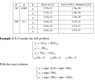
Table 3.2. Comparison of the absolute errors in the approximations obtained using the new class of methods, for instance (21), and the sixth-order method of Wu et al. [16] for Example 3.2.

T h Y Error of (21) Error of Wu’s Method in [16] 50 0.005

1

y 3.25e-21 1.38e-20

2

y 3.25e-21 1.38e-20

3

y 3.25e-21 1.38e-20

100 0.1

1

y 4.65e-32 3.57e-31

2

y 4.65e-32 3.57e-31

3

y 4.65e-32 3.57e-31

Example 3. 3. Consider the stiff problem

      

 

  

 

  

. 2 ) 0 ( , 1 ) 0 ( , 2 ) 0 (

, 120 70

, 50

, 9 . 49 1 . 0

3 2

1

3 2

' 3

2 '

2

2 1

' 1

y y

y

y y

y

y y

y y

y

With the exact solution

    

   

 

   

). 120 exp( ) 50 exp(

), 50 exp(

), 50 exp( ) 1 . 0 exp(

3 2 1

t t

y

t y

t t

y

This equation has been solved numerically for T 0.1 and T0.18 using exact starting values and the Wu’s method. In the numerical experiment, we take the step lengths

h 0.001 and h 0.01. In Table 3.3, we present the absolute errors at the end-point.

Table 3. 3. Comparison of the absolute errors in the approximations obtained using the new class of methods, for instance (21), and the sixth-order method of Wu et al. [16] for Example 3.3.

T h Y Error of (21) Error of Wu’s Method in [16]

0.1 0.001

1

y 4.61e-13 1.75e-7

2

y 5.78e-13 3.59e-8

3

y 6.35e-13 3.72e-8

0.18 0.1

1

y 2.89e-11 1.64e-5

2

y 6.31e-12 2.79e-7

3

Example 3.4. The following stiff initial value problem arose from a chemistry problem

    

 

 



 

 

, 2500

, 1000 013

. 0

, 2500 1000

013 . 0

3 1 '

3

2 1 2

' 2

2 1 2

1 2

' 1

y y y

y y y

y

y y y

y y

y

with initial value y(0)(0,1,1)T. We solve this problem at x2 and compare the results with those of Ismail methods [10] and SDBDF [7]. In Table 3.4, we present the absolute errors at the x2.

Table 3. 4. Comparison of the absolute errors in the approximations obtained using the new class of methods, for instance (21), Ismail methods [10] and SDBDF [7] for Example 3.4.

x

i

y Exact solution Error of (21) Error of Ismail methods [10] Error of SDBDF [7] 20

1

y -3.616933169289e-6 7.6e-19 8.2e-11 3.1e-9

2

y 9.815029948230e-1 2.4e-15 6.1e-6 1.8e-6

3

y 1.018493388244 9.3e-15 5.7e-6 5.7e-6

A

CKNOWLEDGEMENTS

The authors wish to thank the anonymous referees for their careful reading of the manuscript and their fruitful comments and suggestions.

R

EFERENCES

1. J. C. Butcher, A modified multistep method for the numerical integration of ordinary differential equations, J. Assoc. Comput. Math., 12, 124135, (1965). 2. Y. F. Chang and G. Corliss, ATOMFT: Solving ODEs and DAES using Taylor

series, Computers Math. Applic. 28 (10-12), 209233, (1994).

3. G. Dahlquist, A special stability problem for linear multistep methods, BIT, 3, 2743, (1963).

4. C. W. Gear, Hybrid methods for initial value problems in ordinary differential equations, SIAM J. Numer. Anal., 2, 6986, (1964).

5. C.W. Gear, Numerical solution of ordinary differential equations, SIAM Review

23, 1024, (1981).

7. E. Hairer and G. Wanner, Solving ordinary differential equation II: Stiff and Differential-Algebric Problems, Springer, Berlin, (1996).

8. H. J. Halin, The applicability of Taylor series methods in simulation, In Prec. 1983

Summer Computer Simulation Conference, July 1013, (1983).

9. P. Henrici, Discrete Variable Methods in Ordinary Differential Equations, John Wiley and Sons, 1962.

10. G. Ismail, and I. Ibrahim, New efficient second derivative multistep methods for stiff systems, J. Appl. Math. Model. 23, 279288, (1999).

11. J. D. Lambert, Computational methods in ordinary differential equations, John wiley and Sons (1972).

12. W. Liniger, R. A Willoughby, Efficient numerical integration of stiff systems of ordinary differential equations, Technical report RC-1970, Thomas J. Watson research center, Yorktown Heihts, N. Y. 1976.

13. A. Shokri, A. A. Shokri, The new class of implicit L-stable hybrid Obrechkoff method for the numerical solution of first order initial value problems, J. Comput. Phys. Commun., 184, 529531, (2013).

14. A. Shokri, M. Y. Rahimi Ardabili, S. Shahmorad, and G. Hojjati, A new two-step P-stable hybrid Obrechkoff method for the numerical integration of second-order IVPs., J. Comput. Appl. Math., 235, 17061712, (2011).

15. W. L. Miranker, Numerical Methods for Stiff Equations, p. 57, D. Reidel Publishing, Holland, (1981).

16. X. U. Wu and J.L. Xia, The vector form of a sixth-order A-stable explicit one-step method for stiff problems, Comput math. Applic. 39, pp. 247257, (2000).