Adaptive multi-scale shallow flow model: a
wavelet-based formulation
Georges Kesserwani
1*,Mohammad Kazem Sharifian
2†James Shaw
1 1 Civil & Structural Engineering, University of Sheffield, Sheffield S1 3JD, UK2 Department of Civil Engineering, University of Tabriz, Tabriz, Iran
Abstract
This work outlines the use of wavelet bases to re-formulate a finite volume (FV) local solution of the shallow water equations (SWEs), so as to achieve mesh adaptivity via local compression and truncation of the numerical solution’s details across successive resolution scales with reference to a single threshold error set by the user. The wavelet bases naturally lead to a scalable FV formulation and how they can readily be exploited to achieve adaptive mesh-resolution selection: up-scaling and/or down-scaling by means of the local solutions’ data (i.e. both flow variables and terrain). Our results show a notable promise in using wavelets as a basis for future flood models to achieve conservative and more autonomous simulation at a wide range of length-scales.
1
Introduction
Developing a scalable flow solver, i.e. in which model formulations, posed at multiple length scales, are automatically selected from a single and highly flexible simulation framework, has been a topic of both interest and contradiction to the hydroinformatics community (Haleem et al. 2005). While the community is keen on having a model that can smartly select and manage a cascade of scales in modelling inter/multi-regional flow processes/data, extrinsic forms of mesh adaptivity still lack an exhaustive strategy for data encoding and decoding across distinct mesh scales. In fact, these forms seem to give rise to controversial effects, e.g.: keeping a coarsest resolution that is fine enough, turning more input parameters for coarsening vs. refinement; in other words, offer little scope to simulate over a range of length-scales (e.g. when flow/terrain length-scales vary between cm and km), increase model sensitivity and problem-dependency, and impact the fidelity of the output.
Wavelet theory for local decomposition and reconstruction of (self-similar) functions offers a natural way of adaptively compressing and decomposing data. Recently, in Haleem et al. (2005) it has been demonstrated to be useable as a natural basis for re-formulating local piecewise-constant finite
* Created the first stable version of this document † Ran simulation test reported in this document
Volume 3, 2018, Pages 1040–1047
volume (FV) solutions of the shallow water equations (SWEs). However, the work in Haleem et al. (2005) did not entirely exploit and assess the local compression mechanism of wavelets (i.e. mesh refinement still relied on non-local gradient data, level of refinement was limited to 2 and a relatively fine coarse baseline mesh was still necessary to ensure reliable operation for the mesh refinement).
This contribution therefore presents an improved implementation that is entirely reliant on local (encoding and decoding of) wavelet coefficients in the adaptive modelling process, transfer and recovery of flow and terrain data, and in a manner that is entirely conservative of the practical features for solving the SWEs with topography and wetting and drying. To illustrate the relevance of the proposed approach for modelling over a significantly wide range of length-scales, a primary setting based on single-cell coarse mesh allowing for 9 levels of refinement is considered and explored in detail through a couple of well-known hydraulic test cases.
2
Haar wavelets
The Haar wavelets are constructed from a function , or a “father basis”, which takes unity over a
reference interval, i.e. [-1; 1], and is scaled by 2-1/2. The scaling function is orthonormal for the
norm defined by integration over [-1; 1] and is refinable (Keinert 2004). By translation and dilatation of , it is possible to define children scaling bases relevant to any resolution level (n), i.e. spanning non-overlapping sub-divisions (Ij)j, j = 0, 1, …, 2n-1, of the reference interval [-1; 1] in the
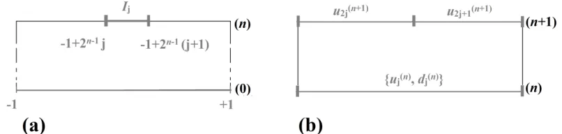
dyadic and recursive sense. On Ij (Figure 1(a)) a child basis can be defined, i.e. ,
, which preserves the properties of and has compact support ( ,
).
Figure 1 (a): sub-cell Ij at resolution (n) and (b) two-scale data relationships, i.e. Eq. (3)
On the other hand, the father basis allows to define a mother (Haar) wavelet , which actually
represents the encoded difference between , i.e. at level (0), and its two children at resolution level
(1); is supported on the same interval as , but clearly admits a discontinuity:
(1)
It is worth noting that this discontinuity property offers an advantage for the analysis of signals with sudden transitions such as those that potentially occurring in the case of shallow water modelling. Notable also, is a bi-orthonormal basis, thus also allowing to define children on (Ij)j, j = 0,
j
j
j
( ( )n)j j
j
( )n( ) 2n/ 2 ( )
j j
j x = j x
2 (n 1) 2 1
j j
x= x + - -
j
( )n( ) 0j l
j x =
l Il j
x Î ¹
j
y
j
y
j
1/ 2
1/ 2
2
[ 1;0]
( )
2
[0; 1]
x
y x
x
-ì-
Î
-ï
=
í
+
Î
+
ïî
y
( ( )n)j j
1, …, 2n-1 by translation and dilatation. For a fixed resolution level (n), can be interpreted as
the encoded difference between the scaling basis at level (n), i.e. and its two children at level
(n + 1), i.e. { }. This setting offers two interchangeable ways to describe a signal u(x) at a
level (n): a “single-scale” expansion by solely referring to the scaling bases , or a “multi-scale” expansion by referring to the father basis and the wavelet bases, as underlined in Eq. (2).
(2)
In (2), the scale, i.e. , and wavelet, or detail, coefficients, i.e. , are obtainable
by the dot product defined by integration over Ij (Keinert 2004, Haleem et al. 2015). The single-scale
form is useful to apply a numerical method for evolving scale-coefficients at a desired resolution levels (n). The multi-scale form decomposes the signal u(x) as the sum of a coarsest datum and its encoded details across higher resolutions, which are negligible if u(x) is smooth but become increasingly significant with increasing levels of non-smoothness in u(x), thereby offering the benefit to analyse u(x). Hence, the multi-scale form is useful to gain a natural mechanism for mesh-resolution adaptivity.
2.1
Adaptive and rigorous multi-scale setting
Through a user-specified threshold error , non-significant details in the multi-scale form of Eq. (2) can be truncated (i.e. zeroed), and this is the keystone of wavelet-based resolution adaptivity. By adding the remaining significant details (level-wise) to the coarse datum, i.e. via encoding, they enable the lifting of signal resolution up to the level required. Moreover, formulae for encoding and decoding can be produced, which offer rigorous means to alternate between the single-scale and multi-scale forms of the signal, as necessary (see also Sec. 4). For example, in Figure 1(b), the scale coefficients at a level (n+1) can be decoded to get both scale- and detail-coefficient at level (n), i.e. via Eq. (3a); whereas, Eq. (3b) allows to encode the scale-coefficients from (n) to (n+1).
(3a) (3b)
In (3a) and (3b), {h0, h1} and {g0, g1} represent the low-pass and high-pass filter bank coefficients, respectively, which are standard for the Haar wavelet and are well-documented in the literature (Keinert 2004).
3
Single-scale Finite Volume (FV) formulation for the SWEs
The hyperbolic balance law system (i.e. ∂tU + ∂xF = S) of the 1D SWEs considers a flow vector U =
(h, q)T, a flux vector F(U) = (q, q2 h-1 + 0.5g h2)T and a bed slope source term vector S = (0, -g h ∂xz)T;
h, q, g and z indicate the water depth (m), unit-width flow rate (m2/s), gravity constant (m/s2) and
topography (m), respectively. To solve the system by a finite volume approach over [xmin, xmax], it is
discretised into N(0) uniform cells (Ii = [xi-1/2, xi+1/2])i of size Δx(0) = xi+1/2 - xi-1/2 and centre xi = 0.5 (xi+1/2
+ xi-1/2). By posing ξ = 2(x-xi)/Δx(0), a cell Ii can be brought into [-1, 1]. Hence, it suffices to present
( )
( n )
j j
y
( )
( n )
j j j
( ) ( ) 2 , 2 1
n n
j j
j j
+( )
( n)
j j
j
( 1)
2 1 2 1
( ) ( ) (0) ( ) ( )
0 0 0
coarsest datum
single-scale details
multi-scale
( )
( )
( )
( )
n n lev
n n lev lev
j j j j j
j lev j
u
j
x
u x
u
j
x
-d
y
x
- -= = =
æ
ö
»
»
+
ç
÷
è
ø
å
å å
( )n , ( )n
j j
u =áuj ñ (lev) , (lev)
j j
d =áuy ñ
(
)
(
)
( ) 1/ 2 0 ( 1) 1 ( 1) 2 2 1 ( ) 1/ 2 0 ( 1) 1 ( 1)
2 2 1
2 h h
2 g g
n n n
j j j
n n n
j j j
u u u
d u u
+ + + + + + = + = +
(
)
(
)
( 1) 1/ 2 0 ( ) 0 ( )
2
( 1) 1/ 2 1 ( ) 1 ( )
2 1
2 h g
2 h g
n n n
j j j
n n n
j j j
u u d
u u d
+
+ +
= +
exploiting the compact-support and orthonormality properties of the scaling bases, and applying approximate integration means, the following single-scale discrete form is obtained:
(4)
In (4), stands for a Roe-based numerical flux function applied after revising the input arguments so as to achieve well-balanced positivity preserving Riemann states as in (Liang and Marche 2009). The latter were also applied in the evaluation of the source term vector S. The term Δx(n) = Δx(0)/2n
represents the size of a local sub-cell Ij. Explicit Euler time stepping is applied to discretise the LHS
term. The RHS term in (4) and the initial conditions, see Eq. (5), both re-scaled by a factor of 2n/2 2-1/2.
(5)
4
Adaptive mesh selection and update
Starting from the initial condition, in Eq. (5), its multi-scale version, in Eq. (2), is produced by recursive decoding, via (3a), and is followed by truncation of its non-significant details. By recursive encoding, via (3b), an adaptive mesh is made (i.e. a set encompassing single-scale coefficients from across various resolution levels) where the FV formulation, Eq. (4), is applied. After one time step update, decoding is applied again to enable restarting the overall process until reaching a desired output time. It is worth noting that the topography variable should also be included within the encoding and decoding processes to initiate and ensure that mesh resolution remains at the level required for capturing topographic features. For the threshold error, it should be chosen by the user such that 0 < < 1. The smaller the , the more detailed will the modelling be around smooth areas. One problem-dependent choice would be take proportional to the smallest-resolution feature
desired, i.e. with 0 < C ≤ 1, with for example C = 0.5 as a halfway compromise between
runtime efficiency and finest-resolution accuracy (i.e. ).
5
Some illustrative results
To illustrate the net benefit of the proposed Haar wavelets in FV (HFV) modelling of shallow flow, test cases are considered on a spatial domain [0, 50] that is discretised by a coarse background mesh made of a single cell, i.e. N(0) = 1, and allowing up to 9 levels of resolution-refinement, equivalent to a
mesh containing 29 = 512 cells. For this setting, the threshold error recommended in Sec. 4 would be
= 0.0488, which will be considered together with other possible values such as = 0.1, 0.01 and 0.001 to allow more systematic exploration of the response of the HFV adaptive scheme in relation to the choice of the threshold error.
5.1
Well-balanced property with wet-dry zones
This first sub-test is designed to demonstrate that the adaptive HFV scheme: (i) effortlessly inherits the properties of the reference FV scheme in terms of well-balanced property with wetting and/or drying over uneven topography, and (ii) can be used as a direct mechanism for autonomous mesh generation within the process. The sub-test considers a quiescent flow interacting with complex and different topography shapes over the domain, which were designed to span different levels of smoothness, kinks and discontinuities that could be observed in realistic applications. The initial
conditions (h + z = 2 m and q = 0 m2/s) were chosen in a manner to consider scenarios with a
fully-(
1) (
1)
(
)
( ) ( ), ( ), ( ), ( ), ( ) ( )
1 1
( )
1 ( , ), ( , ) ( , ), ( , ) ( , )
j j j j j j
n n n n n n n
t I xn I xj t I+ xj t I- xj t I xj t x I xj t
+ - +
-+
-é ù
¶ =- ë - - D û
D
U F U U F U U S U
F
(
)
(
)
( ) 1 1 1
0 0 0
2
(0) 1 2 1 2 ( 1) with ( ) given at 0 j
n n n
I j
U = é - + - j + - + - j+ ù x t = s
ëU U û U
e
e
e
( )n
C x
e » D
0.04488
e »
wet domain (h > 0), a critically dry portion (h = 0) and a fully dry portion where the water level cuts through a dry obstacle (h < 0), with the terrain shapes following:
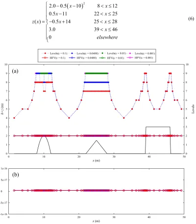
(6)
Figure 2 Still water state over uneven terrain (black lines): (a) free surface elevation and (b) discharge.
Simulations are carried out for a relatively long time evolution, i.e. 100 s, considering the selected values for the threshold error, i.e. = 0.1, 0.01, 0.04488 and 0.001. The results for all these choices for the threshold error show zero discharge up to machine precision (see Figure 2b) and unperturbed steady state for the free-surface elevation (see Figure 2a). This clearly indicates that the adaptive HFV
(
)
22.0 0.5 10 8 12
0.5 11 22 25
( ) 0.5 14 25 28
3.0 39 46
0
x x
x x
z x x x
x elsewhere
ì - - < £
ï
- < £
ï ï
=í- + < £
ï < £
ï ïî
x (m)
0 10 20 30 40 50
h+
z
(m)
0 1 2 3 4 5 6 7 8 9 10
L
eve
ls
0 1 2 3 4 5 6 7 8 9 10 Levels(e = 0.001)
Levels(e = 0.01) Levels(e = 0.0488)
HFV(e = 0.01) HFV(e = 0.001) HFV(e= 0.0488)
HFV(e = 0.1) Levels(e = 0.1)
x (m)
0 10 20 30 40 50
q
(m
2 /s)
-1e-16 -5e-17
0 5e-17 1e-16
(a)
(b)
wet/dry zones and fronts, suggesting that the introduction of the wavelet into FV scheme to achieve adaptive multi-resolution modelling would not lead to any spurious noise.
In terms of impact of the choice of the threshold error, it is mostly apparent in the resolution level selections (Figure 2a), which herein is entirely driven by the terrain features, as it should be given the lake at rest conditions for the flow variables. As expected, for smaller threshold errors, i.e. = 0.01 or 0.001, the adaptive HFV scheme over-refines at mildly smooth areas (i.e. at the humps in Figure 2a around x = 10 m and x = 25 m) where the highest resolutions are taken to represent the whole terrain obstacles. In contrast, for larger threshold errors (i.e. = 0.0488 and 0.1) lower resolution levels are predicted by the scheme for representing these obstacles. Most notably, when terrain discontinuities are sharp (e.g. Figure 2a, around x = 45 m) all the selected values seem to appropriately predict a mesh that has the finest resolution solely restricted at the sharp edges. These results therefore suggest that all the explored threshold error values can be feasible for modelling water flow over topography, and whether to increase or decrease the value of the threshold error seems to be dependent on the resolution precision desired by a user to better resolve for smooth topographic features.
5.2
Transient dam-break flow
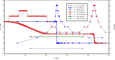
This second sub-test considers an idealised dam break flow over flat terrain with a view to solely explore the ability of the proposed adaptive HFV scheme in deciding mesh-resolution when various types of nonlinear discontinuities (i.e. a shock and depression wave) are present, and in track with their transient nature. The domain is now assumed to have an imaginary dam located in its middle (i.e. x = 25 m) separating two initial water levels of 6 m and 4 m located upstream of and downstream of the dam, respectively. At t = 2.5s, the incident dam break wave (based on an available analytical profile, which is illustrated in Figure 3) is expected to produce a shock wave travelling downstream and a rarefaction wave propagating upstream, which are separated by an intermediate constant water state. After certain time evolution, e.g. t > 40s, and assuming slip boundary conditions, the water level in the domain should become constant as the shock and rarefaction waves should already have propagated outside it. In line with these expected observations, the adaptive HFV scheme is run considering, firstly, the problem-dependent threshold error = 0.04488 and its results at t = 0, 2.5 s and 40s are shown below in Figure 3.
Figure 3 Dam-break depth profiles and associated
resolution levels at different output times ( ). Figure 4 Idealised dam break (numerical results using different threshold errors. t = 2.5 s), comparison of
At t = 0 s, the adaptive HFV scheme predicted a mesh considering the highest resolution level at the discontinuity, but showing gradual reduction in resolution levels elsewhere up to having very coarse levels at the boundaries. At t = 2.5 s, the numerically predicted dam-break profile follows closely the analytical solution, however on a mesh where resolution levels are highest at the shock, slightly coarser around the rarefaction, and lowest at the constant water state between them. At t = 40 s, the resolution level predicted by the adaptive scheme boils down to “1”, which seems to be sensible
e
e
e
e
x (m)
0 10 20 30 40 50
L ev els 0 1 2 3 4 5 6 7 8 9 10 h+z (m) 0 1 2 3 4 5 6 7 8 9 10
T = 2.5s (Exact) T = 0s (Num.) T = 0s (Levels) T = 2.5s (Num.) T = 2.5s (Levels) T = 40s (Num.) T = 40s (Levels)
x (m)
0 10 20 30 40 50
L ev els 0 1 2 3 4 5 6 7 8 9 10 h+z (m) 0 1 2 3 4 5 6 7 8 9 10 Exact Num. (e = 0.001) Lev. (e = 0.001) Num. (e = 0.01) Lev. (e = 0.01) Num. (e = 0.1) Lev. (e = 0.1)
0.04488
as the flow became free from any discontinuity as the shock and rarefaction disappeared from the domain by this time. These results indicate that the present HFV adaptive scheme is able to automate sensible decision-making for the resolution levels in keeping with the flow transients and discontinuities and without being affected by the utmost level of coarseness in the baseline mesh.
Secondly, to further explore accuracy and efficiency issues related to the choice of the threshold error values, adaptive HFV runs are now considered for the output time t = 2.5 s, but considering instead the threshold errors = 0.1, 0.01, and 0.001. Figure 3 compares the associated numerical profiles produced by the scheme with the analytical solution. As expected, given the observation in Sec. 5.1, all the schemes predict the highest mesh resolution possible at the shock, irrespective of the threshold error selected. At the rarefaction, however, the bigger the threshold error, the coarser the level of resolution predicted, with clearly diffusive results for the choice = 0.1 and over-refinement for = 0.001. At the constant state, the mesh predictions made by = 0.01 and 0.1 are the same whereas finer resolution levels were triggered for = 0.001. Therefore, for highly transient flow problems involving smooth discontinuities it can be concluded that a threshold value between 0.01 and 0.1, e.g. the suggested problem-dependent value of 0.04488, should be enough to avoid over-prediction and thereby achieve a reasonable compromise among resolution accuracy and efficiency. To also provide an idea on efficiency gain relating to the choice of threshold error, a run was performed on a uniform mesh considering 512 cells, i.e. the highest resolution accessible by the adaptive scheme.
Threshold error (e) Approx. CPU time (s) Speed-up (X)
Uniform mesh Adaptive mesh
0.1 70 23 3.0
0.01 70 31 2.2
0.001 70 36 1.9
Table 1 CPU time for dam break case (t = 2.5 s) for the standard setting considered (N(0) = 1, n = 9)
{N(0), n} scenarios Approx. CPU time (s) Speed-up (X)
Uniform mesh Adaptive mesh
{1, 9} 70 36.0 1.94
{2, 8} 70 36.8 1.91
{4, 7} 70 36.9 1.89
{8, 6} 70 39.0 1.79
{16, 5} 70 44.0 1.59
{32, 4} 70 47.2 1.48
{64, 3} 70 60.0 1.16
Table 2 CPU time for dam break case (t = 2.5 s and = 0.001). Different scenarios for the choice of the number of cells for the baseline mesh vs. maximum depth of resolution levels, i.e. {N(0), n}.
Table 1 lists the approximate CPU times generated by the adaptive mesh runs and the uniform mesh run. As expected, the lower the threshold error, the less the speed-up, which seems to be around 1.9-3X for this test relative to the uniform mesh counterpart (to achieve a simulation for 2.5 s). However, it might be worth further exploring the speed-up for longer runtimes and/or other tests where the impact-event features constitute a relatively small portion of the domain to get a more realistic picture on the efficiency gain of the adaptive HFV scheme.
Finally, this test case is re-explored (i.e. for the output time t = 2.5 s and considering only = 0.001) with a view to analyse potential sensitivity issues related to coarseness of the baseline mesh, i.e. N(0). Therefore, simulations are re-run considering a range of scenarios by tuning {N(0), n} such
that the finest-resolution accessible remains constant (i.e. equivalent to a uniform mesh of 512 cells).
e
e
e
e
e
e
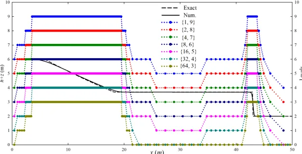
Figure 5 Idealised dam break (t = 2.5 s). Different scenarios for the choice of the number of cells for the baseline mesh vs. maximum depth of resolution levels, i.e. {N(0), n}.
This was achieved by choosing variants of the HFV scheme by recurrently doubling the number of baseline mesh cells, i.e. N(0), and reducing by one the maximum level of resolution, i.e. n. Table 2
(above) lists the scenarios considered, their CPU runtime costs and speed-up relative the uniform mesh counterpart on a mesh with 512 cells. Their related simulation results are illustrated in Figure 5 (below). Interestingly, despite the increase in N(0), all the variants predicated similar patterns for the
mesh resolution, hence yielding similar results in terms of overall resolution accuracy considering both baseline mesh and the depth in resolution levels (for this reason, only one numerical results was included in Figure 5 relative to scenario {2, 8}). In contrast, a drop is noted in the relative efficiency speed-up in line with the increase in N(0), i.e. from around 1.9X with scenario {1, 9}, which involved a
single-cell baseline mesh, down to 1.1X with scenario {64, 3} involving a 64 cells in the baseline mesh. These findings seem to suggest that HFV method is able to automate resolution refinement even while taking the coarsest baseline mesh possible, i.e. 1 cell, and at the same level of precision of any other variant involving more cell in the baseline mesh. They also clearly indicate that the adaptive
mechanism involved in the HFV method is more efficient with decreasing N(0) and despite increasing
n (i.e. less costly when called less times but with more depth in the refinement levels, rather than more times but less deep refinement levels). Therefore, it makes sense, based on these preliminary results, to favour an adaptive HFV setting that involves as coarse as possible resolution in the baseline mesh, and as deep refinement levels as needed/affordable.
Acknowledgements
This work was supported by the EPSRC grant EP/R007349/1.
References
F. Keinert, Wavelets and Multiwavelets, CRC Press, Florida, USA (2003).
D. Haleem, G. Kesserwani, D. Caviedes-Voullième, Haar wavelt-based adaptive finite volume shallow water solver, J. Hydroinf. 17 (2015) 857–873.