ISSN: 2008-6822 (electronic)
http://dx.doi.org/10.22075/ijnaa.2017.415.1060
Numerical algorithm for pricing of discrete barrier
option in a Black-Scholes model
Rahman Farnoosha,∗, Hamidreza Rezazadehb, Amirhossein Sobhania, Masoud Hassanpourc
aSchool of Mathematics, Iran University of Science and Technology, 16844 Tehran, Iran bDepartment of Mathematics, Karaj Branch, Islamic Azad University, Karaj, Iran
cDepartment of Mathematics, Faculty of Mathematics, Statistics and Computer Science, Semnan University, Semnan, Iran
(Communicated by M. Eshaghi)
Abstract
In this article, we propose a numerical algorithm for computing price of discrete single and double barrier option under theBlack–Scholes model. In virtue of some general transformations, the partial differential equations of option pricing in different monitoring dates are converted into simple diffusion equations. The present method is fast compared to alternative numerical methods presented in previous papers.
Keywords: Discrete barrier option, Black–Scholes model, Constant parameters. 2000 MSC: Primary 47H10, 47H09; Secondary 54H25, 55M20.
1. Introduction
Option pricing is one of the most important problems in quantitative finance and many researchers are involved in it. As a description, down–and–out barrier option is that option which deactivated (knock–out) if the price of underlying asset touches the predetermined barrier. In practice and with attention to academic literature, barrier options have been studied under two discrete and continuous monitoring. In the first case, the price of underlying asset has been checked at predetermined monitoring dates. The price of underlying assets is usually modeled as geometric Brownian motion process where the model parameters are constants.
In the present paper, we try to price a down–and–out discrete single and double barrier option on an underlying asset which is modeled as geometric Brownian motion with constant parameters. In
∗Corresponding author
Email addresses: [email protected](Rahman Farnoosh), [email protected]( Hamidreza Rezazadeh),[email protected], [email protected](Amirhossein Sobhani),
[email protected](Masoud Hassanpour)
this regard, a set of transformations are applied to correspond partial differential equations (PDEs) for option price. Afterwards, the obtained PDEs are simply converted to familiar heat equations whose solutions are as multiple integral forms. Finally, a new numerical method is proposed to accurately computation these multiple integrals.
This article is managed as follows. In Section 2, the model structure for pricing discrete down– and–out single and double barrier options is discussed and a recursive method is presented. In Section 3, a numerical algorithm is proposed to evaluate the multiple integral in section 2. In addition, we compare the obtained results in the present paper to the alternative numerical methods in other papers for pricing discrete barrier options like [15] and [17]. At last, obtained conclusions and remarks are offered in Section 4.
2. Discrete barrier option modeling in the Black–Scholes world model
In this section, we focus on pricing discrete down–and–out call option and both down–and–out, up– and–out hedging on a underlying stock which could be expired its worth if a lower or upper barrier touches the continuous path of stock value at predetermined monitoring dates. At first we define some preliminary concepts. With attention to this fact that the summation of in and out call option price (in each case down or up) is equal to the price of a simple European call option [20, 21]. Other kind of barrier options like as down–and–out put option, could be priced using the put call parity given in[12]. Also we suppose that the price of underlying stock, that we denote it with Xt, is a Geometric Brownian Motion process, i.e.
dXt=µXtdt+σXtdWt, X0 =x0,
where Wt is Wiener process, X0 = x0 is stock price in initial time t = 0 and three deterministic
constant valuesD, ρ=µ−Dand σ, are non–dividend–paying equity, drift and the time independent
instantaneous volatility respectively. For more details about SDEs and its application, especially in mathematical finance, refer to [14], [8] and [16].
2.1. Black–Scholes PDE for single barrier option pricing
In all over our discussion, we consider 0 = t0 < t1 < . . . < tn < . . . < tN =T the monitoring dates. The price of down–and–out call barrier option with the strike price K and lower barrier L, that is active in all monitoring dates tn, is denoted by B(x, t, n)≡ B(x, t, n;L). So B(x, t, n) satisfy in the
well–known Black–Scholes PDE with relevant initial conditions:
−∂B(x, t, n) ∂t +µx
∂B(x, t, n) ∂x +
1 2σ
2x2∂ 2
B(x, t, n)
∂2x −µB(x, t, n) = 0, (2.1)
B(x, t0,0) = (x−K)1(x≥max(K,L)); n = 0, (2.2)
B(x, tn, n) = B(x, tn, n−1)1(x≥L); n= 1,2, . . . , N −1, (2.3)
whereB(x, tn, n−1) is defined as B(x, tn, n−1) :=limt→t−nB(x, t, n−1) and 1(x≥L) is characteristic
function. Keeping away from making other symbols, we attempt to infer a way to reach the suitable option pricing for discrete barrier in monitoring dates.
compare it with other implemented methods applied in [9]. After applying the following transforms in each separate time interval:
B(x, t, n) =B(Z, t, n), Z =ln
x L
, k=ln
K L
, (2.4)
and rearranging (2.1), based on well–known converterB(Z, t, n), a new PDE is concluded:
−∂B
∂t +m ∂B
∂Z + σ2
2 ∂2B
∂Z2 −µB= 0, (2.5)
thatm=µ−σ2/2, and according to the last conversion the initial condition (2.2) and (2.3) converts to following condition:
B(Z, t0,0) = L(eZ −ek)1(Z≥δ), δ= max{k,0} (2.6)
B(Z, tn, n) = B(Z, tn, n−1)1(Z≥0), n = 1,2, . . . , N −1. (2.7)
By following transform
B(Z, t, n) =eαZ+βtg(Z, t, n), n= 0,1,2, . . . , N −1, (2.8)
where αandβ are defined as
α=−m
σ2, β =αm+α 2σ2
2 −µ, (2.9)
we reach the Heat equation
−∂g
∂t +C
2∂2g
∂Z2 = 0, C 2
= σ
2
2 , n = 0,1,2, . . . , N −1. (2.10) In addition, the initial conditions (2.6) and (2.7) convert to following
g(Z, t0,0) = Le−α0Z(eZ−ek)1(Z≥δ), δ= max{k,0}, (2.11)
g(Z, tn, n) = g(Z, tn, n−1)1(Z≥0), 1≤n≤N −1 (2.12)
which has unique analytical solution in each time interval [tn, tn+1] (see[19]):
g(Z, t, n) = L Z ∞
0
Sn(Z−ξ, t−tn)e−αξ(eξ−ek)1(ξ≥δ)dξ , n= 0, (2.13)
g(Z, t, n) = Z ∞
0
Sn(Z −ξ, t−tn)g(ξ, tn, n−1)1(ξ≥0)dξ , n= 1,2, . . . , N −1. (2.14)
In above equality kernel S(Z, t), is the normal distribution function N0,√4C2t
Sn(Z, t) = 1
√
4πC2texp
−Z2 4C2t
, n = 0,1,2, . . . , N −1. (2.15)
According to the concluded results, the price of the discrete barrier option at monitoring dates tn, can be calculated by following theorem.
Theorem 2.1. The price of down–and–out discrete barrier call option with stock price x, strike price K, and barrier levelL, at monitoring dates tn+1, are evaluated as follow
B(x, tn+1, n) =g
ln(x
L), tn+1, n
exp{αln(x
L) +βtn+1}, n = 0,1,2, . . . , N −1, (2.16) where the constants α and β are defined in (2.9) and g(., tn+1, n) is evaluated recursively in (2.13)
2.2. Black–Scholes PDE for double barrier option pricing
In this subsection, the price of down–and–out and up–and–out call double barrier option with the Strike price K, the constant lower and upper barrier L1 and L2, is denoted by DB(x, t, n) ≡ DB(x, t, n, L1, L2). The double barrier option priceDB(x, t, n), under theBlack–Scholes world
frame-work satisfy in the well–knownBlack–Scholes PDE
−∂DB(x, t, n)
∂t +µx
∂DB(x, t, n) ∂x +
1 2σ
2x2∂ 2
DB(x, t, n)
∂2x −µDB(x, t, n) = 0, (2.17)
with these initial conditions
DB(x, t0,0) = (x−K)1(L2≥x≥max(K,L1)); n = 0, (2.18)
DB(x, tn, n) = DB(x, tn, n−1)1(L2≥x≥L1); n= 1,2, . . . , N −1, (2.19)
whereDB(x, tn, n−1) is defined asDB(x, tn, n−1) :=limt→t−nDB(x, t, n−1). By applying following
transform
¯
DB(¯x, t, n) =DB(Z, t, n), Z =ln(
¯ x L1
), k =ln(K L1
) (2.20)
and rewriting PDE (2.17) and initial conditions (2.18), based on DB(Z, t, n), we have
−∂DB
∂t +m ∂DB
∂Z + σ2
2
∂2DB
∂Z2 −µDB = 0, (2.21)
DB(Z, t0,0) =L1(eZ−ek)1(ln(L2 L1)≥Z≥δ)
, δ = max{k,0} (2.22)
DB(Z, tn, n) =DB(Z, tn, n−1)1(ln(L2 L1)≥Z≥0)
, n = 1,2, . . . , N −1, (2.23)
where m=µ−σ2/2. Another conversion as follow is done in each time interval
DB(Z, t, n) = eαZ+βtg(Z, t, n), n = 0,1,2, . . . , N −1, (2.24)
which α and β are defined by (2.9). After rewriting PDE (2.21) respect to g(Z, t, n), we obtain the Heat equation:
−∂g
∂t +C
2∂2g
∂Z2 = 0, C 2 = σ2
2 , n = 0,1,2, . . . , N −1, (2.25) also the initial conditions (2.22) and (2.23) convert to following
g(Z, t0,0) =L1e−α0Z(eZ−ek)1(ln(L2 L1)≥Z≥δ)
, δ= max{k,0}, (2.26)
g(Z, tn, n) =g(Z, tn, n−1)1(ln(L2 L1)≥Z≥0)
. (2.27)
These are as well–known second order PDEs which have unique analytical solution in each time interval [tn, tn+1] as follows [19]
g(Z, t, n) =L1
Z ∞
0
Sn(Z−ξ, t−tn)e−αξ(eξ−ek)1(ln(L2 L1)≥ξ≥δ)
dξ, n= 0, (2.28)
g(Z, t, n) = Z ∞
0
Sn(Z−ξ, t−tn)g(ξ, tn, n−1)1(ln(L2 L1)≥ξ≥0)
dξ, n= 1,2, . . . , N −1. (2.29)
Theorem 2.2. The price of down–and–out, up–and–out double discrete barrier call option with stock price x, strike price K, and barrier levels L1 and L2, at monitoring dates tn+1, are evaluated
as follows
DB(x, tn+1, n) =g
ln( x
L1
), tn+1, n
exp{αln( x L1
) +βtn+1}, n = 0,1,2, . . . , N −1, (2.30)
where the constants α and β are defined in (2.9) and g(., tn+1, n) is evaluated recursively by (2.28)
and (2.29).
3. Numerical algorithm and some numerical results
In this section, a fast numerical algorithm for computing price of double and single barrier option with discrete monitoring dates, based on romberg numerical integration method, is presented. Assume that stock priceZ0 is given, we intend to evaluateg(Z0, t, N) as the price of discrete double barrier option.
Recursive formula (2.13) shows that for this purpose, dependent on numerical integration method that is implemented, we must evaluate g(., tN, N −1) in adequate points belong to [0,∞) but S function has exponential decay property and its maximum occurs inZ0, so we could consider integral
over finite interval IN−1 = [0, Z0 +l] instead of [0,∞) where l is chosen as large enough constant.
In similar way to compute g(ξ, tN, N −1) where ξ ∈ [0, Z0 +l], we must compute g(., tN−1, N −2)
in adequate points of the interval IN−1 = [0, Z0 + 2l]. By following this process, finally to evaluate
g(ξ, t2,1) where ξ∈[0, Z0+ (N −1)l], we have to evaluate g(ξ, t1,0) over I0 = [0, N l].
Note that in application we can considerIn= [0,min{(N −n)l, H}] that H is a practical constant. The algorithm for double barrier option is similar and it is just enough consider all integral interval [0,ln(l1/l2)]. The semi–code of this algorithm is as follows:
________________________________________________________________
Algorithm: Single barrier option pricing with N discrete monitoring dates
________________________________________________________________
Input:I m ∈Npositive integer, N ∈N number of monitoring dates
Output:J X ∈R+, option price.
1 step←0
2 numnode1 ← 2m.Ceil(length(I0)) + 1
3 h ← length(I0)/numnode1
4 for i= 0 : numnode1 do
5 ξi ← i.h 6 end
7 for i= 0 : numnode1 do
8 Compute g(ξi, t1,0) by gaussian quadrature rule.
9 end
10 for step= 1 :N −2 do
11 numnodestep ← 2m.Ceil(length(Istep)) + 1 12 h← length(Istep)/numnodestep
13 for i= 0 :numnodestep do
15 end
16 for i= 0 :numnodestep do
17 Compute g(ξi, tstep, step−1)by Romberg method based on Simpson0s rule using nodal points g(ξj, tstep−1, step−2), 0≤j ≤numnodestep−2.
18 end
19 end
20 X ← g(z0, tN, N −1)by Romberg method based on Simpson0s rule using nodal points g(ξj, tN−1, N −2), 0≤j ≤numnodeN−2.
Example 3.1. Consider the problem of pricing down–and–out discrete barrier call option on stock for different levels of L, maturity time T, and monitoring dates. The employed parameters in this example are stock price = 100, strike = 100,µ= 0.1,σ= 0.3, andT = 0.2 [9]. In Table 1, the pricing of a single barrier down–and–out call option for lower level L and different monitoring dates N has been presented. Also, the other methods which have been brought in this sample are the recursive integration method (RI) in [1] with 2000 used points; the continuous monitoring formula(CC) with the barrier level shifting which has been demonstrated in [7]; Trinomial tree method (TT) indicated in [6]; Monte Carlo (MC) in [3]. The Wiener–Hopf method (WH) is an analytical solution of discrete barrier option pricing [9].
Table 1: Discrete barrier option pricing of Example 3.1: µ= 0.1, σ2= 0.09
N L Presented Method AS RI CC TT Monte Carlo
5 89 6.2807 6.2807 6.2763 6.284 6.281 6.28092 5 95 5.6711 5.6711 5.6667 5.646 5.671 5.67124 5 97 5.1672 5.1672 5.1628 5.028 5.167 5.16739 25 89 6.2097 6.2099 6.2003 6.210 6.210 6.21059 25 95 5.0812 5.0814 5.0719 5.084 5.081 5.08203 25 97 4.1159 4.1158 4.1064 4.113 4.115 4.11621
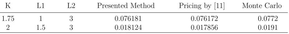
Example 3.2. Consider an especial case of discrete double barrier option with constant drift and volatility which has been mentioned in [11]. Consider the problem of pricing down–and–out and up–and–out discrete double barrier call option on stock for different levels of L and U, maturity time T = 1, and monitoring dates. The parameters are Stock price=2, µ(t) = 0.05, and σ2 = 0.5.
Obtained results are demonstrated in Table 2.
Table 2: Double Discrete Barrier option contract pricing of Example 3.2: µ= 0.05, σ2= 0.5
K L1 L2 Presented Method Pricing by [11] Monte Carlo
4. Conclusions and remarks
In this article, pricing of double and single discrete double barrier option under the Black–Scholes model with constant parameters, is investigated. The partial differential equations of option pricing in different monitoring dates are converted into simple diffusion equations and a fast numerical algorithm is presented. The accuracy of the numerical results shows the reliability and validity of this algorithm.
References
[1] F. AitSahlia and T.L. Lai,Valuation of discrete barrier and hindsight options, J. Financial Eng. 6 (1997) 169–177. [2] C.F. Baum, An Introduction to Modern Econometrics Using Stata, Stata Press, 2006.
[3] M. Bertoldi and M. Bianchetti, Monte Carlo simulation of discrete barrier options, Financial engineering– Derivatives Modelling, Caboto SIM Spa, Banca Intesa Group, Milan, Italy 25.1 (2003).
[4] F. Black and M. Scholes,The pricing of options and corporate liabilities, J. Political Economy 81 (1973) 637–659. [5] G.E. Box, P. Jenkins and G.M. Reinsel, Time Series Analysis: Forecasting and Control (3rd edition), Upper
Saddle River, NJ: Prentice–Hall, 1994.
[6] M. Broadie, P. Glasserman and S. Kou, A continuity correction for discrete barrier options, Math. Finance 7 (1997) 325–349.
[7] M. Broadie, P. Glasserman and S. Kou, Connecting discrete and continuous path–dependent options, Finance Stochast. 3 (1999) 55–82.
[8] L.C. Evans,An Introduction to Stochastic Differential Equations, Vol. 82. American Mathematical Soc., 2012. [9] G. Fusai, D. Abrahams and C. Sgarra,An exact analytical solution for discrete barrier options, Finance Stochast.
10 (2006) 1–26.
[10] G. Fusai and M.C. Recchioni, Analysis of Quadrature Methods for Pricing Discrete Barrier Options, J. Econ. Dyn. Control 31 (2007) 826–860.
[11] H. Geman and M. Yor, Pricing and hedging double–barrier options: A probabilistic approach, Math. Finance 6 (1996) 365–378.
[12] E.G. Haug, Barrier put–call transformations, Tempus Financial Engineering, Norway, download at http://ssrn.com/abstract 3 (1999) 150–156.
[13] R.C. Heynen and H.M. Kat,Look back options with discrete and partial monitoring of the underlying price,Appl. Math. Finance. 2 (1995) 273–284.
[14] A. Ludwing,Stochastic Differential Equations: Theory and Applications, Wiley, 1974.
[15] A. Ohgren,A remark on the pricing of discrete look back options, J. Comput. Finance 4 (2001) 141–146. [16] B. Oksendal,Stochastic Differential Equations, Springer, Berlin, Heidelberg, 65–84, 2003.
[17] G. Petrella and S.G. Kou,Numerical pricing of discrete barrier and look back options via Laplace transforms, J. Comput. Finance 8 (2004) 1–38.
[18] M.B. Priestley,Non–linear and Non–stationary Time Series Analysis, Academic Press, 1988. [19] W.A. Strauss,Partial Differential Equations: An Introduction, Wiley, NewYork, 2007.
[20] P. Wilmott,Derivatives: The Theory and Practice of Financial Engineering, Wiley, Chichester, 1998.