AUT J. Civil Eng., 2(2) (2018) 195-208 DOI: 10.22060/ajce.2018.14330.5472
The evaluation of the Friction Demand Factor in Loop Ramps of Interchange Facilities
M. H. Dehshiri Parizi, M. Tamannaei*, H. HaghshenasDepartment of Transportation Engineering, Isfahan University of Technology, Isfahan, Iran
ABSTRACT: The aim of this study is to evaluate the side friction demand factor in the loop ramps of interchange facilities. The substantial exclusivity of these ramps is the existence of horizontal curves, combined with longitudinal grades. In this study, CarSim and TruckSim software packages, as simulation tools, are applied. Both passenger cars and heavy vehicles are used. The vehicles used in simulations were Hatchback and Sedan (as passenger cars) and Truck (as heavy vehicle). In addition, two various types of loop ramps, including Curve-Curve-Curve and Spiral-Curve-Spiral, in two different conditions (braking and no-braking) are examined. The results showed that the side friction demand factor values assumed by AASHTO Green book (as a main geometric design guideline) are uncertain. In the condition of no-braking, the differences between AASHTO values and the simulation results for uphill and downhill states are 24% and 18%, respectively. In braking condition, similar differences for uphill and downhill are 124% and 135%, respectively. Additionally, based on the regression analysis of the simulation results, the appropriate side friction demand factor models were achieved for different conditions. The findings of the study verify the necessity of revising the friction demand values, especially for the design of interchange loop ramps.
Review History:
Received: 16 April 2018 Revised: 11 August 2018 Accepted: 15 August 2018 Available Online: 25 August 2018
Keywords:
Point-mass model Multi-body simulation Friction demand factor Loop ramps
CarSim TruckSim
1- Introduction
The side friction factor between tire and pavement is considered as an important safety parameter, which can affect the rate of vehicle crashes [1]. This parameter is defined as the ratio of the horizontal force to the vertical force [2]. The side friction demand factor is the amount of friction coefficient that vehicle needs to stabilize [3]. In order to design the horizontal curves, conventional geometric design guidelines [4] recommended the friction demand factors, by using a simple mathematical model called Point Mass (PM). In this model, the vehicle is represented as a Point Mass (PM). Due to the simplified assumptions of PM model, no consideration is given to the distribution of frictional forces between different tires of a vehicle. Although the application of PM model for the design of the simple horizontal curves can prepare sufficient margin of safety against both skidding and roll over, the model has serious limitations especially for the design of the facilities, which have combinations of the horizontal curve and longitudinal grades. Loop ramps are considered as one of such facilities. In AASHTO Green book, which is based on PM model, the designs for the alignment plan and the profiles are executed in separate procedures. Therefore, the use of AASHTO Green book seems not to be sufficient for the mentioned facilities. To cover the shortages of the PM model, vehicle dynamic models such as multi-body
model are developed. These models are regarded as a basis for simulation analysis, which evaluates vehicle stability on 3-D alignments.
The aim of this study is to evaluate the friction demand factor in loop ramps of the interchange facilities. The main contribution of this paper is to determine the required side friction demand factor in loop ramps, through a simulation-based methodology. CarSim and TruckSim software packages, which are based on the multi-body models, are employed as simulation tools. These software packages are able to animate the vehicle performance and plot the diagrams. In addition, we have investigated relationships between the friction demand factor and different parameters used to design the loop ramps of the interchange facilities.
The outline of the paper is as follows: in section 2, the background of vehicle stability models is explained. The methodology is described in section 3. The results of the simulation are presented in section 4. Finally, the concluding remarks are given to summarize the contribution of the paper. 2- Background
Starting in the late 1940s, friction factor studies were established, regarding the driver’s comfort [6]. Based on vehicle stability analysis, different methods such as point mass model, bicycle model, and multi-body simulation were presented [5, 7, 8]. Application of each of the mentioned models is related to their easiness and the accuracy required. Brief descriptions of each of the vehicle stability models are
presented in the following section. 2- 1- Point mass model
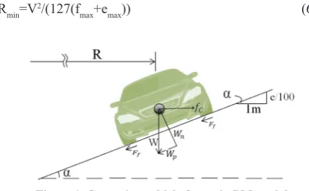
The Point Mass (PM) model is the most popular vehicle stability analysis, which has been used in conventional geometric design guidelines. PM model considers a cornering vehicle as a rigid and un-sprung mass in which dimensions of vehicle body do not have any effect on vehicle behavior [9, 10]. PM model is obtained from logical mathematics equations and simulates the vehicle motion with the main assumption that all forces entered a vehicle are concentrated at one point. The main features of this model are the ease of use and consideration of truck as a passenger car [5]. The cornering vehicle in point mass model undergoes centripetal acceleration. Centrifugal force causes the vehicle to skid and roll over and is neutralized by a combination of the side friction force and the weight force contributed by the exertion of super-elevation [11, 12]. The PM model employs the following calculations:
(1)
m.ar=∑Fy (2)
(3)
(4)
(5) The above parameters are defined as follows: ar centrifugal acceleration, V velocity, R radius curve, W weigh of the vehicle, α super-elevation angle, f side friction factor between tire and pavement surface, g gravity of earth and e super-elevation.
AASHTO Green book [4] defines equation of point mass, as follows:
Rmin=V2/(127(fmax+emax)) (6)
Figure 1. Cornering vehicle forces in PM model
Where fmax and emax are the maximum side friction demand factor and the maximum super-elevation, respectively. According to logics of Equation. 6, fmax is computed by safety factors and driver comfort. The friction demand is a function of roadway type, road surface conditions, and conditions of tire [5, 8]. In Figure. 2 , the side friction demand factor assumed in AASHTO Green book is illustrated.
According to point mass model, the cornering vehicle will not be able to stabilize if the friction demand exceeds friction supply. In other words, if the friction supply factor is not adequate, the vehicle will be skidding out of the curve [2, 11]. Friction Supply supply factor is the existing friction between tire and pavement surface that causes the vehicle not to skid. It depends on the type and condition of the pavement, vehicle speed, a feature of braking and the type of the tire [6, 13]. If the values of the friction supply and the demand factors are close to each other, skidding margin of safety will decrease. Skidding margin of safety is the difference between the friction demand factor and the friction supply factor [14]. Rolling over the margin of safety is the difference between maximum lateral acceleration that a vehicle is able to withstand without rolling over and current lateral acceleration [11]. Inputs of point mass model consist of roadway geometric features (including radius and super-elevation), velocity and lateral friction factor (fy). In spite of the vast application, the point mass model has different limitations. PM model does not consider size, dimensions, dynamic parameters of the vehicle, and distribution of friction factors between tires and the vehicle stability on 3-D alignment [3, 5].
Figure 2. Side friction Demand factor assumed for design [4]
2- 2- Development of dynamic stability models
Unlike the PM model, the vehicle dynamic model paid attention to dynamic aspects of the vehicle stability. Vehicle dynamic behavior and modeling studies were started since 1960s decade at Michigan Transportation Institute [15]. During its evolution process, the bicycle model was presented. This model was introduced by concentrating on different locations of the two tires at a specific distance from the center of the mass. In this model, force, moment equilibrium, and roll equilibrium were introduced, and the vehicle was modeled as a longitudinal axle, in which either front or rear axles, as a single tire, are located at the middle of each axle. Then, with the development of vehicle dynamic model, the vehicle width was added to the bicycle model as an important parameter. In these models, the location of the mass center is regarded above the ground, which allows the weight of vehicle to shift laterally [5, , 7,, 16].
2- 3- Multi-body model
Multi-body model is a type of vehicle dynamic models, in which each tire of a vehicle is modeled as a segregated kinematic body [10]. Although consideration of different dynamic parameters has made this model more complex than the previous ones, it has guaranteed the high accuracy of the model [10]. In this model, the vehicle needs numerical solvers to handle physical and kinematic equations associated 2
r v a
R
=
2
sin ( cos ) wv cos
w f w
gR
α+ α = α
2
0.01e f v
gR + =
2
0.01
V
f e
gR
with vehicle motion [7]. Due to the complexity of the multi-body model, software packages should be used for model solving. For instance, CarSim and TruckSim are two software packages, which belong to the Mechanical Simulation Corporation (MSC) products. These packages are able to analyze the vehicle motion based on multi-body simulations [15, 17].
2- 4- Past. Past Studies
In the following, some studies on the assessment of side friction factor are reviewed. Kordani and Molan [3] attempted to obtain the correlation of the pavement friction factor and longitudinal grades, for simple horizontal curves and different vehicle types. In their study, the simulation tests were performed by means of both CarSim and TruckSim multi-body simulation software packages. They also recommended formulas for the friction factor, based on regression analysis. However, they did not pay attention to the combination of different curves. In a study performed by Torbic, O’Laughlin, Harwood, Bauer, Bokenkroger, Lucas, Ronchetto, Brennan, Donnell, and Brown [10], the objective was to develop super-elevation criteria for sharp horizontal curves on steep grades. Field survey was undertaken and vehicle dynamic simulations (point mass, bicycle, and multi-body) were performed to investigate the combinations of horizontal curve and vertical grade design criteria. Easa and Dabbour [5], evaluated the effects of vertical alignment on minimum radius requirements using computer simulation. They focused only on trucks, by using vehicle dynamic model (VDM). Mehrara Molan and Abdi Kordani [2] studied the skidding and rollover of vehicles for horizontal curves on longitudinal grades. They did not pay attention to compound horizontal curves. In their study, series of simulation tests were conducted using CarSim and TruckSim. Two types of behavior for the driving system are considered in their simulations: the driver negotiates the curve at constant speed, or he needs to brake while passing downgrades. Mavromatis, Psarianos, Tsekos, Kleioutis and Katsanos [8] analyzed the vehicle motion on sharp horizontal curves combined with steep longitudinal grades. Their study was based on field measurements, by utilizing a FWD C-Class passenger car in both upgrade and downgrade directions of the road. The vehicle was driven in braking mode on adjacent steep grade tangent sections, in order to define the peak friction coefficients. Kordani, Molan and Monajjem [18], attempted to present a relationship between friction demand factor and longitudinal grades located on horizontal curves by using three-dimensional simulation model. They presented a series of models in order to assess these factors based on design speed, longitudinal grade, and vehicle type (Sedan, SUV, and Truck). Kordani, Sabbaghian, and Tavassoli Kallebasti [19] analyzed the influence of coinciding horizontal curves and vertical sag curves on side friction factor and lateral acceleration, by means of simulation tools. The simulations were performed for four different speeds of 60, 80, 100, and 120 km/h, in which all alignments were designed based on the quantities derived from AASHTO Green Book. However, their input parameters exclude some important parameters like super-elevation and different types of the compound curves. The study presented by Donnell, Wood, Himes, and Torbic [6] provided an analysis of the margin of safety in horizontal curve design based on field surveys. In this study, they considered vehicle type, pavement conditions, and
vehicle speed distribution as the variables of the problem. There are also several studies like [5, 7, 9, 10, 12, 13, 16, 20-26], which focus on the friction demand analysis.
3- Research Methodology
The methodology used in this study consists of five steps, as illustrated in Figure. 3.
Each of methodology steps has been explained briefly, as follows:
Step 1) Designing loops in CIVIL 3D software:
In this study, two types of loops are were investigated: three-centered loops, which are called Curve-Curve-Curve (CCC) in this paper, as well as Spiral-Curve-Spiral (SCS). These two types have been designed based on AASHTO Green book principles, for designing speeds of 50 and 60 km/h, regarding values 4%, 6%, 8%, 10%, 12% of super-elevation. The loops were designed based on the curve minimum radius method, by means of CIVIL 3D software package.
Step 2) Transferring to the CarSim and TruckSim software packages:
the The designed loops have been considered as inputs for the CarSim and TruckSim multi-body simulation software packages. Different stations of the loop routes were defined and introduced. Note that CarSim contains the models to simulate passenger cars, whereas TruckSim is specific for motion simulation of a heavy vehicle like trucks.
Step 3) Consideration of different input parameters to simulate:
Considered parameters to simulate and corresponding values to any of them are provided in Table 1.
In both CarSim and TruckSim, the maximum side friction factor between wheel and pavement is assumed 0.85. The differences between elevations of the two interconnecting roads of the loops are assumed 4, 5, 6, 7, 8 meters in both uphill and downhill directions.
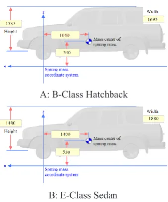
The vehicles in three categories including Hatchback and Sedan as the passenger cars, in addition to a six-axle truck with 18340 kg loading (as a heavy vehicle) are considered. The main difference between Hatchback and Sedan is in expanding rear part of the vehicle, which causes a difference in their mass center position and suspension. In Figure. 4, the characteristics of passenger cars used in our study are shown. In addition, in Figure. 5, the characteristics of the considered heavy vehicle are provided. Simulation is performed with two prospects: with braking at the start of the loop, and without breaking. In case of braking, anti-lock braking system (ABS) is used. It is assumed that the braking process reduces the speed to 20 km/h (from 80 to 60 km/h and from 70 to 50 km/h). According to Bonneson [2] and Torbic, Donnell, Brennan, Brown, O’Laughlin, and Bauer [11], deceleration rate is considered -0.85 m/s2.
Step 4) Simulation running:
loop was considered as the side friction demand factor for
safe passing from the loop. Step 5) simulation result analysis: The simulation output data were analyzed by using regression analysis, thanks to the SPSS software package.
Figure 3. The research methodology Table 1. Simulation input parameters
Parameter Number of states Descriptions
Vehicle type 3 B-Class Hatchback (1110 kg), E-Class Sedan (1650 kg),Truck (truck cab 4455 kg, trailer 5500 kg) Elevation difference 10 +4, +5, +6, +7, +8 meters-4, -5, -6, -7, -8 meters
Design type of loop ramp 2 Three-center loop Curve-Curve-Curve (C-C-C),and Spiral-Curve-Spiral (S-C-S)
Super-elevation 5 4%, 6%, 8%, 10%, 12%
Truck carries payload 1 18340 kg
Velocity 4 80 to 60 km/h and 70 to 50 km/h (for braking condition)50 and 60 km/h (for no-braking condition)
Figure 4. Passenger cars used in the simulation (values in millimeters)
A: B-Class Hatchback
B: E-Class Sedan
A: Truck cab
B: Trailer
4- Simulation results and their analysis
In this study, simulation is performed for 800 various states in CarSim and 400 various states in TruckSim, by changing the input parameters. Some of the simulation results are presented as follows:
4- 1- The effect of different parameters on the side friction demand factor for passenger cars
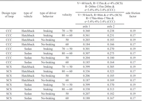
The simulation outputs for passenger cars in elevation difference of 8 meters in uphill condition are shown in Table 2. Note that in this uphill case, the second interconnecting road is 8 meters higher than first one.
According to Table 2 and other similar simulation data, the following results are attainable:
• For a safe vehicle motion on the loop, the values of friction factor assumed by AASHTO Green book are not adequate. For all simulation cases, those recommended values are less than the required friction factor derived from simulation.
• The friction factor required in front axle of the passenger cars (both Hatchback and Sedan) is more than the corresponding value in the rear axle.
• The braking condition leads to increase in the side friction demand factor, compared with the no-braking condition. This increase is in range of 73% to 136%.
• Design type of the loops is considered as one of the most important parameters, which affects the side friction demand factor.
4- 2- The effect of different parameters on the friction demand factor for heavy vehicles
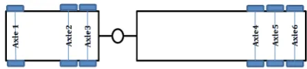
The truck employed in our simulation tests consists of 6six axles. A scheme of the truck and position of its axles are illustrated in the Figure. 6. .
As shown in Figure. 6, axles 2 and 3 are considered complementary to each other, due to their close locations (couple axles). Additionally, axles 4, 5 and 6 are coupled. The simulation outputs for heavy vehicles in elevation difference of 8 meters in uphill condition are shown in Table 3. Regarding Table 3 and other similar simulation data for heavy vehicles, the following results are achieved:
• The friction demand factor of trucks derived from the simulation is considerably greater than the one assumed by AASHTO.
• In no-braking condition, between couple axles, the maximum share of the side friction demand factor is associated to the rear axle (e.g. axle 3 in couple axles 2, 3, and axle 6 in couple axles 4, 5, 6).
Table 2. Side Friction demand Factor for trucks on upgrade*
Design type
of loop vehicletype of type of driver behavior velocity
V= 60 km/h, R=135m & e=4% (SCS) R=260m-135m-260m & e=3.4%-4%-3.4% (CCC)
side friction factor V= 50 km/h, R=86m & e=4% (SCS)
R=170m-86m-170m & e=3.4%-4%-3.4% (CCC)
axle 1 axle 2
CCC Hatchback braking 70 → 50 0.360 0.238 0.19
CCC Hatchback braking 80 → 60 0.361 0.231 0.17
CCC Hatchback No-braking 50 0.203 0.183 0.19
CCC Hatchback No-braking 60 0.184 0.166 0.17
CCC Sedan braking 70 → 50 0.301 0.270 0.19
CCC Sedan braking 80 → 60 0.307 0.275 0.17
CCC Sedan No-braking 50 0.204 0.180 0.19
CCC Sedan No-braking 60 0.185 0.164 0.17
SCS Hatchback braking 70 → 50 0.399 0.385 0.19
SCS Hatchback braking 80 → 60 0.336 0.323 0.17
SCS Hatchback No-braking 50 0.206 0.185 0.19
SCS Hatchback No-braking 60 0.187 0.169 0.17
SCS Sedan braking 70 → 50 0.399 0.370 0.19
SCS Sedan braking 80 → 60 0.338 0.313 0.17
SCS Sedan No-braking 50 0.207 0.182 0.19
SCS Sedan No-braking 60 0.188 0.167 0.17
4- 3- The comparison between passenger cars and heavy vehicles’ friction demand factor
Table 4 shows the maximum friction demand factor, for the vehicles moved in the certain height of 8 meters. To sustain the vehicle, all axles should be balanced. Balance conditions of the vehicle will be violated if at least one axle slides. Therefore, in passenger cars, the axle with the maximum friction factor is considered as the critical axle. For a truck, as a heavy vehicle, the sliding of the front axle can unbalance the truck. In addition, as shown in Figure. 6, axles 2 and 3 interact with each other and work together with complementary (located side-by-side asset of a couple of axles). Similarly, axles 4, 5 and 6 are considered a set of coupled axles. For such a set, the axle with more friction demand factor is more probable to slide. However, vehicle skidding occurs whenever the axle with less friction demand factor slides, same as the other axles. On the other hand, the axle with less friction demand factor is counted as the critical one. Therefore, for the set of coupled axles 2 and 3, the minimum friction demand factor (e.g. min (f2, f3)) is considered as the basis for maintaining the local sustainability of the rear end of the truck. Similarly, for the set of coupled axles 4, 5 and 6, the minimum friction factor (min (f4, f5, f6)) is critical. Accordingly, the critical friction demand factor of the truck is calculated as follows:
Figure 6. Positions of axles of the truck used for simulation
Table 3. Side friction demand factor for trucks on upgrade*
Design type of loop
Type of driver
behavior velocity
V=60 km/h, R=135m & e=4% (SCS),
R=260m-135m-260m & e=3.4%-4%-3.4% (CCC) side friction factor assumed
by AASHTO V=50 km/h, R=86m & e=4% (SCS),
R=170m-86m-170m & e=3.4%-4%-3.4% (CCC)
Axle 1 Axle 2 Axle 3 Axle 4 Axle 5 Axle 6
CCC braking 70 → 50 0.497 0.626 0.649 0.592 0.567 0.556 0.19
CCC braking 80 → 60 0.506 0.656 0.670 0.655 0.645 0.623 0.17
CCC No-brak-ing 50 0.297 0.186 0.288 0.056 0.186 0.307 0.19
CCC No-brak-ing 60 0.255 0.171 0.247 0.093 0.179 0.260 0.17
SCS braking 70 → 50 0.473 0.384 0.500 0.322 0.414 0.503 0.19
SCS braking 80 → 60 0.385 0.348 0.424 0.320 0.383 0.450 0.17
SCS No-brak-ing 50 0.300 0.232 0.297 0.059 0.186 0.306 0.19
SCS No-brak-ing 60 0.256 0.176 0.252 0.097 0.184 0.267 0.17
* The difference between elevations of the two interconnecting roads of the loop is equal to 8-meters.
fCritical=max(f1,(min(f2,f3 ),min(f4,f5,f6 )) (7) Regarding Table 4 and other similar tables related to other heights, the following results can be concluded:
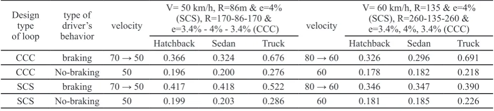
• The friction demand factors for heavy vehicles are
greater than the ones for passenger cars. This difference is in range of 27% to 52% for no-braking condition and in range of 49% to 62% for braking condition.
• Curve type is one of the effective parameters on the value of the friction demand factor.
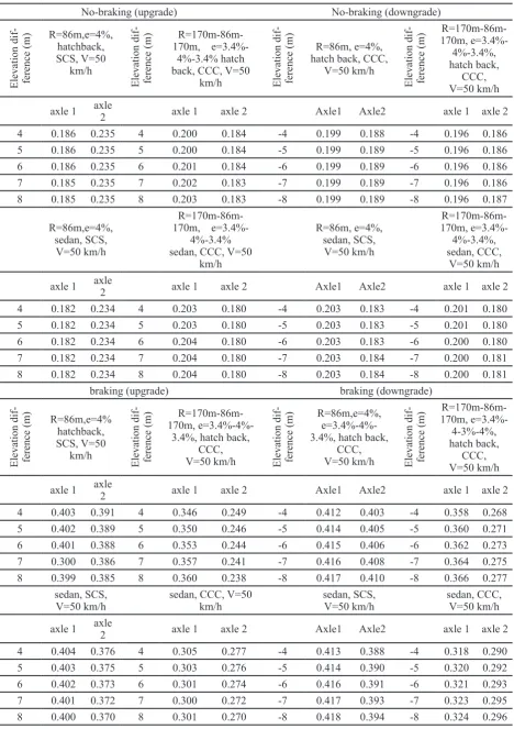
4- 4- The effect of height changes on friction demand
In Table 5, the friction demand factors associated with the passenger cars in uphill and downhill are addressed. Regarding Table 5 and other similar tables related to other heights, the following results can be concluded:
• While moving the passenger cars in uphill with constant speed, the greater the difference between elevations of the two interconnecting roads of the loop, the more side friction required to keep sustainability.
• For both types of the passenger cars, the friction demand factors differ in uphill and downhill conditions.
• In braking condition, the vehicle motion in downhill, needs more friction demand in the range of 0.1% to 6.4%, compared with uphill; whereas in no-braking condition, vehicle motion in downhill needs less friction demand in a range of 1.6% to 11.1%, compared with uphill.
4- 5- The comparison of friction demand values: AASHTO and simulation results
Table 4.: Effects of vehicle type on side friction demand factor*
Design type of loop
type of driver’s
behavior velocity
V= 50 km/h, R=86m & e=4% (SCS), R=170-86-170 &
e=3.4% - 4% - 3.4% (CCC) velocity
V= 60 km/h, R=135 & e=4% (SCS), R=260-135-260 & e=3.4%, 4%, 3.4% (CCC)
Hatchback Sedan Truck Hatchback Sedan Truck
CCC braking 70 → 50 0.366 0.324 0.676 80 → 60 0.326 0.296 0.691
CCC No-braking 50 0.196 0.200 0.276 60 0.178 0.182 0.218
SCS braking 70 → 50 0.417 0.418 0.522 80 → 60 0.346 0.347 0.390
SCS No-braking 50 0.199 0.203 0.286 60 0.181 0.185 0.226
* The difference between elevations of the two interconnecting roads of the loop is equal to -8 meters.
Downgrade, No-braking Downgrade, braking
Upgrade, braking Upgrade, No-braking
No-braking (upgrade) No-braking (downgrade)
Elevation dif
-ference (m)
R=86m,e=4%, hatchback, SCS, V=50
km/h
Elevation dif
-ference (m)
R=170m-86m-170m,
e=3.4%-4%-3.4% hatch back, CCC, V=50
km/h Elevation dif
-ference (m)
R=86m, e=4%, hatch back, CCC,
V=50 km/h
Elevation dif
-ference (m)
R=170m-86m-170m, e=3.4%-4%-3.4%, hatch back,
CCC, V=50 km/h
axle 1 axle 2 axle 1 axle 2 Axle1 Axle2 axle 1 axle 2
4 0.186 0.235 4 0.200 0.184 -4 0.199 0.188 -4 0.196 0.186
5 0.186 0.235 5 0.200 0.184 -5 0.199 0.189 -5 0.196 0.186
6 0.186 0.235 6 0.201 0.184 -6 0.199 0.189 -6 0.196 0.186
7 0.185 0.235 7 0.202 0.183 -7 0.199 0.189 -7 0.196 0.186
8 0.185 0.235 8 0.203 0.183 -8 0.199 0.189 -8 0.196 0.187
R=86m,e=4%, sedan, SCS, V=50 km/h
R=170m-86m-170m,
e=3.4%-4%-3.4% sedan, CCC, V=50
km/h
R=86m, e=4%, sedan, SCS,
V=50 km/h
R=170m-86m-170m, e=3.4%-4%-3.4%, sedan, CCC,
V=50 km/h
axle 1 axle 2 axle 1 axle 2 Axle1 Axle2 axle 1 axle 2
4 0.182 0.234 4 0.203 0.180 -4 0.203 0.183 -4 0.201 0.180
5 0.182 0.234 5 0.203 0.180 -5 0.203 0.183 -5 0.201 0.180
6 0.182 0.234 6 0.204 0.180 -6 0.203 0.183 -6 0.200 0.180
7 0.182 0.234 7 0.204 0.180 -7 0.203 0.184 -7 0.200 0.181
8 0.182 0.234 8 0.204 0.180 -8 0.203 0.184 -8 0.200 0.181
braking (upgrade) braking (downgrade)
Elevation dif
-ference (m)
R=86m,e=4% hatchback, SCS, V=50
km/h
Elevation dif
-ference (m)
R=170m-86m-170m,
e=3.4%-4%-3.4%, hatch back, CCC,
V=50 km/h Elevation dif
-ference (m)
R=86m,e=4%, e=3.4%-4%-3.4%, hatch back,
CCC,
V=50 km/h Elevation dif
-ference (m)
R=170m-86m-170m,
e=3.4%-4-3%-4%, hatch back,
CCC, V=50 km/h
axle 1 axle 2 axle 1 axle 2 Axle1 Axle2 axle 1 axle 2
4 0.403 0.391 4 0.346 0.249 -4 0.412 0.403 -4 0.358 0.268
5 0.402 0.389 5 0.350 0.246 -5 0.414 0.405 -5 0.360 0.271
6 0.401 0.388 6 0.353 0.244 -6 0.415 0.406 -6 0.362 0.273
7 0.300 0.386 7 0.357 0.241 -7 0.416 0.408 -7 0.364 0.275
8 0.399 0.385 8 0.360 0.238 -8 0.417 0.410 -8 0.366 0.277
sedan, SCS,
V=50 km/h sedan, CCC, V=50 km/h sedan, SCS, V=50 km/h sedan, CCC, V=50 km/h
axle 1 axle 2 axle 1 axle 2 Axle1 Axle2 axle 1 axle 2
4 0.404 0.376 4 0.305 0.277 -4 0.413 0.388 -4 0.318 0.290
5 0.403 0.375 5 0.303 0.276 -5 0.414 0.390 -5 0.320 0.292
6 0.402 0.373 6 0.301 0.274 -6 0.416 0.391 -6 0.321 0.293
7 0.401 0.372 7 0.300 0.272 -7 0.417 0.393 -7 0.323 0.295
8 0.400 0.370 8 0.301 0.270 -8 0.418 0.394 -8 0.324 0.296
Table 6. Difference between side friction demand factors resulting from the simulations and the recommended values of AASHTO
vehicle type Grade No-braking braking
50 km/h 60 km/h 50 km/h 60 km/h
Sedan
all grades 5.9% 7.5% 91.9% 89.6%
upgrade 6.9% 8.2% 85.6% 88.5%
downgrade 4.9% 6.5% 98.2% 90.6%
Hatch back
all grades 4.1% 5.9% 102.7% 101.2%
upgrade 5.7% 7.1% 97.4% 104.1%
downgrade 2.5% 4.1% 107.6% 98.4%
Truck
all grades 54.4% 41.8% 194.6% 212.5%
upgrade 61.3% 50.2% 188.4% 210.4%
downgrade 47.4% 33.5% 200.8% 214.7%
Passenger cars
all grades 5.0% 6.5% 97.3% 95.4%
upgrade 6.3% 7.6% 91.8% 96.4%
downgrade 3.7% 5.4% 102.9% 94.5%
All vehicles
all grades 21.5% 18.3% 129.7% 134.5%
upgrade 24.6% 21.8% 124.0% 134.4%
downgrade 18.3% 14.8% 135.5% 134.6%
5- Regression analysis
As shown in the previous section, the change in simulation input parameters cancould substantially change the friction demand factor. It was also observed that in some circumstances, the AASHTO assumed values for the friction demand factor are less than the required ones. Therefore, in the present study, we attempt to provide the practical models by using regression analysis, in order to determine the friction demand factor. The simulator inputs are considered as model parameters. In order to analyze the data, SPSS 24 is used. Data analysis is performed based on five different categories of the vehicles: Hatchback, Sedan, heavy vehicle (truck), passenger vehicles, and all three types of the vehicles. In the process of doing the analysis, first-step correlation analysis has been done to explore the variables correlated with the demand friction factor and due to the fact that all the independent variables should be independent. At second-step, the variables correlated with the demand friction factor were candidates to enter the equation as independent variables (according to this point of view, all the independent variables should be independent; table Table 7 is an example of correlation analysis). At third-step, by regression analysis the data were analyzed. In the process of regression analysis, the variables correlated with the demand friction factor were entered into the equation as independent variables, then the significant variables were maintained in the model and the other variables were deleted from the model by the trial and error method. At last, the model that had the maximum numerical R-squared index (R2) was selected as the best model. In these models, the axle’s friction demand factor is considered as the dependent variable. All variables used in regression analysis are explained in Table 8. In Table 8, the value fAASHTO comes from Figure. 2. Since in this study, the value Rmin is calculated based on the AASHTO assumed
values, the value fAASHTO can also be calculated via Eq. 8: (8) The regression models are conducted for each of the mentioned five categories. For example, the results of regression analysis for Hatchback category are provided in Table 9.
In Table 9, if the error of a parameter is less than 0.05 (i.e. index t is more than 1.96), that parameter enters the regression model. The parameter coefficients are also provided in column B. The friction demand models obtained from regression analysis are provided as follows (statistical tests or judgments are provided in Table 9 to table 15Table 15):
Hatchback’s front axle: fdemand=-0.096+V2/(78.01R
min)-1.628emax-0.016 LT+0.003 Elv-0.011g+0.206|ba | (9) Hatchback’s rear axle:
fdemand=V2/(112.49Rmin)-1.129emax-0.055LT-0.004 Elv-0.005g+0.02|g|+0.162|ba |
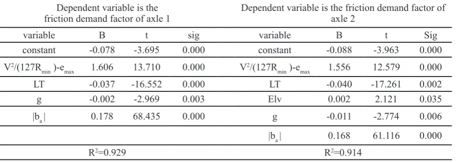
(10) Sedans’ front axle:
fdemand=-0.078+V2/(79.08R
min)-1.606emax-0.037 LT-0.002g+0.178|ba | (11) Sedans’ rear axle:
fdemand=-0.088+V2/(81.15R
min)-1.565emax-0.04 LT+0.002 Elv-0.011g+0.168|ba | (12)
2
max min 127 AASHTO V
f e
R
Passenger cars’ front axle:
fdemand=-0.065+V2/(78.54Rmin)-1.617emax-1.565×10-5 (m)-0.026 LT+0.002 Elv-0.01g+0.192|ba |
(13) Passenger cars’ rear axle:
fdemand=-0.099+V2/(77.16Rmin)-1.646emax -0.048LT-0.004g+0.165|ba |
(14) First trucks’ axle:
fdemand=V2/(99.14R
min)-1.281emax+0.043LT+0.003 Elv-0.008 |Elv|-0.012g+0.048|g|+0.248|ba | (15) Second trucks’ axle:
fd e m a n d= V2/ ( 2 2 4 . 7 8 Rm i n) - 0 . 5 6 5 em a x+ 0 . 1 2 9 LT+0.413|ba |
(16) Third trucks’ axle:
fdemand=V2/(111.60R
min)-1.138emax
+0.088LT-0.004g+0.023|g|+0.342|ba | (17)
Fourth trucks’ axle: fdemand=-V2/(1165.18R
min)+0.109emax+0.167
LT+0.49|ba | (18)
Fifth trucks’ axle:
fd e m a n d= V2/ ( 1 8 2 . 7 3 Rm i n) - 0 . 6 9 5 em a x+ 0 . 11 9 LT+0.385|ba |
(19) Sixth trucks’ axle:
fdemand=V2/(85.35Rmin)-1.488emax+0.069 LT+0.293|ba| (20) Required friction demand factor to maintain stability of passenger cars:
fdemand=V2/(103.34Rmin)-1.229emax-1.783× 10-5(m)-0.026 LT+0.006|g|+0.192|b
a |
(21) Required friction demand factor to maintain stability of truck:
fd e m a n d= V2/ ( 1 2 2 . 9 4 R
m i n) - 1 . 0 3 3 em a x+ 0 . 1 0 7
LT+0.022|g|+0.327|ba | (22)
Required friction demand factor to maintain stability of all types of vehicles:
fdemand=V2/(276.69Rmin)-0.459emax+4.192 ×10-5(m)+0.018 LT+0.019|g|+0.236|b
a |
(23)
Table 7. Correlation analysis to maintain stability of all types of vehicles (SPSS outputs)
fAASHTO m LT |g| |ba |
fAASHTO
Pearson Correlation 1 .000 .000 .605** .000
Sig. (2-tailed) 1.000 1.000 .000 1.000
N 1200 1200 1200 1200 1200
m
Pearson Correlation .000 1 .000 .000 .000
Sig. (2-tailed) 1.000 1.000 1.000 1.000
N 1200 1200 1200 1200 1200
LT
Pearson Correlation .000 .000 1 -.057* .000
Sig. (2-tailed) 1.000 1.000 .047 1.000
N 1200 1200 1200 1200 1200
|g|
Pearson Correlation .605** .000 -.057* 1 .000
Sig. (2-tailed) .000 1.000 .047 1.000
N 1200 1200 1200 1200 1200
|ba |
Pearson Correlation .000 .000 .000 .000 1
Sig. (2-tailed) 1.000 1.000 1.000 1.000
N 1200 1200 1200 1200 1200
Table 8. Variables used in regression analysis
Variable description
fdemand Side friction demand factor for safe passing through loop fAASHTO Side friction demand factor recommended by AASHTO
LT 1 if loop type is C-C-C, and 0 if S-C-S
Elv Difference between elevations of two interconnecting roads of loop
g Slope of the loop
ba Brake deceleration rate
m Mass of the vehicle
V Design speed of the loop
Rmin Minimum radius of the loop
emax Maximum super-elevation of the loop
Table 9. Results of Statistical Analysis for Hatchback vehicle by SPSS Software
Dependent variable is the
friction demand factor of axle 1 Dependent variable is the friction demand factor of axle 2
variable B t sig variable B t Sig
constant -0.096 -6.630 0.000 V2/(127R
min )-emax 1.129 28.768 0.000 V2/(127R
min )-emax 1.628 20.329 0.000 LT -0.055 -17.552 0.000
LT -0.016 -10.412 0.000 Elv -0.004 -3.167 0.002
Elv 0.003 4.629 0.000 g -0.005 -4.580 0.000
g -0.011 -4.625 0.000 |g| 0.020 3.888 0.000
|ba | 0.206 115.605 0.000 |ba | 0.162 44.629 0.000
R2=0.972 R2=0.985
Table 10. Results of Statistical Analysis for Sedan vehicle by SPSS Software
Dependent variable is the
friction demand factor of axle 1 Dependent variable is the friction demand factor of axle 2
variable B t sig variable B t Sig
constant -0.078 -3.695 0.000 constant -0.088 -3.963 0.000
V2/(127R
min )-emax 1.606 13.710 0.000 V2/(127Rmin )-emax 1.556 12.579 0.000
LT -0.037 -16.552 0.000 LT -0.040 -17.261 0.002
g -0.002 -2.969 0.003 Elv 0.002 2.121 0.035
|ba | 0.178 68.435 0.000 g -0.011 -2.774 0.006
|ba | 0.168 61.116 0.000
Table 11. Results of Statistical Analysis for Passenger cars vehicle by SPSS Software
Dependent variable is the
friction demand factor of axle 1 friction demand factor of axle 2Dependent variable is the
variable B t sig variable B t Sig
constant -0.065 -4.555 0.000 constant -0.099 -5.276 0.000
V2/(127R
min )-emax 1.617 21.071 0.000 V2/(127Rmin )-emax 1.646 15.871 0.000
m -1.568E-5 -5.837 0.000 LT -0.048 -24.448 0.000
LT -0.026 -18.065 0.000 g -0.004 -5.510 0.000
ELV 0.002 3.838 0.000 |ba | 0.165 71.569 0.000
g -0.010 -4.301 0.000
|ba | 0.192 112.549 0.000
R2=0.944 R2=0.914
Table 12. Results of Statistical Analysis for each of Trucks’ axles by SPSS Software
Dependent variable is the
friction demand factor of axle 1 friction demand factor of axle 2Dependent variable is the
variable B t sig variable B t Sig
constant 1.281 33.111 0.000 V2/(127R
min )-emax 0.565 16.002 0.000 V2/(127R
min )-emax 0.043 14.015 0.000 LT 0.129 17.560 0.000
LT 0.003 2.401 0.017 |ba | 0.413 47.794 0.000
ELV -0.008 -5.711 0.000
|ELV| -0.012 -2.408 0.017
g 0.048 9.471 0.000
|g| 0.248 69.399 0.000
|ba | 1.281 33.111 0.000
R2=0.994 R2=0.966
Dependent variable is the
friction demand factor of axle 3 friction demand factor of axle 4Dependent variable is the V2/(127R
min )-emax 1.138 21.003 0.000 V2/(127Rmin )-emax -0.109 -2.577 0.010
LT 0.088 17.422 0.000 LT 0.167 18.971 0.000
g -0.004 -2.128 0.034 |ba | 0.490 47.377 0.000
|g| 0.023 3.706 0.000
|ba | 0.342 57.884 0.000
R2=0.988 R2=0.943
Dependent variable is the
friction demand factor of axle 5 friction demand factor of axle 6Dependent variable is the V2/(127R
min )-emax 0.695 22.067 0.000 V2/(127Rmin )-emax 1.488 64.962 0.000
LT 0.119 18.220 0.000 LT 0.069 14.385 0.000
|ba | 0.385 49.926 0.000 |ba | 0.293 52.268 0.000
Table 13. Results of Statistical Analysis for maintain stability of passenger cars by SPSS Software
Dependent variable
variable B t sig
V2/(127R
min )-emax 1.229 45.095 0.000
m -1.783E-5 -6.691 0.000
LT -0.026 -17.646 0.000
|g| 0.006 3.034 0.002
|ba | 0.192 110.42 0.000
R2=0.995
Table 14. Results of Statistical Analysis for maintain stability of truck by SPSS Software
Dependent variable
variable B t sig
V2/(127R
min )-emax 1.033 15.664 0.000
LT 0.107 17.454 0.000
|g| 0.022 2.832 0.005
|ba | 0.327 45.475 0.000
R2=0.981
Table 15. Results of Statistical Analysis for maintain stability of all types of vehicles by SPSS Software
Dependent variable
variable B t sig
V2/(127R
min )-emax 0.459 11.348 0.000
m 4.192E-5 36.138 0.000
LT 0.018 5.300 0.000
|g| 0.019 4.322 0.000
|ba | 0.236 58.929 0.000
R2=0.971
In Equations 9 to 14, the friction demand factor of each front and rear axles (dependent variables) of the passenger cars are examined separately. In Equations 13 and 14, the friction demand factor of each rear and front axle of the passenger cars are checked by combining the Sedan and Hatchback data. In Equations 15 to 20, the friction demand (dependent variable) of each of six axles of truck is examined separately. Here, the vehicle sustainability is defined as passing from the loop ramp without deviation from its route. On the other hand, in case of one axle skidding, the complete body of the vehicle goes unbalanced. In Equations 21 to 23, all the vehicle axles should be balanced in order to maintain sustainability of the vehicle. In Equation 21, it is assumed that the axle which needs more friction demand factor is considered as the critical one, from vehicle skidding point of
view. Then this axle can cause vehicle deviation. Therefore, to acquire Equation 21, the axle with more friction demand factor is regarded as the one for which the dependent variable is calculated. Equation 22 is related to the truck in the friction demand factor model. In the procedure of finding this model, the assumptions mentioned to calculate the minimum friction factor based on sets of coupled axles are respected. Finally, in Equation 23, the friction demand model associated with the data of all vehicles (passenger and heavy vehicles) is provided.
6- Conclusions
The aim of this study is to evaluate the friction demand factor in loop ramp. This type of turning roadway facilities is commonly used in interchanges. The substantial exclusivity of these types of the ramps is the existence of the horizontal curves, combined with the longitudinal grades. In the proposed methodology of this paper, the CarSim and TruckSim software packages are employed, as the simulation tools. They are able to animate the vehicle performance and plot the diagrams. Several parameters are considered as the inputs of the simulation. The vehicles used in simulations are Hatchback and Sedan (as passenger cars) and Truck (as heavy vehicle). Simulation is performed for two various types of loops, including Curve-Curve-Curve (C-C-C) and Spiral-Curve-Spiral (S-C-S), in two different conditions (braking, and no-braking). The results of the study show that the friction demand values recommended by AASHTO (as geometric design guideline) are uncertain. In other words, to ensure safe vehicle passing from loops, the assumed friction factors by AASHTO are lower than the required friction factor (derived from simulation). For no-braking condition, these differences in uphill and downhill states are 24% and 18%, respectively. For braking condition, the difference between simulation results and the AASHTO values, in uphill and downhill are 124% and 135%, respectively. The main reason of these considerable differences may be the type of the models used in AASHTO and the simulation process. In the AASHTO guideline, the Point Mass (PM) model is used for the friction demand calculation. In the PM model, parameters related to the vehicle, curve type, elevation difference, uphill/ downhill states in moving directions, braking deceleration, etc. are ignored. While, in our study, simulation is performed based on a multi-body model, and all mentioned parameters are considered in the simulation process. According to other results, friction factor required in front axle of passenger cars is more than the corresponding value in their rear axle. In addition, the simulation verified the fact that the braking condition results in the increase of the friction demand factor. This increase is in the range of 73% to 136% (compared to the condition of no-braking). Furthermore, heavy vehicles’ friction demand is more than the one related to passenger cars. This difference is in the range of 27% to 52% for the condition of no-braking and in the range of 49% to 62% for the condition of braking. Based on the regression analysis of the simulation results, the friction demand factor models are achieved for different conditions. The findings of the study verify the necessity of the revising friction demand values, especially for the design of interchange loop ramps.
References
Please cite this article using:
M. H. Dehshiri Parizi, M. Tamannaei, H. Haghshenas, The evaluation of the Friction Demand Factor in Loop Ramps
of Interchange Facilities, AUT J. Civil Eng., 2(2) (2018) 195-208.
DOI: 10.22060/ajce.2018.14330.5472
crashes and tire–pavement friction: a case study, International Journal of Pavement Engineering, 18(2) (2017) 119-127.
[2] A. Mehrara Molan, A. Abdi Kordani, Multi-Body Simulation Modeling of Vehicle Skidding and Roll over for Horizontal Curves on Longitudinal Grades, in: Transportation Research Board 93rd Annual Meeting, 2014.
[3] A.A. Kordani, A.M. Molan, The effect of combined horizontal curve and longitudinal grade on side friction factors, KSCE Journal of Civil Engineering, 19(1) (2015) 303-310.
[4] A.A.o.S. Highway, T. Officials, A Policy on Geometric Design of Highways and Streets, 2011, Aashto, 2011. [5] S.M. Easa, E. Dabbour, Design radius requirements
for simple horizontal curves on three-dimensional alignments, Canadian Journal of Civil Engineering, 30(6) (2003) 1022-1033.
[6] E. Donnell, J. Wood, S. Himes, D. Torbic, Use of Side Friction in Horizontal Curve Design: A Margin of Safety Assessment, Transportation Research Record: Journal of the Transportation Research Board, (2588) (2016) 61-70. [7] T. Varunjikar, Design of horizontal curves with
downgrades using low-order vehicle dynamics models, The Pennsylvania State University, 2011.
[8] S. Mavromatis, B. Psarianos, P. Tsekos, G. Kleioutis, E. Katsanos, Investigation of vehicle motion on sharp horizontal curves combined with steep longitudinal grades, Transportation Letters, 8(4) (2016) 220-228. [9] T.-H. Chang, Effect of vehicles’ suspension on highway
horizontal curve design, Journal of transportation engineering, 127(1) (2001) 89-91.
[10] D. Torbic, M. O’Laughlin, D. Harwood, K. Bauer, C. Bokenkroger, L. Lucas, J. Ronchetto, S. Brennan, E. Donnell, A. Brown, NCHRP Report 774: Superelevation Criteria for Sharp Horizontal Curves on Steep Grades, Transportation Research Board of the National Academies, Washington, DC, (2014).
[11] D. Torbic, E. Donnell, S. Brennan, A. Brown, M. O’Laughlin, K. Bauer, Superelevation design for sharp horizontal curves on steep grades, Transportation Research Record: Journal of the Transportation Research Board, (2436) (2014) 81-91.
[12] F. Awadallah, Theoretical analysis for horizontal curves based on actual discomfort speed, Journal of transportation engineering, 131(11) (2005) 843-850. [13] J. Hall, K. Smith, L. Titus-Glover, J. Wambold, T. Yager,
Z. Rado, Guide for pavement friction. NCHRP. Web-only document 108. Contractor’s inal Report NCHRP Project 01-43, Transportation Research Board of the National Academes, (2009).
[14] J. Morrall, R. Talarico, Side friction demanded and margins of safety on horizontal curves, Transportation Research Record, 1435 (1994) 145.
[15] http://www.carsim.com, Mechanical Simulation Corporation, in, 2017.
[16] G. Furtado, S. Easa, A. Abd El Halim, Vehicle stability on combined horizontal and vertical alignments, National Library of Canada= Bibliothèque nationale du Canada, 2003.
[17] M.W. Sayers, Vehicle dynamics programs for roadway and roadside studies, UMTRI-98-20-1, Transportation Research Institute, University of Michigan, 1999.
[18] A.A. Kordani, A.M. Molan, S. Monajjem, New Formulas of Side Friction Factor Based on Three-Dimensional Model in Horizontal Curves for Various Vehicles, in: T&DI Congress 2014: Planes, Trains, and Automobiles, 2014, pp. 592-601.
[19] A.A. Kordani, M.H. Sabbaghian, B. Tavassoli Kallebasti, Analyzing the influence of Coinciding Horizontal Curves and Vertical Sag Curves on Side Friction Factor and Lateral Acceleration Using Simulation Modeling, TRR Journal, (2015).
[20] J. Bonneson, NCHRP Report 439: Superelevation Distribution Methods and Transition Designs, Transportation Research Board, National Research Council, Washington, DC, (2000).
[21] J.A. Bonneson, Side friction and speed as controls for horizontal curve design, Journal of Transportation engineering, 125(6) (1999) 473-480.
[22] S. Easa, A. El Halim, Radius requirements for trucks on three-dimensional reverse horizontal curves with intermediate tangents, Transportation Research Record: Journal of the Transportation Research Board, (1961) (2006) 83-93.
[23] J. Gattis, B. Finley Vinson III, L.K. Duncan, Low-speed horizontal curve friction factors, Journal of transportation engineering, 131(2) (2005) 112-119.
[24] S. Mavromatis, E. Papadimitriou, B. Psarianos, G. Yannis, Vehicle Skidding Assessment through Maximum-Attainable Constant-Speed Investigation, Journal of Transportation Engineering, Part A: Systems, 143(9) (2017) 04017044.
[25] H.F. Mollashahi, K. Khajavi, A.K. Ghaeini, Safety Evaluation and Adjustment of Superelevation Design Guides for Horizontal Curves Based on Reliability Analysis, Journal of Transportation Engineering, Part A: Systems, 143(6) (2017) 04017013.