A three-dimensional numerical model to estimate the fall velocity of
sediment particles
Mohsen Monadi , Hamed Taghizadeh, Mirali Mohammadi
Department of Civil Engineering, School of Water and Hydraulic Structures Engineering, Urmia University, Urmia, Iran
Date of submission: 18 Oct 2017, Date of acceptance: 02 Mar 2019
ABSTRACT
The fall velocity of sediment particles plays a key role in sediment transport studies. Researchers have attempted to determine the terminal fall velocity, and most of the studies in this regard have been based on experimental, quasi-experimental, and in-situ measurements. The present study aimed to use a numerical model to estimate the fall velocity of a single sediment particle in distilled and motionless water. We used spherical quartz particles with the diameters of 0.77, 1.09, 2.18, and 4.36 millimeters and density of 2,650 kg/m3. The Flow-3D software was applied to estimate the fall velocity based on the environment of experiment by Ferguson and Church (2004) using the void of flow method. The main objective of this research was to demonstrate the power of the numerical model to simulate the fall velocity of sediment particles. To validate the results of the model, they were compared with the experimental results and 26 well-known publications during 1933-2016 using the root-square-mean and mean-absolute-percentage errors. The results showed good agreement between the experimental and numerical data. Therefore, the proposed numerical model could be used to determine the fall velocity of sediment particles with a wide range of diameters in the proposed environment and particle types.
Keywords:Fall velocity, Sediment particle, Flow-3D, Void of flow, Distilled water
Introduction
Study of sediment transport in river engineering problems requires an appropriate equation to predict the terminal settling velocity of the sediment particles with high accuracy; such problems include sedimentation in river directions, designing settling basins of water transmission branches, morphological alteration of river banks, and sedimentation of dam reservoirs. Errors in the prediction of the settling velocity may increase by a factor of three or more in the computation of the suspended load transport. For a single particle, the fall velocity (ws) could be determined based on the
equilibrium between gravity, buoyancy, and drag forces. Settling velocity mainly depends on the density, size, and shape of the sediment particles.
Mohsen Monadi
Citation: Monadi M, Taghizadeh H, Mohammadi M. A three-dimensional numerical model to estimate the fall velocity of
Several studies have been conducted to determine particle fall velocity. The first study in this regard was performed by Stokes (1851; cited in Graf,1 followed by Rouse,2 and Corey.3 Fair and Geyer presented an equation based on fall velocity and particle diameter, which had to be solved through trial and error.4 In another research, Zanke presented a formula based on viscosity, particle density, and diameter to calculate the fall velocity of sediment particles.5 In addition, Yalin presented an equation based on the combination of effective diameter and particle Reynolds number,6 and Hallermier presented three equations with different settling regimes for quartz in water.7
dimensionless terminal velocity in terms of dimensionless particle diameter.10 Furthermore, Van Rijn proposed three formulas for three ranges of particle diameters,11 while Concharov presented two equations for two ranges of particle diameters (cited in Ibad-Zadeh).12
Julien proposed an equation to calculate fall velocity based on the diameter and density of sediment particles and water viscosity,13 and Cheng developed a formula to calculate the fall velocity of natural sediment particles, which is applicable to a wide range of Reynolds numbers.14 In addition, Ahrens claimed that the Archimedes buoyancy index is the fundamental independent variable for Reynolds number fall velocity and the normalized sediment scale parameter, proposing an equation that could be used over a wide range of conditions.15, 16 Similarly, Jimenez and Madsen presented a formula to estimate natural sediment particles in the grain sizes of 0.063-1 millimeter.17
Brown and Lawler proposed two new correlations of sphere terminal velocity for two ranges of Reynolds numbers (>2×10⁵ and >4,000),18 while Ferguson and Church presented a new equation for sediment fall velocity as a function of particle diameter.19 Moreover, She et al. derived an equation to denote a correlation between particle size and particle fall velocity in natural sediment particles using video imaging technique,20 and Camenen proposed a general formula based on the shape and roundness of the particles, which could be applied to any particle.21
Sadat-Helbar et al. developed a fuzzy regression concept to estimate the fall velocity of natural sediment particles,22 while Wu and Wang examined several formulas for initial porosity and fall velocity.23 In another study in this regard, Monadi et al. compared several equations for the calculation of fall velocity, proposing a new formula using the regression method.24 On the other hand, Chang and Liou proposed a formula to calculate the settling velocity of non-cohesive sediments,25 which is similar to the findings of Rubey26 and Souleby.27
To date, no studies have been focused on the 3D simulation of this phenomenon using a numerical model, such as the flow-3D software.
Although several studies have predicted settling velocity, they have been faced with limitation in its application in river engineering projects. For instance, the formulas proposed by Stokes, Rouse,2 and Brown and Lawler18 are only appropriate for spherical particles. In addition, some of the aforementioned models and formulas require trial and error in order to calculate the settling velocity of a particle (e.g., Fair and Geyer). Furthermore, some of the proposed correlations are only applicable to specific domain of Reynolds number (e.g., Stokes, Khan and Richardson, and Turton and Clark). Evidently, decision-making on selecting an appropriate and optimal formula is difficult considering the variety of the solutions presented for the same problem. Therefore, an appropriate and accurate numerical model could help calculate the fall velocity of sediment particles with high accuracy through validating an optimal numerical model based on an experimental dataset and using empirical formulas.
The current research aimed to present a simple formula to estimate the fall velocity of spherical particles using a numerical model. The formula has been derived from the proposed numerical model by comparing the experimental data proposed by Ferguson and Church (2004). Additionally, the numerical results have been compared with 26 well-known correlations in the previous studies with the aim of achieving a simple formula based on the equilibrium between accuracy and simplicity and validating the proposed numerical model.
Materials and Methods
The terminal settling velocity for a particle occurs when the gravity force minus the buoyancy force equals the drag force, as follows:
Fg- Fp=Fd (1)
where Fg is the gravity force, Fp represents the
buoyancy force, and Fd shows the drag force.
and could be calculated using the following equation:
ws= 1 18
s-1 gDs2
v 2
where s shows the relative specific density (ρs/ρ), v is the kinematic viscosity of the fluid
(m2/s), Rs represents the Reynolds number
(wsDs/v), Ds is the diameter of the particle (m), ρ and ρs are the density of the fluid and particle
(kg/m3), respectively, g denotes the gravitational acceleration (9.81 m/s2), and ws is
the settling velocity (m/s).
To introduce the use of the Flow-3D software to estimate the fall velocity of the spherical sand particles with the mentioned diameters and specific density in this study, the following steps were performed:
1. Using the Flow-3D software, all the particles were modeled based on the experimental environment proposed by Ferguson and Church (2004). The features of the model setup are presented in Table 1.
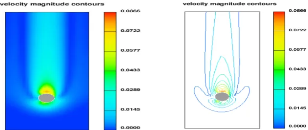
2. The fall velocity of each particle was calculated using the numerical model and void of flow (VOF) method. The results are shown in Table 2, and the velocity magnitude contours of the particles are depicted in Figures 1-4. 3. The experimental data proposed by Ferguson
and Church (2004) for the selected particles are presented in Table 3.
4. The fitness between the numerical and experimental findings and 26 well-known relations was assessed using the root-mean-square error (RMSE) and mean absolute percentage error (MAPE) based on Equations
3-4, and the results are shown in Table 4. The agreement between the two datasets is shown in Fig. 5.
RMSE ∑ni 1 Eni-Ni 2 100 3
MAPE 100n EiE-Ni
i n
i 1
4
where E and N are the experimental and numerical data, respectively, and n is the number of the data.
5. The correlation between the fall velocity and diameter of the particles is shown in Figures 6-7 for the numerical and experimental datasets.
6. The correlation between the non-dimensional fall velocity and effective diameter (Dgr) of the particles is depicted in Figures 8-9 for the numerical and experimental datasets.
Dgr D g s-1v2
1
3 5
where D is the particle diameter (m), g
represents the acceleration due to gravity (m/s2), s shows the relative density of the particles, and v is the kinematic viscosity of the fluid (m2/s).
Flow 3D software
The numerical model used to simulate the settling condition was the FLOW-3D, which is a general purpose of the CFD software for the modeling of multi-physics flow problems, heat transfer, and solidification based on the finite volume method to solve the Reynolds-averaged Navier-Stokes equations of the fluid motion in the Cartesian coordinates. For each cell, the average values of the flow parameters (pressure and velocity) were computed at discrete times using a staggered grid technique (Flow 3D, 2010).
Calibration of the computational model
The calibration and validation of the numerical models are of paramount importance. Therefore, it constitutes part of the analysis tasks in most CFD models. In fact, an ongoing effort to carry out validation against the published or experimental data remains essential, particularly to ensure modeling accuracy and provide a high confidence level in its application.
in some of the formula derived for non-spherical particles, a shape factor was used to correct the results.
All the features of the model setup were selected based on the environment and particle size range via trial and error in various numerical models. Considering the lower and
upper sizes of the particles, the interpolation process was performed more efficiently and could be expanded to the interior zone. Additionally, the selected numerical model could achieve an appropriate pattern between the lower and upper boundaries of the particle sizes among the other numerical models.
Model setup
Table 1 shows the data on the meshing and boundary conditions.
Table 1. Features of model setup
Meshing
Model Type VOF
Meshing Type Matching rectangle Number of computational blocks 1
Number of computational Volume 500000
Boundary conditions Sphere body Solid Lateral boundaries Wall
Equations
Turbulence model RNG
Algorithm to solve the pressure equation GMRES Algorithm to solve the fluid shear stress Explicit Free surface model VOF
Time interval 0.01
Geometry Settling distance of 1.0 meter in a cylinder of length 1.2 meter
Results and Discussion
The experiments in the present study were performed based on the procedures proposed by Ferguson and Church (2004), and the numerical simulations were carried out using the Flow-3D software. The numerical and experimental fall velocity magnitudes are presented in Tables 2, respectively. According to the information in these tables, the numerical results were close to the experimental results, indicating the good performance of the numerical model to simulate fall velocity. Therefore, the proposed numerical model and equations were used to determine the fall velocity of the sediment particles in this condition.
Table 2. The Numerical and experimental results of fall velocity Numerical results Experimental measurements D (mm) Ws (m/s) D (mm) Ws (m/s)
0.77 0.095 0.77 0.093
1.09 0.134 1.09 0.141
2.18 0.220 2.18 0.209
4.36 0.335 4.36 0.307
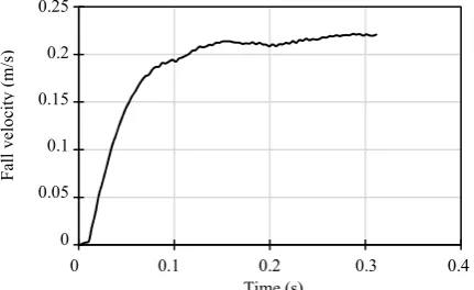
The simulated velocity fields for each particle while settling in motionless water are depicted in Figures 1-4. Accordingly, the time to achieve uniform velocity distribution differed in each particle depending on the size of the particles. The time was plotted versus fall velocity (Figures 5-8). As can be seen in these figures, the increased size of the particles was associated with the increased time to achieve uniform fall velocity.
Fig. 2. Velocity magnitude contour of particle with diameter of 1.09 mm
Fig. 3. Velocity magnitude contour of particle with diameter of 2.18 mm
Fig. 4. Velocity magnitude contour of particle with diameter of 4.36mm
Fig. 5. Velocity magnitude contour of particle with diameter of 0.77 mm
Fig. 6. Particle velocity versus time in particle with diameter of 1.09 mm
0 0/02 0/04 0/06 0/08 0/1 0/12
0 0/1 0/2 0/3 0/4
Fall
v
elocity
(m/s)
Time (s)
0 0/05 0/1 0/15 0/2 0/25
0 0/1 0/2 0/3 0/4
Fall
v
elocity
(m/s)
Time (s) 0.12
0.1 0.08 0.06 0.04 0.02 0
0.25 0.2 0.15 0.1 0.05 0
Fig. 7. Particle velocity versus time in particle with diameter of 2.18 mm
Fig. 8. Particle velocity versus time in particle with diameter of 4.36 mm
To determine the accuracy of the numerical model, the numerical and experimental results were calculated using RSME and MAPE (Table 3). According to the information in Table 3, the numerical results had good agreement with the experimental results, especially in the particles with diameters of 0.77 and 1.09 millimeters. The agreement between the numerical and experimental data is depicted in Fig. 9. Furthermore, the numerical results were compared with 26 famous proposed relations (Table 4).
Table 3. Root-Mean-Square and mean absolute percentage errors in numerical model and experimental results
Diameter (mm) RSME MAPE 0.77 0.2 2.15 1.09 0.2 1.42 2.18 1.1 5.26 4.36 2.8 9.12 Total 1.5 4.5
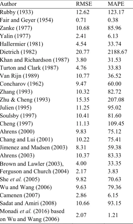
According to the information in Table 4, the relation proposed by Fair and Geyer (1954) had the best agreement with the numerical results, with the RMSE and MAPE values estimated at 0.71 and 0.38, respectively. However, this relation requires a trial-and-error solution in order to calculate the fall velocity of a particle that takes a long time and an onerous work.
Another relation in this regard has been proposed by Monadi et al. based on the relation presented by Wu and Wang, which had good agreement with the numerical results. However, it is only valid for the sediment particles with specific density (2.65) and sediment diameters within the range of 0.55-4.36 millimeters. As is
depicted in Fig. 9, the relation proposed by Ferguson and Church (2004) had good agreement with the numerical results as a universal relation. Moreover, it could be observed that the Flow-3D software could be used to calculate the fall velocity of the sediment particles with high accuracy.
Table 4. Root-Mean-Square and mean absolute percentage errors in numerical model and 26 famous relations
0 0/05 0/1 0/15 0/2 0/25
0 0/1 0/2 0/3 0/4
Fall
v
elocity
(m/s)
Time (s)
0 0/05 0/1 0/15 0/2 0/25 0/3 0/35 0/4
0 0/1 0/2 0/3 0/4
Fall
v
elocity
(m/s)
Time (s)
Author RMSE MAPE
Rubby (1933) 12.62 123.17 Fair and Geyer (1954) 0.71 0.38 Zanke (1977) 10.68 85.96 Yalin (1977) 2.41 6.13 Hallermier (1981) 4.54 33.74 Dietrich (1982) 20.77 2188.67 Khan and Richardson (1987) 3.80 31.53 Turton and Clark (1987) 4.76 33.83 Van Rijn (1989) 10.77 36.52 Concharov (1962) 9.47 60.00 Zhang (1993) 10.32 82.72 Zhu & Cheng (1993) 15.35 207.08 Julien (1995) 11.25 95.02 Soulsby (1997) 10.41 81.60 Cheng (1997) 11.13 109.45 Ahrens (2000) 9.83 75.12 Chang and Lui (2001) 10.22 75.41 Jimenez and Madsen (2003) 8.31 59.38 Ahrens (2003) 10.37 83.33 Brown and Lawler (2003), 4.00 33.35 Ferguson and Church (2004) 2.17 3.83 She et al. (2005) 9.82 70.63 Wu and Wang (2006) 9.63 79.36 Camenen (2007) 2.86 6.15 Sadat and Amiri (2008) 10.66 93.15 Monadi et al. (2016) based
on Wu and Wang (2006) 2.07 1.21 0 0.1 0.2 0.3 0.4
0.4 0.35 0.25 0.2 0.15 0.1 0.05 0
0 0.1 0.2 0.3 0.4 0.25
Fig. 9. Agreement between experimental data of ferguson and Church (2004) and numerical data
In order to develop a new and simple correlation, the fall velocity of each particle was plotted versus the diameter of the particle for the numerical data (Fig. 10). In addition, a curve fitting was used to determine the correlation between fall velocity and particle diameter (R2=0.9922).
Fig. 10. Correlation of fall velocity and diameter in numerical data
10
ws=0.1357ln D +0.12
R2=0.9922
In another attempt, we used the non-dimensional effective diameter (Dgr) and fall
velocity (w’
s) instead of the diameter and
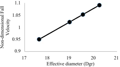
velocity of the particles so as to improve Equation 10. The results are shown in Fig. 11.
Fig. 11. Correlation between non-dimensional fall velocity and effective diameter in numerical data
' (11)
ws=0.0539Dgr
R²=1
Conclusion
Several researchers have proposed the correlations between fall velocity (ws) and particle diameter (D) experimentally and theoretically. In the present study, we derived a simple formula using the setup of a numerical model for quartz particles in motionless, pure water at the temperature of 23-24 oC in the grain sizes within the diameter range of 0.77-4.36 millimeters based on the experimental environment proposed by Ferguson and Church (2004), which could be used to determine the fall velocity of sediment particles within the mentioned range and under the mentioned conditions. The accuracy of the numerical model was examined using the experimental data and 26 famous relations published during 1933-2016. To validate the numerical results, RMSE and MAPE were used, and the obtained values compared to the experimental results were estimated at 1.5 and 4.5, respectively. Furthermore, the results indicated the good agreement between the numerical and experimental data, as well as most of the 26 selected relations. According to the results, there was good agreement between the numerical data and obtained results using the relation proposed by Ferguson and Church (2004). This was the first study to simulate the settling of sediment particles to calculate the fall velocity of the particles. Due to the associated difficulties and requiring a robust computer RAM and memory for the simulation of this phenomenon, we only considered a short diameter range for the particles and only one type of material in order to achieve accurate results. In conclusion, it is suggested that a larger range of sediment particles be considered in similar studies to cover all grain sizes (from fine sand to granules). Moreover, other materials of sediment particles in muddy water and turbulence flow within a vast temperature range could be considered in other conditions in order to develop a universal formula. According to the results of the present study, the proposed numerical model could be 0
0/1 0/2 0/3 0/4
0 0/1 0/2 0/3 0/4
N u m er ic al f al l v el o ci ty (m /s )
Experimental fall velocity (m/s)
0 0/05 0/1 0/15 0/2 0/25 0/3 0/35 0/4
0 1 2 3 4 5
Diameter (mm)
Fall v elocity (m/s) 0/9 0/95 1 1/05 1/1
17 18 19 20 21
Non-dimensional
Fall
Velocity
Effective diameter (Dgr) 0.4
0.3 0.2 0.1 0
0 0.1 0.2 0.3 0.4
0.4 0.35 0.3 0.25 0.2 0.15 0.1 0.05 0
0 1 2 3 4 5
used in other particles and conditions by applying minor changes in the parameters.
References
1. Graf WH. Hydraulics of sediment transport.
McGraw-Hill Press, 1971; New York.
2. Rouse H. Fluid mechanics for hydraulic
engineers. Dover, 1906; New York.
3. Corey A. Influence of the shape on the fall
velocity of sand grains. Master’s thesis, Colorado A&M College, Fort Collins, 1949; Colorado.
4. Fair GM, Geyer JC, Okun DA. Water and
wastewater engineering. John Wiley and Sons, 1966; New York.
5. Zanke U. Berechnung der sinkgeschwindigkeiten
von sedimenten. Mitt. Des Franzius-Instituts fuer Wasserbau, Heft 46, Seite 243, Technical University, Hannover, 1977; Germany.
6. Yalin MS. The mechanics of sediment transport,
second edition.. Pergamon Press, 1977; Oxford.
7. Hallermeier RJ. Terminal settling velocity of
commonly occurring sand grains. J
Sedimentology 1981; 28(6): 859–865.
8. Dietrich WE. Settling velocity of natural
particles. Water Resour Res 1982; 18(6): 1615– 1626.
9. Khan AR, Richardson JF. The resistance to
motion of a solid sphere in a fluid. J Chem Eng Commun 1987; 62: 135–150.
10. Turton R, Clark N. An explicit relationship to
predict spherical particle terminal velocity.
Powder Technol 1987; 53(2): 127–1.
11. Van Rijn LC. Handbook: Sediment transport by
currents and waves. Report Number H 461, Delft Hydraulics, Delft, 1989; the Netherlands.
12. Ibad-zadeh YA. Movement of sediment in open
channels. S. P. Ghosh, translator, Russian translations series, 49, A. A. Balkema, Rotterdam, 1992; The Netherlands.
13. Julien Y P. Erosion and Sedimentation.
Cambridge University Press, Cambridge, U.K, 2nd edition, 1995 p 271.
14. Cheng NS. A Simplified Settling Velocity
Formula for Sediment Particle. J Hydraul Eng 1997; 123(2): 149–152.
15. Ahrens JP. A fall velocity equation. J Waterway
Port Coastal J Ocean Eng 2000; 126(2): 99–102.
16. Ahrens JP. Simple equations to calculate fall
velocity and sediment scale parameter. J Waterway Port Coastal Ocean Eng 2003; 129(3): 146–150.
17. Jimenez JA, Madsen OS. A simple formula to
estimate settling velocity of natural sediments. J Waterway Port Coastal J Ocean Eng 2003; 129(2): 70-78.
18. Brown PP, Lawler DF. Sphere drag and settling
velocity revisited. J Environ Eng 2003; 129(3): 222-231.
19. Ferguson RI, Church M. A simple universal
equation for grain settling velocity. J Sediment Res 2004; 74(6): 933-937.
20. She K, Trim L, Pope D. Fall velocities of natural
sediment particles: a simple mathematical presentation of the fall velocity law. J Hydraul Res 2005; 43(2): 189– 195.
21. Camenen B. Simple and general formula for the
settling velocity of particles. J Hydraul Eng 2007; 133(2): 229-233.
22. Sadat-Helbar SM, Amiri-Tokaldany E. Recent
advances in water resources, hydraulics & hydrology. Proc. of the 4th IASME / WSEAS International Conference on Water Resources, Hydraulics and Hydrology (WHH'09), 2009; Cambridge.
23. Wu W, Wang SSY. Formulas for sediment
porosity and settling velocity. J Hydraul Eng 2006; 132(8): 858-862.
24. Monadi M, Tghizadeh H, Mohammadi M.
Calculation of fall velocity of sediment particles. Proc. of the 15th Hydraulic Conference, 14-15 December, 2016; Qazvin, Iran. [In Persian]
25. Chang HK, Liou JC. Discussion of a
free-velocity equation, by John P. Ahrens. J Waterway Port Coastal Ocean Engineering 2001; 127(4): 250–251.
26. Rubey W. Settling velocities of gravel, sand and
silt particles. Am J Sci 1933; 225: 325–338.
27. Soulsby RL, Dynamics of marine sands. 1997;