J.-S. Dhersin, Editor
FORWARD IMPLIED VOLATILITY EXPANSION IN TIME-DEPENDENT
LOCAL VOLATILITY MODELS
∗,∗∗,∗∗∗Romain Bompis
1and Julien Hok
2Abstract. We introduce an analytical approximation to efficiently price forward start options on eq-uity in time-dependent local volatility models as the forward start date, the maturity or the volatility coefficient are small. We use a conditional expectation argument to represent the price as an expecta-tion of a Black-Scholes formula computed with a stochastic implied volatility depending on the value of the equity at the forward date. Then we perform a volatility expansion to derive an analytical approximation of the forward implied volatility with a precise error estimate. We also illustrate the accuracy of the formula with some numerical experiments. Some results and tools of this work were presented at the conference SMAI 2013 in the mini-symposium ”M´ethodes asymptotiques en finance”.
R´esum´e. Nous introduisons une approximation analytique afin d’´evaluer efficacement les options `a d´epart diff´er´e dites forward start dans les mod`eles `a volatilit´e locale qui d´epend du temps quand la date forward, la maturit´e ou le coefficient de volatilit´e sont petits. Nous utilisons un argument d’esp´erance conditionnelle pour repr´esenter le prix comme l’esp´erance d’une formule de Black-Scholes calcul´ee avec une volatilit´e implicite stochastique qui d´epend de la valeur de l’action `a la date forward. Ensuite, nous effectuons un d´eveloppement en volatilit´e pour obtenir une approximation analytique de la volatilit´e implicite forward avec une estimation pr´ecise de l’erreur. Nous illustrons ´egalement la pr´ecision de notre formule avec quelques exp´eriences num´eriques. Certains r´esultats et outils de ce travail ont ´et´e pr´esent´es au congr`es SMAI 2013 dans le mini-symposium ”M´ethodes asymptotiques en finance”.
Introduction
The values of certain path-dependent options, as the family of cliquet options, are sensitive to the anticipated level of volatility at some future date. The evaluation and the hedging of such products are far from trivial and the market has not yet settled for an agreed reference model. In this article, we focus on the pricing of forward start options, which constitutes the building block for more complex cliquet structures as the Napoleons, the multiplicative cliquets or the reverse cliquet (see [7]). A forward start option begins at some specified future date ti >0, the forward date, and with an expiration further in the future ti+T with T > 0, the premium being paid in advance at the initial datet0= 0. Denoting by Stthe price at timetof the underlying asset, we
concentrate in this work on the payoff: (Sti+T
Sti −K)+ for a given strikeK >0.
⊲Literature review. Regarding the pricing of forward start options, it seems that many authors have mainly
∗ We thank Emmanuel Gobet for his constant support and encouragement.
∗∗ The first author research is partly supported by the Chair Financial Risks of the Risk Foundation.
∗∗∗We thank the referee for its remarks to improve the quality of this paper.
1 CMAP, Ecole Polytechnique, Route de Saclay, 91128 Palaiseau cedex, France. Email: [email protected] 2 Markit, Ropemaker Place 25 Ropemaker Street London EC2YLY, UK. Email: [email protected]
c
EDP Sciences, SMAI 2014
considered the case of models with stochastic volatility like the Heston model (see [10, 13, 14]) and the SABR model (see [9]), or the context of interest rates with the Hull-White model (see [6]). An alternative modeling is the use of Levy processes proposed for instance in [4]. Recently, Jacquier and Roome [12] provided an expansion formula of the forward implied volatility using calculations based on the forward characteristic function and large deviations techniques. Such an enthusiasm for the stochastic volatility models or more generally for two or more factors models in the literature can be explained by the potential availability of closed formulas using the (semi) explicit computation of the forward characteristic function owing to the tower property for conditional expectations. In the class of models mentioned above, we start with a price process or a joint process price-volatility and deduce more and less the dynamic of the future price-volatility. To get a better control on the dynamic of the implied volatility, Bergomi modelises jointly the dynamics for the forward variance swap and the spot consistently and discuss about the calibration and pricing in [2, 3]. To the best of our knowledge the case of local volatility models is not handled in the literature and the purpose of this work is to provide an accurate and tractable analytical approximation of the forward implied volatility in time-dependent local volatility models. ⊲Formulation of the problem and our contribution. In this work, we consider financial products in a world with no interest rate written w.r.t. a single asset which price at time t is denoted by St paying no dividend. We consider a linear Brownian motion defined on a filtered probability space (Ω,F,(Ft)t≥0,P) where
(Ft)t≥0 is the completion of the natural filtration ofW. We suppose that S follows the local volatility model
under the measure P, i.e. it is the unique strong solution of the next SDE:
dSt=Stσ(t, St)dWt, S0>0.
We assume thatS is a strictly positive martingale and we define the log-assetX = log(S) which satisfies:
dXt=a(t, Xt)dWt−1 2a
2(t, Xt)dt,
x0= log(S0), a(t, x) =σ(t, ex).
We are interested by the price at time 0 of a forward start call option written as:
CallFS(S0, ti, T, K) =E[(
Sti+T
Sti
−K)+] =E[(eXti+T−Xti −ek)+], (1)
where ti > 0 is the forward date, T > 0 the forward maturity, K = ek > 0 the strike and E stands for the expectation operator. Note that a change of probability measure argument allows to extend the results of the paper to products with payoff (Sti+T −KSti)+. If S follows a log-normal model with deterministic
volatility (σt)t∈[0,T], the price is explicitly given by CallBS(0,
Rti+T
ti σ
2
tdt, k) where Call
BS
(x, y, z) denotes the Black-Scholes Call price function depending on log-spotx, total variance yand log-strikez and defined by:
CallBS(x, y, z) =exN(d1(x, y, z))−ezN(d2(x, y, z)),
N(x) =
Z x
−∞ e−u2/2
√
2π du, d1(x, y, z) = x−z
√y +1 2
√y, d
2(x, y, z) =d1(x, y, z)−√y.
For the general case, instead of resorting to time-costing numerical methods like PDE techniques or Monte Carlo simulations, we aim at providing an accurate analytical approximation involving the same computational time than the application of the Black-Scholes formula. To achieve this, we start from the vanilla implied volatility approximation provided in [5, Theorem 22] and then we use a conditioning expectation argument to express the price (1) of the forward start option as an expectation of the Black-Scholes price function with a stochastic volatility argument involving the local volatility function frozen at Xti, plus an error. Then we perform a
volatility expansion to consider the local volatility function frozen at the log-spotx0.
1.
Notations, definitions and assumptions
⊲Assumptions ona. (Ha): ais a bounded measurable function of (t, x)∈[0, T+ti]×R, and five times continuously differentiable inxwith bounded derivatives. Set
M1(a) = max
1≤i≤5(t,x)∈[0sup,T+t
i]×R
|∂xiia(t, x)|andM0(a) = max
0≤i≤5(t,x)∈[0sup,T+t
i]×R
|∂xiia(t, x)|.
In addition, there exists Ca ∈]0,1] such that a(t, x)≥ CaM0(a)>0 for any (t, x)∈[0, T +ti]×R (ellipticity
condition).
⊲Temporal shift of the local volatility function a. We introduce the time-shifted local volatility function αdefined byα(t, x) =a(t+ti, x) for any (t, x)∈[0, T]×R.
⊲Time-space shifted local volatility process. We introduce the time-space shifted local volatility process starting from 0 defined for anyx∈Rby the following SDE:
dZtx=α(t, Ztx+x)dWt− 1 2α
2(t, Zx
t +x)dt, z0= 0. (2)
⊲Integral operators. For any n≥1, anyl1,..,ln measurable and bounded functions oft∈[0, T +ti], any 0≤s < t≤T+ti, we set:
ω(l1, .., ln)ts=
Z t
s l1(r1)
Z t
r1
l2(r2)...
Z t
rn−1
ln(rn)drndrn−1..dr2dr1.
⊲ Quadratic mean and total variance. We define the quadratic mean for any bounded measurable functiong of (t, x)∈[0, T +ti]×Rand for any non empty [s, t]⊆[0, T +ti] at the spatial pointxon [s, t] by setting:
gs,tx =
s
1 t−s
Z t
s
g2(r, x)dr.
For any bounded measurable function g of (t, x)∈[0, T +ti]×Rand for any non empty [s, t]⊆[0, T +ti], we define the total variance ofg atxon [s, t] as:
V(g;x)ts=
Z t
s
g2(r, x)dr= gs,tx 2(t−s).
We finally introduce some integral operators C, γandπalready used in [5]:
Definition 1.1. If the derivatives and the integrals have a meaning, we define for any non empty [s, t]⊆[0, T+ti] and for any bounded measurable function (l(t, z))(t,z)∈[0,T+ti]×Rthe next operators:
C1(l;z)ts=ω l2(z), l(z)l(1)(z)
t
s, C2(l;z) t
s=ω l2(z), l(1)(z)
2
+l(z)l(2)(z)ts,
C3(l;z)ts=ω l2(z), l2(z), l(1)(z)
2
+l(z)l(2)(z)ts, C4(l;z)ts=ω l2(z), l(z)l(1)(z), l(z)l(1)(z)
t s,
C5(l;z)ts=ω l(1)(z)
2
+l(z)l(2)(z)st, C6(l;z)ts=ω l(z)l(1)(z), l(z)l(1)(z)
s t, C7(l;z)ts=ω l(z)l(1)(z)
s t.
We can define similarly the reverse operators Ce obtained by changing the order of integration. For example
e
C1(l;z)ts=ω(l(z)l(1)(z), l2(z))ts. Supposing in addition that l is non-negative such thatl s,t
following operators:
γ0(l;z)ts=l s,t z +
C2(l;z)ts
2ls,tz (t−s)
− C4(l;z) t s 4ls,tz (t−s)
− C3(l;z) t s (ls,tz )3(t−s)2
− 3C4(l;z) t s (ls,tz )3(t−s)2
+ [C1(l;z) t s]2 8(ls,tz )3(t−s)2
+ 3[C1(l;z) t s]2 2(ls,tz )5(t−s)3
,
γ1(l;z)ts=
C1(l;z)ts
(ls,tz )3(t−s)2
, γ2(l;z)ts=
C3(l;z)ts
(ls,tz )5(t−s)3
+ 3 C4(l;z) t s
(ls,tz )5(t−s)3
− 3[C1(l;z) t s]2 (ls,tz )7(t−s)4
,
π0(l;z)ts=
γ0(l;z)ts+γe0(l;z)ts
2 , π1(l;z)
t s=e
γ1(l;z)ts−γ1(l;z)ts
2 ,
π2(l;z)ts=
γ2(l;z)ts+γe2(l;z)ts
2 −
C5(l;z)ts
8ls,tz (t−s)
+ C6(l;z) t s 4(ls,tz )3(t−s)2
,
where the reverse operatorseγ are obtained using the reverse operatorsC.e
Remark 1.2. Any of the previously defined operators applied with the functionαand the spatial pointx∈R
between the dates 0 andT gives the same result as that obtained withaandxbetween the datestiandT+ti.
⊲Forward implied Black-Scholes volatility. For (x0, ti, T, k) given, the forward implied Black-Scholes volatility of the forward start Call prices is the unique non-negative parameter σI,F(x0, ti, T, k) such that:
CallFS(ex0, ti, T, ek) =CallBS(0, σ2
I,F(x0, ti, T, k)T, k).
⊲ New log-strike and new mid-point. We use the notationk′ =k
2 and x′avg=x0+k′=x0+k2.
⊲ About the constants. All our error estimates are stated throughout the paper using the notations:
• ”A = O(B)” means that |A| ≤ CB where C stands for a generic constant that is a non-negative increasing function of T,ti,M0(a),M1(a) and the oscillation ratio C1a.
• Similarly, ifAis non-negative, A≤cB means thatA≤CB for a generic constantC.
We finally announce a technical result related to the derivatives of CallBS w.r.t. the volatility parameter.
Lemma 1.3. Let x, k ∈ R, ν > 0 and T > 0. We introduce VegaBS(x, ν2T, k) = ∂νCallBS
(x, ν2T, k),
VommaBS(x, ν2T, k) =∂2
ν2Call
BS
(x, ν2T, k) and UltimaBS
(x, ν2T, k) = ∂3
ν3Call
BS
(x, ν2T, k). For any integer
m≥0, we have for a generic constant depending polynomially onν√T:
|x−k|m|VegaBS(x, ν2T, k) | ≤c
√
T(ν√T)m,
|x−k|m|VommaBS(x, ν2T, k)
| ≤cT(ν√T)m−1, |x−k|m|UltimaBS(x, ν2T, k)| ≤cT32(ν√T)m−2,
Proof. For the first inequality, apply [5, Proposition 34] to write that VegaBS(x, ν2T, k) =νT(∂2
x2−∂x)Call
BS
(x, ν2T, k)
[5, Corollary 30]. For the second use [5, Proposition 32] to write that:
VommaBS(x, ν2T, k) =Vega
BS(x, ν2T, k)
ν [
(x−k)2
ν2T −
ν2T
4 ] (3)
and conclude again with [5, Proposition 34 and Corollary 30]. The last inequality is handled similarly using [5,
Propositions 32, 34 and Corollary 30].
2.
Third order forward implied volatility expansion
Theorem 2.1. (3rd order expansion of the forward implied volatility). Assume(Ha)and let a fixed small constantξ >0. Then suppose thatM1(a),M0(a),T,tiand|k|are globally small enough to ensure that:
πk(α;x)T0 =πk(a;x)ttii+T =π0(α;x)
T
0 −kπ1(α;x)T0 +k2π2(α;x)T0 > ξM0(a)>0, ∀x∈R,
˜ σ3,x
′
avg
I,F (x0, ti, T, k) =πk(a;x′avg) T+ti
ti +π
k
F(a;x′avg) T+ti
ti > ξM0(a)>0, (4)
where the operatorsπ0,π1,π2 are defined in Definition 1.1, where:
πkF(a;x′
avg)Tti+ti =
C7(a;x′avg)Tti+ti
2¯ati,T+ti
x′
avg T
− V(a;x0)t0i+C1(a;x0)t0i
+C5(a;x ′ avg)Tti+ti
2¯ati,T+ti
x′
avg T
−C6(a;x′avg) T+ti
ti
(¯ati,T+ti
x′
avg )
3T2
×V(a;x0)t0i+
1 4V
2(a;x 0)t0i
+h k
2
πk(a;x′ avg)
T+ti
ti 2
T −
πk(a;x′ avg)Tti+ti
2
T 4
i C6(a;x′ avg)Tti+ti
(¯ati,T+ti
x′
avg )
2πk(a;x′
avg)Tti+tiT
2V(a;x0)
ti
0
+k 2[
C2(˜a;x′avg)tTi+ti−C2(a;x
′ avg)Tti+ti
2(¯ati,T+ti
x )3T2
+ 3C7(a;x ′
avg)Tti+ti(C1(a;x
′
avg)Tti+ti−C1(˜a;x
′
avg)Tti+ti)
2(¯ati,T+ti
x )5T3
]V(a;x0)Tti+ti
and where the operators C1, C2, C5, C6 and C7 are defined in Definition 1.1. Then ˜σ 3,x′
avg
I,F (x0, ti, T, k) is a
third order approximation ofσI,F(x0, ti, T, k)in the following sense:
CallFS(ex0, ti, T, ek) =CallBS0, σ˜3,x
′
avg
I,F (x0, ti, T, k)
2
T, k+O M1(a)[M0(a)]3 √
T(√ti+√T)3, (5)
where the constant in the above estimate notably depends on the oscillation ratio 1ξ. If ais time-independent, using Definition 1.1,πk(a;x)ti+T
ti and π
k
F(a;x)
ti+T
ti are explicitly given by:
πk(a;x)ti+T
ti =a(x) n
1 +Ta(x)a
(2)(x)
12 −(a
(1))2(x)(1
24+ a2(x)T
96 )
+k2a
(2)(x)
24a(x) −
(a(1))2(x)
12a2(x)
o
, (6)
πkF(a;x′avg)Tti+ti =
a2(x0)ti
2
n
a(1)(x′ avg)
−1 +a(x0)a
(1)(x 0)ti
2
+a(2)(x′ avg)
1 +a
2(x 0)ti
4
+ a
(1)(x′
avg)
2
πk(a;x′ avg)Tti+ti
h k2
πk(a;x′ avg)Tti+ti
2
T −
πk(a;x′ avg)Tti+ti
2
T 4
io
. (7)
Remark 2.2. If ti = 0, πFk(a;x′ avg)
T+ti
ti vanishes and the above approximation reduces to π
k(a;x′ avg)
T+ti
ti
which is the approximation of the vanilla third order implied volatility expansion given in [5, Theorem 22]. The additional termπk
F(a;x′avg)Tti+ti due to the forward start is therefore interpreted as a forward bias.
Remark 2.3. If one prefers to restrict to a second order approximation, it simply writes:
˜ σ2,x
′
avg
I,F (x0, ti, T, k) = ¯atxi′,T+ti
avg −kπ1(a;x
′
avg)Tti+ti−
1 2
C7(a;x′avg)Tti+ti
¯ ati,T+ti
x′
avg T
V(a;x0)t0i.
We let the reader verify in view of the additional terms in (4), of (5) and of Lemma 1.3 that CallFS(ex0, ti, T, ek) = CallBS
0, σ˜2,x′avg
I,F (x0, ti, T, k)
2
T, k+O M1(a)[M0(a)]2√T(√ti+√T)2.
Proof. We use the Markov property of the processesX to get:
CallFS(ex0, ti, T, ek) =EE[(eXti+T−Xti −ek)+|Xt i]
Then using the deterministic time change t →t+ti for any t∈ [0, T] and [15, Propositions 5.1.4 and 5.1.5], we easily see that under the conditional knowledge of Xti, Xti+T −Xti has the same law that Z
Xti T where (Zx
t)t∈[0,T] is the solution of the SDE (2). Thus we have E[(eXti+T−Xti −ek)+|Xti] = E[(e
ZXti
T −ek)+|Xt i].
Next remark thatE[(eZXti
T −ek)+|Xt
i] is a Call option price at time 0 with maturityT, strikee
k, spot 1 written
on the log-assetZXti
T with local volatility function (t, x)→α(t, x+Xti). Then owing to the assumed positivity
ofπk(α;x)T
0, ∀x∈R, we can follow the proof of [5, Theorem 22] and one easily obtains with Lemma 1.3:
E[(eZTXti −ek)+|Xt
i] = Call
BS 0,(πk(α;
k′+Xti)
T
0)2T, k
+ Error3,k′(Xti),
where Error3,k′(Xti) depends onXti only throughout the functiona(as a shift parameter) and its derivatives
which are bounded functions. In addition we have a.s. Error3,k′(Xti)
≤c M1(a)[M0(a)]3T2. Then using
πk(α;k′+X ti)
T
0 =πk(a;k′+Xti)
T+ti
ti (see remark 1.2), the price (8) can be finally written as:
CallFS(ex0, ti, T, ek) =ECallBS 0,(πk(a;k′+Xt i)
T+ti
ti )
2T, k+
O(M1(a)[M0(a)]3T2). (9)
Now apply a Taylor expansion for the smooth functionν→CallBS(0, ν2T, k) atν=πk(a;k′+Xt
i)
T+ti
ti around
ν =πk(a;x′
avg)Tti+ti:
ECallBS 0, πk(a;k′+Xti)
T+ti
ti 2
T, k= CallBS 0, πk(a;x′avg)Tti+ti 2
T, k (10)
+ VegaBS 0, πk(a;x′avg)Tti+ti 2
T, kEπk(a;k′+Xti)
T+ti
ti −π
k(a;
x′avg)Tti+ti
+1
2Vomma
BS 0, πk(a;x′ avg)Tti+ti
2
T, kE πk(a;k′+X ti)
T+ti
ti −π
k(a;x′ avg)Tti+ti
2
+R,
where VegaBS, VommaBSand UltimaBSare defined in Lemma 1.3 and where:
R=Eh πk(a;k′+Xti)
T+ti
ti −π
k(a;x′ avg)Tti+ti
3
×
Z 1
0
UltimaBS(0, ν2T, k)
|ν=(1−λ)πk(a;x′
avg) T+ti
ti +λπk(a;k′+Xti) T+ti ti
(1−λ)2
2 dλ
i
.
First notice that we readily have using Lemma 1.3 and the ellipticity assumptions:
R=O(M1(a)[M0(a)]3t
3 2
i √
T). (11)
Then we expand the functionsx→¯ati,T+ti
x ,x→π0(a;x)tTi+ti−¯a
ti,T+ti
x andx→πi(a;x)Tti+ti,i∈ {1,2}. ⊲ Step 1: Expansion of ¯ati,T+ti
x . We aim at showing that: VegaBS 0,(πk(a;x′
avg)Tti+ti)
2T, k
E[¯ati,T+ti
k′+X
ti −¯a
ti,T+ti
x′
avg ] (12)
=VegaBS 0,(πk(a;xavg′ )Tti+ti)
2
T, knC7(a;x ′ avg)
T+ti
ti
2¯ati,T+ti
x′
avg T
− V(a;x0)t0i+C1(a;x0)t0i
+C5(a;x ′ avg)Tti+ti
2¯ati,T+ti
x′
avg T
−C6(a;x ′ avg)Tti+ti
(¯ati,T+ti
x′
avg )
3T2
V(a;x0)t0i+
1 4V
2(a;x 0)t0i
o
+O(M1(a)[M0(a)]3t
3 2
i √
1
2Vomma
BS 0,(πk(a;
x′avg)Tti+ti)
2
T, kE[(¯ati,T+ti
k′+Xti −¯a ti,T+ti
x′
avg )
2] (13)
=1
2Vomma
BS 0,(πk(a;x′
avg)Tti+ti)
2T, kn C7(a;x′avg)Tti+ti
2¯ati,T+ti
x′
avg T
V(a;x0)t0i
2
+ 2C6(a;x ′ avg)Tti+ti
(¯ati,T+ti
x′
avg )
2T2 V(a;x0)
ti
0
o
+O(M1(a)[M0(a)]3t
3 2
i √
T).
We begin with the proof of (12). Expand ¯ati,T+ti
x to write:
E[¯ati,T+ti
k′+Xti −a¯ ti,T+ti
x′
avg ] =
C7(a;x′avg) T+ti
ti
¯ ati,T+ti
x′
avg T
E[(Xti−x0)] +
1 2∂
2
x2¯atxi,T+ti|x=x′
avgE[(Xti−x0)
2] +
R1, (14)
∂x22¯axti,T+ti|x=x′
avg=
C5(a;x′avg)Tti+ti
¯ ati,T+ti
x′
avg T
−[C7(a;x ′
avg)Tti+ti]
2
(¯ati,T+ti
x′
avg )
3T2 =
C5(a;x′avg)Tti+ti
¯ ati,T+ti
x′
avg T
−2C6(a;x ′ avg)Tti+ti
(¯ati,T+ti
x′
avg )
3T2 , (15)
R1=E
h
(Xti−x0)
3Z 1 0
∂3x3¯atxi,T+ti|x=k′+λXti+(1−λ)x0
(1−λ)2
2 dλ
i
,
where the operatorsC5,C6 andC7 are defined in Definition 1.1. We readily have using Lemma 1.3:
R1VegaBS 0,(πk(a;x′avg) T+ti
ti )
2T, k=
O(M1(a)[M0(a)]3t
3 2
i √
T).
Then we introduce the corrective processes (X1,t)t∈[0,T+ti]−(X2,t)t∈[0,T+ti] defined by:
dX1,t=a(t, x0) dWt−
1
2a(t, x0)dt
, X1,0= 0,
dX2,t=2a(1)(t, x0)X1,t dWt−a(t, x0)dt, X2,0= 0.
Using the fact that the process (R0ta(1)(s, x
0)X1,sdWs)t∈[0,T+ti] is a martingale and the L
p upper bounds for anyp≥1 of the corrective processes (see [1]), we obtain the following weak approximations:
E[Xti−x0] =E[X1,ti] +O M1(a)[M0(a)]ti
=E[X1,ti] +
1
2E[X2,ti] +O M1(a)[M0(a)]
2 t 3 2 i (16)
=−1
2V(a;x0) ti
0 +O M1(a)[M0(a)]ti=−
1
2V(a;x0) ti
0 +
1
2C1(a;x0) ti
0 +O M1(a)[M0(a)]2t
3 2
i
,
E[(Xti−x0)
2] =
E[X12,ti] +O M1(a)[M0(a)]
2 t 3 2 i =1 4V 2(a;
x0)t0i+V(a;x0)0ti+O M1(a)[M0(a)]2t
3 2
i
. (17)
Combining (14)-(15)-(16)-(17) and Lemma 1.3 leads to the announced result. For (13) write using (17):
E[(¯ati,T+ti
k′+Xti −¯a ti,T+ti
x′
avg )
2] = C7(a;x′avg) T+ti
ti
¯ ati,T+ti
x′
avg T
2
E[(Xti−x0)
2] +
R2,
= C7(a;x ′ avg)
T+ti
ti
¯ ati,T+ti
x′
avg T
2 1
4V
2(a;
x0)t0i+V(a;x0)t0i
+O(M1(a)[M0(a)]4t
3 2
i) +R2
= C7(a;x ′ avg)Tti+ti
2¯ati,T+ti
x′
avg T
V(a;x0)t0i
2
+ 2C6(a;x ′ avg)Tti+ti
(¯ati,T+ti
x′
avg )
2T2 V(a;x0)
ti
0 +O(M1(a)[M0(a)]4t
3 2
where settingR3= (Xti−x0)
2R1
0 ∂x22¯axti,T+ti|x=k′+λX
ti+(1−λ)x0(1−λ)dλ,
R2=ER23+ 2R3
C7(a;x′avg) T+ti ti
¯
ati,Tx′ +ti
avg T
(Xti−x0)
=O(M1(a)[M0(a)]4t
3 2
i ). We Achieve the proof with Lemma 1.3.
⊲ Step 2: Expansion of π1(a;x)Tti+ti. We now prove the following result forπ1(a;x)
T+ti
ti :
VegaBS 0,(πk(a;x′avg)T+ti
ti )
2T, kk
E[π1(a;x′avg)tTi+ti−π1(a;k
′+Xt
i)
T+ti
ti ] (18)
=VegaBS 0,(πk(a;xavg′ )Tti+ti)
2
T, kk
2V(a;x0) T+ti
ti [
C2(˜a;x′avg) T+ti
ti −C2(a;x
′ avg)
T+ti
ti
2(¯ati,T+ti
x )3T2
+ 3C7(a;x ′ avg)
T+ti
ti (C1(a;x
′ avg)
T+ti
ti −C1(˜a;x
′ avg)
T+ti
ti )
2(¯ati,T+ti
x )5T3
] +O(M1(a)[M0(a)]3T ti).
We have using the definition of π1:
E[π1(a;k′+Xti)
T+ti
ti −π1(a;x
′
avg)Tti+ti] =∂xπ1(a;x)
T+ti
ti |x=x′avgE[Xti−x0] +R4, (19)
∂xπ1(a;x)Tti+ti =
1 2 ∂x
C1(˜a;x)Tti+ti
(¯ati,T+ti
x )3T2 −
∂xC1(a;x) T+ti
ti
(¯ati,T+ti
x )3T2
, (20)
∂xC1(a;x) T+ti
ti
(¯ati,T+ti
x )3T2
= C2(a;x) T+ti
ti + 2C6(a;x)
T+ti
ti
(¯ati,T+ti
x )3T2 −
3C7(a;x) T+ti
ti C1(a;x)
T+ti
ti
(¯ati,T+ti
x )5T3
, (21)
R4=E(Xti−x0)
2 ×
Z 1
0
∂x22π1(a;x)Tti+ti|x=k′+λXti+(1−λ)x0(1−λ)dλ
=O(M1(a)[M0(a)]2ti). (22)
Hence using (16)-(20)-(21)-(22) and the symmetry of the operatorC6, we get for (19):
E[π1(a;k′+Xti)
T+ti
ti −π1(a;x
′
avg)Tti+ti]
=−1
2V(a;x0) T+ti
ti
C2(˜a;x′avg)tTi+ti−C2(a;x
′ avg)Tti+ti
2(¯ati,T+ti
x )3T2
+ 3C7(a;x ′
avg)Tti+ti(C1(a;x
′
avg)Tti+ti−C1(˜a;x
′
avg)Tti+ti)
2(¯ati,T+ti
x )5T3
+O(M1(a)[M0(a)]2ti).
We conclude with an application of Lemma 1.3.
⊲ Step 3: Final residuals. Last, we let the reader verify that: VegaBS 0,(πk(a;xavg′ )Tti+ti)
2
T, k (23)
×Eπ0(a;k′+Xti)
T+ti
ti −¯a
ti,T+ti
k′+X
ti −π0(a;x
′ avg)
T+ti
ti + ¯a
ti,T+ti
x′
avg +k
2(π
2(a;k′+Xti)
T+ti
ti −π2(a;x
′ avg)
T+ti
ti )
≤cM1(a)[M0(a)]3 √
T(√ti+√T)3,
VommaBS 0,(πk(a;x′
avg)Tti+ti)
2T, k
E(πk(a;k′+X ti)
T+ti
ti −π
k(a;x′ avg)Tti+ti
2
−(¯ati,T+ti
k′+Xti −¯a ti,T+ti
x′
avg )
2
≤cM1(a)[M0(a)]3 √
T(√ti+√T)3. (24)
Combining (9)-(10)-(11)-(12)-(13)-(18)-(23)-(24) and identity (3) yields that:
CallFS(ex0, ti, T, ek)
=CallBS 0, πk(a;x′ avg)
T+ti
ti 2
T, k+ VegaBS 0, πk(a;x′ avg)
T+ti
ti 2
T, kπFk(a;x′avg)T+ti
ti
+1
2Vomma
BS 0, πk(a;x′ avg)Tti+ti
2
T, k C7(a;x ′ avg)Tti+ti
2¯ati,T+ti
x′
avg T
V(a;x0)t0i
2
+O M1(a)[M0(a)]3 √
T(√ti+ √
Besides a Taylor expansion of CallBS0, σ˜3,x′avg
I,F (x0, ti, T, k)
2
T, karoundπk(a;x′ avg)
T+ti
ti and Lemma 1.3 gives:
CallBS0, ˜σ3,x′avg
I,F (x0, ti, T, k)
2
T, k
=CallBS 0, πk(a;x′avg)Tti+ti 2
T, k+ VegaBS 0, πk(a;x′avg)Tti+ti 2
T, kπFk(a;x′avg)Tti+ti
+1
2Vomma
BS 0, πk(a;x′ avg)
T+ti
ti 2
T, k C7(a;x ′ avg)Tti+ti
2¯ati,T+ti
x′
avg T
V(a;x0)t0i
2
+O M1(a)[M0(a)]3 √
T(√ti+√T)3,
which terminates the proof.
3.
Numerical Experiments
⊲Model. We consider the time-homogeneous hyperbolic local volatility model which the dynamic is:
dSt=νn(1−β+β
2)
β St+
(β−1) β
q
S2
t+β2(1−St)2−β
o
dWt, S0= 1,
withν >0 the level of volatility andβ ∈[0,1] the skew parameter. It corresponds to the Black-Scholes model for β = 1 and exhibits a skew for the implied volatility surface whenβ6= 1. This model introduced in [11] behaves closely to the CEV model but presents the advantage to avoid zero to be an attainable boundary. Thus the payoff of forward start options is well defined. Although the hypotheses of boundedness and ellipticity are not fulfilled, we reasonably expect that our approximation formula remains valid for this model and we apply Theorem 2.1 considering the log-asset with local volatility given bya(x) =νn(1−ββ+β2)+(β−β1) pe2x+β2(1−ex)2−βe−xo. ⊲ Set of parameters. For the numerical experiments, we choose the valuesν = 20%, β = 0.5 and we allow the maturities, the forward dates and the strikes to vary. We test the forward dates 1M, 3M and 1Y and the maturities 1Y and 10Y. Then the strikes approximately behave as eqν√T whereqdenotes the value of various quantiles of the standard Normal law (from 1% to 99%) to cover around the money (k≈0) as well far from the money (|k|large) options. The set of strikes are given w.r.t. the set maturities in Table 1.
Table 1. Set of maturities and strikes for the numerical experiments
T/K 1% 5% 10% 20% 30% 40% 50% 60% 70% 80% 90% 95% 99%
1Y 0.55 0.65 0.75 0.80 0.90 0.95 1.00 1.05 1.15 1.25 1.40 1.50 1.80 10Y 0.15 0.25 0.35 0.50 0.65 0.80 1.00 1.20 1.50 1.95 2.75 3.65 6.30
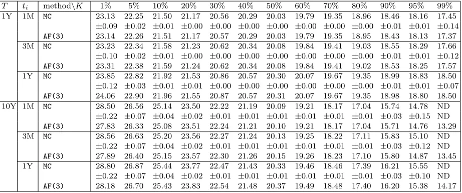
⊲benchmark. As a benchmark, we use Monte Carlo methods with a variance reduction technique (see chapter 4 in [8] for example). The simulated variable is (eXti+T−Xti−K)+ and we use the Black-Scholes control variate
(eXtiBS+T−X BS
ti −K)+−E[(eX BS ti+T−X
BS
ti −K)+] where XBS
t = x0+νWt− 12ν2t, the latter expectation being
computed with the Black-Scholes formula. Then we translate the results in terms of implied volatilities. We execute the simulations with 107sample paths and a time discretization of 300 steps per year using C++ on a
Intel(R) Core(TM) i5 [email protected] with 4 GB of ram. We report in Table 2 the estimations of the forward implied volatilities obtained with Monte Carlo (MC) indicating the half-width of the related 95%-symmetric
confidence interval and with the third order approximation formula (AF(3)). Sometimes for extreme strikes, we
report ND in the tabular because the corresponding price approximation does not belong to the non-arbitrage interval.
⊲Accuracy results. Globally the results are very good with a maximum error of around 50 bps1forT = 10Y and extreme strikes. But for such strikes, the MC estimate is questionable because of the large confidence
intervals. The errors become higher whenti+T or|k|increases and fork≈0 the results turn to be excellent with errors around 1 bp or less for T = 1Y and around 3 or 4 bps for T = 10Y. Excepting the two extreme strikes, errors are generally smaller than 15 bps what is very satisfying. The quite important errors in extreme strikes are probably due to the Vega close to zero in these areas. We should mention that in term of prices, the approximations are extremely accurate with errors close to 1 bp for the whole set of parameters.
Table 2. Hyperbolic model (β= 0.5, ν= 0.2): forward implied volatilities in % with MCand AF(3).
T ti method\K 1% 5% 10% 20% 30% 40% 50% 60% 70% 80% 90% 95% 99%
1Y 1M MC 23.13 22.25 21.50 21.17 20.56 20.29 20.03 19.79 19.35 18.96 18.46 18.16 17.45
±0.09 ±0.02 ±0.01 ±0.00 ±0.00 ±0.00 ±0.00 ±0.00 ±0.00 ±0.00 ±0.01 ±0.01 ±0.14
AF(3) 23.14 22.26 21.51 21.17 20.57 20.29 20.03 19.79 19.35 18.95 18.43 18.13 17.37
3M MC 23.23 22.34 21.58 21.23 20.62 20.34 20.08 19.84 19.41 19.03 18.55 18.29 17.66 ±0.10 ±0.02 ±0.01 ±0.00 ±0.00 ±0.00 ±0.00 ±0.00 ±0.00 ±0.00 ±0.01 ±0.01 ±0.12
AF(3) 23.31 22.38 21.59 21.24 20.62 20.34 20.08 19.84 19.41 19.02 18.53 18.25 17.57
1Y MC 23.85 22.82 21.92 21.53 20.86 20.57 20.30 20.07 19.67 19.35 18.99 18.83 18.50 ±0.12 ±0.03 ±0.01 ±0.01 ±0.00 ±0.00 ±0.00 ±0.00 ±0.00 ±0.00 ±0.01 ±0.01 ±0.07
AF(3) 24.06 22.90 21.96 21.55 20.87 20.57 20.31 20.07 19.67 19.35 18.98 18.80 18.50
10Y 1M MC 28.50 26.56 25.14 23.50 22.22 21.19 20.09 19.21 18.17 17.04 15.74 14.78 ND
±0.22 ±0.07 ±0.04 ±0.02 ±0.01 ±0.01 ±0.01 ±0.01 ±0.01 ±0.01 ±0.03 ±0.15 ND
AF(3) 27.83 26.33 25.08 23.51 22.24 21.21 20.10 19.21 18.17 17.04 15.71 14.76 13.29
3M MC 28.56 26.63 25.20 23.56 22.27 21.24 20.13 19.25 18.22 17.11 15.83 15.10 ND
±0.22 ±0.07 ±0.04 ±0.02 ±0.01 ±0.01 ±0.01 ±0.01 ±0.01 ±0.01 ±0.03 ±0.12 ND
AF(3) 27.89 26.40 25.15 23.57 22.30 21.26 20.15 19.26 18.23 17.10 15.80 14.87 13.45
1Y MC 28.80 26.87 25.44 23.77 22.47 21.43 20.33 19.46 18.46 17.39 16.21 15.55 ND ±0.22 ±0.07 ±0.04 ±0.02 ±0.01 ±0.01 ±0.01 ±0.01 ±0.01 ±0.01 ±0.03 ±0.10 ND
AF(3) 28.18 26.70 25.43 23.83 22.54 21.48 20.37 19.49 18.48 17.40 16.20 15.38 14.17
References
[1] E. Benhamou, E. Gobet and M. Miri. Smart expansion and fast calibration for jump diffusion.Finance and Stochastics, 13(4): 563-589, 2009.
[2] L. Bergomi. Smile dynamics II.Risk, 67-73, 2005. [3] L. Bergomi. Smile dynamics III.Risk, 90-96, 2008.
[4] P. Beyer and J. Kienitz. Pricing Forward Start Options in Models Based on (Time-Changed) Levy Processes.Preprint
available on SSRN, 2008.
[5] R. Bompis and E. Gobet, Asymptotic and non asymptotic approximations for option valuation, in Recent
Develop-ments in Computational Finance: Foundations, Algorithms and Applications, T. Gerstner and P. Kloeden, eds., World
Scientific Publishing Company, 2012.
[6] D. Brigo and F. Mercurio.Interest Rate Models Theory and Practice. Springer Finance, 2nd edition, 2006. [7] J. Gatheral.The Volatility Surface, a Practioner’s Guide. Wiley Finance, 2006.
[8] P. Glasserman.Monte Carlo Methods in Financial Engineering. Springer, 2003.
[9] P. S. Hagan, D. Kumar, A. S. Lesniewski, and D. E. Woodward. Managing smile risk.Willmott Magazine, 84-108, 2002. [10] G. Hong. Forward Smile and Derivative Pricing.Preprint2004.
[11] P. Jackel. Hyperbolic local volatility.Preprint, 2006.
[12] A. Jacquier and P. Roome. Asymptotics of forward implied volatility.Preprint available on arxiv, 2012.
[13] S. Kruse and U. Nogel. On the pricing of forward starting options in Hestons model on stochastic volatility.Finance
and Stochastics, 9(2): 233–250, 2005.
[14] V. Lucic. Forward-start options in stochastic volatility models.Wilmott Magazine, 2003.