Camparison of Numerically Stability of Two Algorithms for the Calculation of Variance

(1)

Camparison of Numerically Stability of Two Algorithms

for the Calculation of Variance

D. Rostamy

*

and E. Yaghesh

Department of Mathematics, Faculty of sciences, University of Imam Khomeini International University, Qazvin, Islamic Republic of Iran

Received: 19 January 2010 / Revised: 7 August 2010 / Accepted: 24 August 2010

Abstract

In descriptive statistics, there are two computational algorithms for determining

the variance

S

2

, of a set of observations

{ }

x

i ni=₁

:

Algorithm 1:

S

2

=

2 1

1

n

i i

x

n

-

å

=

-

2

1

n

x

n

-

,

Algorithm 2:

S

2

=

1

n

-2 1

( )

n

i i

x

=

-å

,

where

1 n

i i

x

=

å

. It is interesting to discuss, which of the above formulas is

numerically more trustworthy in machine numbers sets. I this paper, based on

total effect of rounding error, we prove that the second Algorithm is better than

the first Algorithm. Numerical experiments show the efficiency of Algorithm 2.

Keywords: Computational statistics; Round off error; Error analysis

*_{Corresponding author, Tel.: +98(021)44802601, Fax: +98(021)44802601, E-mail: [email protected]}

Introduction

The accuracy of results of calculations is a paramount goal in numerical analysis. For computing error analysis in a computational algorithm, sources of error are usually classified as follows:

1. Error in input data, 2. Round off errors, and 3. Approximation errors.

The stability analysis of a numerical method is related to the above sources of error if the amount of the total error is very small [10]. Different strategies for error analysis were investigated by von Neumann and Goldstein [8], Rademacher [9], Scarborough [12],

Ashenhurst and Metropolis [1], Wilkinson[16-18], Henrici [4], Moore [7], Kulisch [6], Knuth [5], Sterbenz [14], Bauer and Coworkers [2], [3], and Stauning [13].

Let us denote the set of machine numbers by F such that ( see [11], [14], [15]):

(

) { }

( )

1

, , , 0

: 1 ,s e m i i i

m L U

x x

b

b a b

-=

= =

ì _Î _{= -} ü

í ý

î

å

þ

È

F F R

where the set of floating point numbers with m significant digits, base b 2 , 0 ,³ a₁ ¹ 0£a £_i b -1,

1, , , 0,1

(2)

U , eÎZ , LÎ_Z and UÎ_Z. Therefore, it is clear that the members of F are finite and the cardinality of

(

b, , ,m L U

)

F is

(

)(

)

1

2 1 1 m 1.

Card_F₌ U L_{- +} b_- b - ₊

The elements of _F are called the machine numbers. If x Î F then we have to define the following mapping:

: , ,

rd D F R® DÌ

where rd(x)= x(1+ ε), | ε |≤ eps for all x ∈ D and eps = β

2 m

b

-é ù ´ ê ú

ë û is called the machine precision or the

machine epsilon.

On the other hand, we have observed that the results of arithmetic operations as ± ´ ¸ ¼ , , , cannot be expected to reproduce the arithmetic operations on ._F

We recall that if e < L or e > U then we have the definition of underflow and overflow, respectively.

Also, we consider an algorithm such as y =j

( )

x , that x and y are input and output of j, respectively. Therefore, its sequence of elementary operations gives rise to a decomposition of j into a sequence of elementary maps

( )r (r 1) ( )0

j ₌ j _oj - _{o o}_¼ j

( )

1

0 1

, ,

j

r

n i

i i j

n m

r

D D D

D D D

j

+

®

= Í

= Í =

R

R R

where characterize the algorithm. An algorithm for computing the function _j :_D _®_Rm _D , _Í_Rn,_{for a}

given ( , , )₁ T n

x = x ¼ x ÎD corresponds to a decomposition of the map j into elementary maps _ji _, and leads from _x(0)_{:= x via a chain of intermediate}

results

( )

0 (0) (0)

(1)( )r r (r 1) _,

x x x

x x x y

j

j +

= =

® ¼ ® = @

®

to a approximation of the result y. We assume that every i

j is continuously differentiable on Di. Now let us denote _yi _{the "remainder map" by:}

( ) ( 1) ( )

( )i r r i _: m_, _{0, ,} i

D i r

y ₌j j - _¼ j _® ₌ _¼

o o o R

then _y( )0 _º_j_{with floating-point arithmetic, input and}

round off errors will perturb the intermediate result

( )i

x . Considering these perturbations, we finally arrive at the following formula which describes the effect of the input errors Δx and the round off errors a_i on the result _{( )}_y _@_x(r+1) ₌_j _x _:

( )

( 1)

1 (1)

1 ( )

1

Δ Δ

Δ

. r

r r

y x

D x x D x

D x

j y a

y a a

+

=

+ + ¼

+ +

¡

(1)

The quantity a_i₊₁ can be interpreted as the absolute runoff error newly created when _ji_{is evaluated in} floating-point arithmetic, and the diagonal elements of

1

i

E + can be similarly interpreted as the corresponding

relative round off errors. The notation _¡ instead of = , which has used occasionally before, is meant to indicate that the corresponding equations are only a first order approximation, they do not take quantities of higher order Δ 's into account.

1 2 1

0 0 0

, ,

0 0 0

i j

n

E eps

e e

+

æ ö

ç ÷

= £

ç ÷

è ø

L M M M O M

L

( 1) 1 1 i .

i E xi

a +

+ = +

If one selects a different algorithm for calculating the same result j

( )

x , (in other words a different decomposition of j into elementary maps), then

Δ

Dj x remains unchanged; the Jacobian of the matrix i

Dy ,which measures the propagation of round off, will be different, however, and so the total effect of rounding error will be,

(1) ( )

1 1.

r

r r

Dy a + ¼+Dy a +a ₊ (2)

Definition 1. An algorithm is called numerically more

trustworthy than another algorithm for calculating

( )

x

j if, for a given data set x, the total effect of

rounding error (2) smaller for the first algorithm compared to that of the second one.

Outline of this paper is as follows. First we compute Δ

(3)

Computation of Dφ xΔ for Two Algorithms

Proposition 1. The terms Dj D. x are unchanged for two algorithms.

Proof. In Algorithm 1, we have the following statement:

2

1

Δ .Δ

2( ) 2( )

.

1 1

n

S D x

x x x x

x x

n n

j

= =

-

-D +¼+ D

-

-(3)

If we write,

2 2 2

1 2 2 1 1 2 2 1 1 1 1 1 1 ( ) 1 ( ) 1 1 n i i n n i i i i n n i i i i

S x n x

n

x n x

n n x x n n n j = = = = = æ ö

= = _ç - _÷

- è ø

æ ö

= _ç - _÷

- è ø

æ ö ç ÷ = -ç ÷ -è ø

å

and

(

)

1 1 1 2 1 1 2

1 ₂ ₂ _,2 ₂ _,

1

, 2 2

2 , , , , 1 n n i i i i n i i n n D x x x x

n n n

x x

n

x x x x x x

n j = = = = æ

ç _-

-ç -è ö ÷ ¼ -÷ ø

= - - ¼

-å

å

Then (1) is true. Also, for Algorithm 2 we can show (1) is true. We consider

2 2 1 2 1 1 2 1

1 ₍ ₎

1 1 1 n i i n n n

S x x

n x x x n n x x x n j = æ ö

= = _ç - _÷

- è ø

æ_æ _+¼+ _ö

= _çç_ç - _÷ +¼

- _èè ø

ö +¼+

æ ö

+_ç - _{÷ ÷}÷

è _{ø ø}

å

and 1 1 1 2 1 1 1 1 2 1 1 1 1 1 2 1 1 1 1 1 n n n n n n n n x x x n n x x x n n x x x n n D n x x x n n x x x n n x x x n n j

ææ _- +¼+ öæ _- ö ö

çç_è _÷è_øç ÷_ø ÷

ç ÷

ç _æ _+¼+ _öæ _ö ÷

+ - - +¼

ç _ç _{÷è ø}_ç _÷

è ø

ç

ç _æ _+¼+ _öæ _ö

ç +_ç - _÷_ç- _÷

ç è øè ø

ç

= _ç

-çæ _- +¼+ öæ_- ö

çç _{÷è ø}ç ÷

è ø

ç

ç _æ _+¼+ _öæ _ö

+ - - +¼

ç _ç _{÷è ø}_ç _÷

è ø

ç

ç _æ _+¼+ _öæ _ö

ç +_ç - _÷_ç - _÷

ç _è _ø_è _ø

è ø M T ÷ ÷ ÷ ÷ ÷ ÷ ÷ ÷ ÷ ÷ ÷ ÷ ÷ ÷ ÷÷

(

)

(

)

(

)

(

)

1 2 1 1 1 1 1

2 _,

1 1 1 1 T n i i n n i i

x x x x

n n

n

x x x x

n n

=

-=

ææ _- ö _- _{+ -}æ ö _- ö

çç ÷ ç ÷ ÷

è ø è ø

ç ÷

=

- ç ÷

æ ö æ ö

ç _- _- _{+ -} _- ÷

ç ÷ ç ÷

ç_è _ø _è _ø ÷

è ø

å

M

then we have:

(

)

(

)

(

)

(

)

2 1 1 2 1 1 Δ .Δ

2 _{[ 1} 1 1

1 1 1 1 ] n i i n

n i n

i

S D x

x x x x x

n n n

x x x x x

n n j = -= = =

ææ _- ö _- _{+ -}æ ö _- ö_{D + ¼}

çç ÷ ç ÷ ÷

- èè ø è ø ø

ææ ö æ ö ö

+_ç_ç - _÷ - + -_ç _÷ - _÷D

è ø è ø

è ø

å

(

) (

)(

)

(

)(

)

1 1 2 1 1 2

1 ( ) Δ

1

1 ( ) Δ

n

i i

n

n i n

i

n x x x x x

n n

n x x x x x

=

-=

éæ ö

= _êç - - - - _÷ +¼

- _ë_è _ø

ù

æ ö

+_ç - - - - _÷ _ú

è ø û

å

(

) (

)(

) (

)

(

)(

) (

)

(

)

1 1 1

2 ₁ _)Δ

1

1 n n Δ n

n x x x x x

n n

n x x x x x

= _éë - - - - +¼

-ù

+ - - - - _û

(

) (

1

)

1

(

)

2

Δ Δ ,

1 n x x x n xn x xn

n n

= é_ë - +¼+ - ù_û

-hence, proof is completed. □

Computation of the Total Effect of Rounding Error for Algorithms

(4)

elementary maps. In fact, in each stage only one computation will be done and we will follow algorithms step by step by elementary maps.

If we consider Algorithm 1, then we can state it by the following decomposition

(0 ) (1)

( )

1 1

(0) (1) (2)

2 1 1 1 ( ) 2 1 2 1 2 2 2 n n n n n n n x x

x x x

x x x x x x x x x x x x j j j æ ö

æ ö ç ÷

ç ÷ _ç _÷

=_ç _÷® =_ç _÷®

ç ÷ _ç _÷

è ø

æ ö

æ ö ç ÷

ç ÷ _ç _÷

ç ÷

= ¼ =ç ÷®

ç ÷ _ç _÷

è ø ç_è ÷_ø

M M

M

( 2 1)

( 2 )

1 2 3

1

( 1) (2 1) 2 (2 ) 1 2 1 2 2 2 2 1 2 n n n i i

n n n

n

x x

x x

x x x x

x x x x x x x j j -+ = + -æ ö æ ö ç ÷ ç ÷ ç ÷ ç ÷ ç ÷ ç ÷

=ç ÷¼ = ®

ç ÷

ç ÷ _è _ø

ç ÷

è ø

æ ö

ç ÷

=_ç _÷ ®

ç ÷ ç ÷ è ø

å

M M M ( ) ( ) ( ) ( ) ( )

2 1 2 2

2 2

2 1 1 2 2 1

2 2

2 2 2 2 3 1 2

2 n n n n n n n n x nx x x x x x x nx x x x x

j + j +

+ +

+

æ ö æ ö

ç ÷ ç ÷

=_ç _÷ ® =_ç _÷ ®

ç ÷ ç ÷

è ø è ø

æ ö

ç ÷

+

ç ÷

= ç ÷

ç ÷

è ø

M M

M

(3 1) ( 3 2)

2

(3 1) (3 2) 2 2 2

1 1

(3 3) 2 2 1

1

. 1

n _n n

n n n i i i i n n i i nx

x x x nx

x

x x nx

n

j + j +

+ + = = + = æ ö ç ÷ = ® = - ® ç ÷ è ø =

-å

å

Also, the following decomposition is given for Algorithm 2. ( ) ( ) ( ) ( ) ( ) ( ) 0 1 1 1 0 1 1 2 1 1 1 1 n n n n n n n n i i x x x x x x x x x x

x x x

x x x j j -= æ ö

æ ö _ç _÷

ç ÷ _ç _÷

=_ç _÷® =_ç _÷¼

ç ÷ _ç _÷

è ø ₊

è ø æ ö æ ö ç ÷ ç ÷ ç ÷ ç ÷ ç ÷

= ® =_ç _÷

ç ÷

è ø

ç ÷

è

å

ø

M M M _M ( ) ( ) ( ) ( ) ( )

(

)

2 1 2 1 2 1 1

2 2 1 2

n n n n n n n n x x x x x x x x x x x x x x x x x x j j + + -æ ö ç ÷ ç ÷ ç ÷

® = ¼

ç ÷

è ø

æ _- ö

-æ ö ç ÷

-ç ÷ ç ÷

=_ç _÷® =_ç _÷

ç _- ÷ _ç _÷

è ø _ç _- _÷

è ø M M M ( )

(

)

(

)

( ) ( )

(

) (

)

(

)

(

)

3 2 1 3 2 2 2 1 2 2

3 1 3

2 n n n n n x x x x x

x x x x

x x

x

x x

j

+

æ _- ö

ç ÷

=ç ÷®

ç ÷

ç _- ÷

è ø

æ _- ₊ _- ö

ç ÷

ç - ÷

=_ç _÷¼

ç ÷

ç _- ÷

è ø M M ( ) ( ) ( ) 4 1

4 1 2

1 4 2 1 ( ) 1 ( ) . 1 n n n i i n n i i

x x x

n j -= = = - ® =

-å

å

It is concluded that if we have n observations

{ }

1

n i i

x ₌ then using Algorithm1 leads to (3n+3) elementary maps and using Algorithm 2 leads to (4n) elementary maps.

Total Effect of Rounding for Algorithm 1

Proposition 2. A bound for the total effect of rounding

error for Algorithm 1 is as follows:

2 2

2 1

2 2 .

1 n

x x

A nx y eps

n

é æ +¼+ ö ù

£ê ç _- ÷+ + ú

ê è ø ú

(5)

Here, we assume A:= Total effect of rounding error for Algorithm 1, such that

2 2

2 1

1 1

2

2 3

1

2

1 1

1 _.

1

n

n n

n

i n n

i

x x

A nx

n n

x y

n

e e e

e e

+

+ +

=

= +¼+

--

-æ ö

+ _ç _÷ +

- è

å

ø

Proof. If we consider Algorithm 1 then for simplicity we can write:

( )0

(

)

1, , n ,

x =x = x ¼ x

( )0

( )

( )0 ( )1

(

2 2

)

1 , , n ,

x x x x

j = = ¼

( )1

( )

( )1 ( )2 2 1

, ,

n

i i

x x x x

j

=

æ ö

= _{= ç} _÷

è

å

ø

( )2

( )

( )2 ( )3 2 2 1

1

, . 1

n

i i

x x x n x

n

j

=

æ ö

= = _ç _÷

- è

å

ø

Therefore, we have: ( )2 ( )1 ( )0_,

j j= oj oj

( )

1

(3) (1)

1 2

(2)

2 3

Δy Δx D x Δx D x

D x

j y a

y a a

= +

+ +

¡

and

( )

( 0) (1)

2

2 1 1

(0) (1) 2

2

(2) ₁ (3 3) 2 2 2

1

1 _.

1 n n

n _n

n i

i

i i

x x

x

x x x nx

n x

j j

j + =

=

æ ö

æ ö ç ÷

ç ÷ ç ÷

=_ç _÷® =_ç _÷®

ç ÷ _ç _÷

è ø _ç _÷

è ø

æ ö

ç ÷

= ® =

-ç ÷

-è ø

å

M M

hence,

( )

(

)

2 1 0

1, , n ₂ , n

x

x x

j

æ ö

ç ÷

¼ _{= ç} _÷

ç ÷

è ø

M

( )1

(

)

₁ 1

1

, , ,

n i i n

n

u

u u

u

j =

+

æ ö

ç ÷

¼ =

ç ÷

è ø

å

( )2

( )

_, 1

(

2

)

_,

1

u v u nv

n

j =

-( )

(

)

( ) ( )

(

)

( )

1 2 1

1 1

2

1 1

2 1 1

, , , ,

,

1 _,

1

n n

n

i n i

n

i n

i

u u u u

u u

u nu

n

y j j

j

+ +

+ =

¼ = ¼

æ ö

= _ç _÷

è ø

æ ö

= _ç - _÷

- è ø

å

o

( )1

(

)

(

)

1 1

1

, , 1, ,1, 2 ,

1

n n

D u u nu

n

y ¼ ₊ = ¼ - ₊

-( )

( )

( ) ( )

(

)

(

)

1 1 1 2 2

1 , , ,

1 _{1, ,1, 2} _,

1

n

D x D x x x

nx n

y = y ¼

= ¼

-( )2

( )

_, ( )2

( )

_, 1

(

2

)

_,

1

u v u v u nv

n

y =j =

-( )2

( )

_, 1

(

_{1 2}

)

_,

1

D u v nv

n

y =

-( )2

( )

( )2 ( )2 2

(

)

1

, 1 2 .

1

n

i i

D x D x x nx

n

y y

=

æ ö

= _ç _÷=

-è

å

ø

Moreover, we have:

( )0

( )

( )0 ( )0

( )

( )0

(

2 2

)

1 1 1, , , 1 ,

T

n n n

x x x x x

j -j = =a e ¼ e e ₊

( )1

( )

( )1 ( )1

( )

( )1 2

2 2

1

,0 , T n

i n i

x x x

j j a e ₊

=

ææ ö ö

- = = çç ÷ ÷

è ø

è

å

ø

( )2

( )

( )2 ( )2

( )

( )2

3 3 2 2

3 1

1

. 1

n

i n

i

x x y

x nx

n

j j a e

e

+

+ =

- = =

æ ö

= _ç - _÷

- è

å

ø

So, we can write

( )

( )1

( )

( )1 ( )2

( )

( )2

1 2 3

Δ

Dj x x +Dy x a +Dy x a +a =

( )

2 2

1 1

2

2 3 1

1

Δ ( 2 )

1

1 _.

1

n

i i n

i n

i n n

i

D x x x nx

n

x y

n

j e e

e e

+ =

+ +

=

+

-æ ö

+ _ç _÷ +

- è ø

å

Therefore, the proof is completed. □

Total Effect of Rounding Error for Algorithm 2

Proposition 3. A bound for the total effect of rounding

error for Algorithm 2 is as follows:

2 2

1

( ) ( )

.

1 1

n

x x x x

B y eps

n n

é - - ù

£_ê +¼+ + _ú

-

(6)

Here, we assume B:= Total effect of rounding error for Algorithm 2, such that

2 2

1

2 1 3

( ) ( )

.

1 1

n

n n

x x x x

B y

n e n e + e +

-

-= +¼+ +

-

-Proof. If we consider Algorithm 2 then for simplify we can write:

( )0

(

)

1, , n ,

x =x = x ¼ x

( )0

( )

( )0 ( )1

(

)

1, , n, ,

x x x x x

j = = ¼

( )1

( )

( )1 ( )2

(

2 2

)

1

( ) , ,( n ) ,

x x x x x x

j = = - ¼

-( )2

( )

( )2 ( )3 2 1 1 ( ) . 1 n i i

x x x x

n

j

=

= =

--

å

Therefore, we have: ( )2 ( )1 ( )0_,

j j= oj oj

( )

( ) ( )

( )

1 (3) (1) 1 2 (2) 2 3

Δy Δx D x Δx D x

D x

j y a

y a a

= +

+ +

¡

and we can conclude

( ) ( ) ( ) ( ) ( )

(

)

(

)

( ) ( ) 0 1 2 1 1 0 1 2 1

2 3 2

1 2 1 ( ) . 1 n n n i i n x x x x x x x x x

x x x x

n x x j j j = æ ö

æ ö _ç _÷

ç ÷ _ç _÷

=_ç _÷® =_ç _÷®

ç ÷ _ç _÷

è ø

æ _- ö

ç ÷

=ç ÷® =

-ç ÷

ç _- ÷

è ø

å

M M

M

Hence, we have

( )

(

)

1 0

1, , n ,

n x x x x x j æ ö ç ÷ ç ÷ ¼ = ç ÷ ç ÷ è ø M ( )

(

)

(

)

(

)

2 1 1 1 1 2 1 , , , n n n n u u u u u u j + + +

æ _- ö

ç ÷

¼ = ç ÷

ç ÷

ç _- ÷

è ø

M

( )2

(

)

1 1 1 , , , 1 n n i i

v v v

n j = ¼ = -

å

( )

(

)

( ) ( )

(

)

( )

(

)

(

)

1 2 1

1 1 1

2 2

2

1 1 1

, , , ,

, ,

n n

n n n

u u u u

y j j

j

+ +

¼ = ¼

= - ¼

-o

(

)

(

)

(

)

(

)

2 1 1 2 2

1 1 1

1 1 1 , 1 n i n i

n n n

u u

n

u u u u

n + = + + æ ö -ç ÷

- è ø

= - +¼+

-å

( )

(

)

(

)

(

)

(

)

(

)

1

1 1 1 1

1

, , 2 , ,

1

2 , 2 , , 2

n n

n n n n n

D u u u u

n

u u u u u u

y ₊ ₊

+ + +

¼ = - ¼

-- - - ¼ -

-(

)

(

1 1 1 1 1

)

2

, , , ,

1 u un un un nun u un

n + + +

= - ¼ - - +¼+

-( )

( )

( ) ( )

(

)

(

)

(

)

(

)

1 1 1 1 1 1 1 , , , 2 , , , 1 2

, , ,0 , 1

n

n n

n

D x D x x x

x x x x nx x x

n

x x x x

n

y = y ¼

= - ¼ - - +¼+

-= - ¼

-( )2

(

)

( )2

(

)

1 1 1 1 , , , , , 1 n

n n i

i

v v v v v

n

y j

=

¼ = ¼ =

-

å

( )2

(

)

1

1 1

, , ( , , ),

1 1

n

D v v

n n

y ¼ = ¼

-

-( )2

( )

( )2 ( )2

(

2 2

)

1 ( ) , , ( ) 1 1 ( , , ). 1 1 n

D x D x x x x

n n

y = y - ¼

-= ¼

-

-Moreover, we have:

( )0

( )

( )0 ( )0

( )

( )0

(

)

1 0, ,0, 1 ,

T

x x x

j -j =a = ¼ e

( )

( ) ( )

( )

(

)

1 1 1 1 2

2 2

1 2 1

( ) , ,( n ) n T,

x x

x x x x

j j a

e e +

- =

= - ¼

-( )2

( )

( )2 ( )2

( )

( )2

3 2 2 2 1 1 ( ) . 1 n n i n i

x x y

x x

n

j j a e

e + + = - = = æ ö

= _ç - _÷

- è

å

ø

So, we can write

( )

( ) ( )

( )

1 (1) 1 2 (2) 2 3 Δ Δ ,

y D x x D x

D x

j y a

y a a

+

+ +

¡

( )

2

1 2

1

Δ Δ ( ) .

1

n

i i n

i

y D x x x x y

n

j e₊ e ₊

=

æ ö

+ _ç - _÷+

- è

å

ø

¡

(7)

Corollary 1. Comparing (4) and (5) we have:

2 2

1

( ) ( )

1 1

n

x x x x

y

n n

é - _+¼+ - ₊ ù

ê _- _- ú

ë û

£ ₂ 12 2 ₂ 2

1 n

x x

nx y

n

é æ +¼+ ö₊ ₊ ù

ê ç _- ÷ ú

ê è ø ú

ë û

This means that total effect of rounding for Algorithm 2 is less than total effect of rounding for Algorithm 1. Therefore, we can conclude that Algorithm 2 is numerically more trustworthy than Algorithm 1.

Results and Discussion

In what follows we run two algorithms on three sets of data. Also, we assume that the set of numbers is

(

10, 4, ,L U

)

=

F F . Our aim is to calculate the relative errors of the two algorithms in the set F=

(

10,6, ,L U

)

F .

Remark 1. e1 and e2 denote the relative error for

Algorithm 1 and 2, respectively.

Example 1. We assume that the set of observations is

x1=0.1256, x2=0.2347, x3=0.3511. In the set

(

10, 4, ,L U

)

=

F F we obtain x =0.2371 and in the set

(

10,6, ,L U

)

=

F F we obtain x =0.237133. The

variance and relative errors are shown n Table 1. Example 2. We assume that the set of observations is

x1=0.1123, x2=0.1234, x3=0.1356. In the set

(

10, 4, ,L U

)

=

(

10,6, ,L U

)

=

F F we obtain x =0.123767. Therefore,

we have Table 2:

Example 3. We assume that the set of observations is

x1=0.1113, x2=0.1124, x3=0.1135. In the set

(

10, 4, ,L U

)

=

(

10,6, ,L U

)

=

F F we obtain x =0.112400. Therefore,

we have Table 3:

We have proven that the total effect of rounding error of Algorithm 2 is less that the total effect of rounding error of Algorithm 1. Hence, we can conclude that Algorithm 2 is numerically more trustworthy. We should notice that for large n, computing 2

1

n

i i

x =

å

and

2 1

( )

n

i i

x x

=

-å

is a numerical problem and we should add small data first to prevent large errors.

Table 1. Comparison between two Algorithms for example 1 Alg. 1 Alg. 2 Variance of observations

in F(10,4,L,U)

2 1

S =0.0128 2

2

S =0.0127

Variance of observations in F(10,6,L,U)

2 1

S =0.012717 2

2

S =0.012717

Relative error

in F(10,6,L,U) e1=0.006527 e2=0.001337

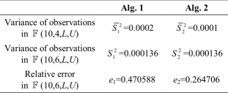
Table 2. Comparison between two Algorithms for example 2

Alg. 1 Alg. 2 Variance of observations

in F(10,4,L,U) S12=0.0002 S22=0.0001

2 1

S =0.000136 2

2

S =0.000136

Relative error

in F(10,6,L,U) e1=0.470588 e2=0.264706

Table 3. Comparison between two Algorithms for example 3 Alg. 1 Alg. 2 Variance of observations

in F(10,4,L,U) S12=0.0001 S22=0.0000

2 1

S =0.000001 2

2

S =0.000001

Relative error

in F(10,6,L,U) e1=0.990000×10

2_{e2=0.100000×10}1

Acknowledgement

The authors wish to thank the referees and the editor for their useful comments and suggestions.

References

1.R. L. Ashenhurst & N. Metropolis, Un-normalized

floating-point arithmetic, J. Assoc. Comput. Math. 6:415-428 (1959).

2.F. L. Bauer, Computational graphs and rounding error,

SIAM J. Numer. Anal. 11: 87-96 (1974).

3.F. L. Bauer, J. Heinhold, k. Samelson & R. Sauer, Modern Rechenanlagen, Teubner, Stttgart, (1965).

(8)

Wiley, New York, (1963).

5.D. E. Knuth, The Art of Computer programming,

Semi-numerical Algorithms, Vol. 2, Addison-Wesley, Reading, MA,(1969).

6.U. Kulisch, Grundzgue der Intervallrechning,in: D.

Lauugwitz (Ed.), Uberblicke Mathematik, Vol. 2, Bibliographihes Institut Mannheim, pp.51-98 (1969). 7.R. E. Moore, Interval Analysis, Prentice-Hal, Englewood

Cliff, NJ, (1966).

8.J. Von Neumann & H. H. Goldstein, Numerical inverting of matrices, Bull. Amer. Math,Soc. 53: 1021-1099 (1947).

9.H. A. Rademacher, On the accumulation of errors in

processes of integration on the high-speed calculating machines, in: Proceedings of a Symposium on Large Scale Digital Calculating Machinery, Annals Comput. Labor. Harvard University, Vol. 16: pp. 176-185 (1948).

10.M. Rosenbaum, Integrated volatility and round-off error. Bernoulli 15: No 3, 687-720 :(2009).

11.D. Rostamy V. F., A Stochastic Partial Differential Equation for Computational Algorithms, 159: 429-434 (2004).

12.J. b. Scarborough, Numerical Mathematical Analysis,

second ed. , Johns Hopkins Press, Baltimore, MA,(2002). 13.O. Stauning, Automatic Validation of Numerical Solutions,

Ph. D. Thesis, Technical University of Denmark, Lyngby, (1997).

14.F. H. Sterbenz, Floating Point Computation, Prentice-Hall, Englewood Cliffs, NJ, (1974).

15.J. Stoer & R. Bulirsch, Introduction to Numerical Analysis, Springer-Verlag, New York,(2002).

16.J. H. Wilkinson, Error analysis of floating-point

Computation, Numer. Math. 2(1960)219-340.

17.J. H. Wilkinson, Rounding Errors in Algebraic Processes, Wiley, New York, (1963).

18.J. H. Wilkinson, The Algebraic Eigen-value Problem,