ESAIM: PROCEEDINGS,December 2012, Vol. 38, p. 429-455 F. Coquel, M. Gutnic, P. Helluy, F. Lagouti`ere, C. Rohde, N. Seguin, Editors
F
EEL++: A COMPUTATIONAL FRAMEWORK FOR GALERKIN METHODS AND
ADVANCED NUMERICAL METHODS
C
HRISTOPHEP
RUD’
HOMME2, V
INCENTC
HABANNES1, V
INCENTD
OYEUX3, M
OURADI
SMAIL3, A
BDOULAYES
AMAKE1 ANDG
ONCALOP
ENA4Abstract. This paper presents an overview of a unified framework for finite element and spectral element methods in 1D, 2D and 3D inC++called FEEL++. The article is divided in two parts. The first part pro-vides a digression through the design of the library as well as the main abstractions handled by it, namely, meshes, function spaces, operators, linear and bilinear forms and an embedded variational language. In every case, the closeness between the language developed in FEEL++ and the equivalent mathematical ob-jects is highlighted. In the second part, examples using the mortar, Schwartz (non)overlapping, three fields and two fictitious domain-like methods (the Fat Boundary Method and the Penalty Method) are presented and numerically solved in the scope of the library.
1. I
NTRODUCTIONLibraries to solve problems arising from partial differential equations (PDEs) through generalized Galerkin methods are a common tool among mathematicians and engineers. However, most libraries end up specializing in a type of equation, e.g. Navier-Stokes or linear elasticity models, or a specific type of numerical method, e.g. finite elements. The increasing complexity of differential models and the implementation of state of the art robust numerical methods, demand from scientific computing platforms general and clear enough languages to express such problems and provide a wealth of solution algorithms available in a minimal amount of code but maximum mathematical control. There are many freely available libraries which offer the capabilities described previously to a certain extent. To name a few: the Freefem software family [24,44], the Fenics project [36,37], Getdp [19], DUNE [15] or Getfem++ [49], or libraries or frameworks such as deal.II (C++) [6], Sundance (C++) [38], Analysa (Scheme) [2]. Either they rely on a domain specific language (Python, the freefem language, ...) when it comes to describe the PDE to solve, or they are geometry or dimension dependent, or they are not so expressive with respect to the mathematics, i.e. the mathematics are hidden by programming details.
The library we present in this paper, called FEEL++,Finite Element Embedded Language inC++, see [45,46] for the initial papers, provides also a clear and easy to use interface to solve complex PDE systems. It aims at bringing the scientific community a tool for the implementation of advanced numerical methods and high performance computing. Some recent applications of FEEL++ to multiphysics problems can be found in the literature, see [13,17,41–43].
Two main aspects in the design of the library are to (i) have the syntax, semantics and pragmatics of the library very close to the mathematics, and (ii) have a small manageable library that makes use wherever possible of established libraries (for linear system solves, for instance). While the first aims at creating a high level language powerful enough to describe solution strategies in a simple way, the second helps with the maintenance of the code delegating some procedures to frequently maintained third party libraries.
FEEL++ relies on a so-called domain specific embedded language(DSEL) designed to closely match the Galerkin mathematical framework. In computer science, DS(E)Ls are used to partition complexity and in our
1Laboratoire Jean Kuntzmann, Universit´e Joseph Fourier Grenoble 1, BP53 38041 Grenoble Cedex 9, France, Tel.: +33476635497, Fax:
+33476631263, e-mail:[email protected] [email protected] [email protected]
2Universit´e de Strasbourg / CNRS, IRMA / UMR 7501. Strasbourg, F-67000, France
3Universit´e Grenoble 1 / CNRS, Laboratoire Interdisciplinaire de Physique / UMR 5588. Grenoble, F-38041, France
e-mail:[email protected] [email protected]
4CMUC, University of Coimbra, Largo D. Dinis, Apartado 3008, 3001-454 Coimbra, Portugal, e-mail:
c
EDP Sciences, SMAI 2012
case the DSEL splits low level mathematics and computer science on one side leaving the FEEL++ developer to enhance them and high level mathematics as well as physical applications to the other side which are left to the FEEL++ user. This enables using FEEL++ for teaching purposes, solving complex problems with multiple physics and scales or rapid prototyping of new methods, schemes or algorithms. The goal is always to hide (ideally all) technical details behind software layers, provide only the relevant components required by the user or program-mer and enforce the mathematical language computationally between the users be they physicists, mathematicians, computer scientists, engineers or students. The DSEL approach has advantages over generating a specificexternal
language: (i) interpreter/compiler construction complexities can be ignored, (ii) libraries can concurrently be used which is often not the case of specific languages which would have to also develop their own libraries and library system, (iii) DSELs inherit the capabilities of the host language (e.g.C++).
The DSEL on FEEL++ provides access to powerful, yet with a simple and seamless interface, tools such as interpolation or the clear translation of a wide range of variational formulations into the variational embedded language. Combined with this robust engine, lie also state of the art arbitrary order finite elements — including handling high order geometrical approximations, — high order quadrature formulas and robust nodal configuration sets. The tools at the user’s disposal grant the flexibility to implement numerical methods that cover a large combination of choices from meshes, function spaces or quadrature points using the same integrated language and control at each stage of the solution process the numerical approximations.
Finally FEEL++ uses advancedC++ (e.g. template meta-programming) and in particular the latest standard C++11 that provides very useful additions such as type inference —autoanddecltypekeywords which are used throughout the paper. — FEEL++ also uses the essential BoostC++libraries [1]: in this paper most scripts displayed use explicitly the Boost Parameter library1enabling a very powerful programming interface namely
named parameters(required and optional) given in a random order to a class — template parameters —, a class member function or a free function. This library enhances tremendously readability, expressivity and ease of use of the code. Many other Boost libraries are used in FEEL++, some are listed in this document.
The paper is organized in two parts. The first part describes an overview of the main abstractions and interfaces handled by the library. In section2we describe the basic ideas behind the construction of the reference element, finite elements defined therein and the geometrical transformation. Section 3shows how to handle and define meshes, function spaces, forms, functionals and operators. The variational embedded language is presented in section 4, with particular emphasis in the projection and integration procedures. The second part introduces several examples using the mortar, Schwartz (non)overlapping, three fields, see section5, and fictitious domain-like methods, see section 6, to illustrate the flexibility of the language. These methods are being developed within FEEL++ to be used, possibly concurrently, to solve multiphysics and/or multiscale problems within high performance computing environments.
2. P
OLYNOMIALL
IBRARYThe polynomial library is composed of various bricks: (i)the geometrical entities or convexes(ii)the prime basis in which we express subsequently the polynomials, (iii) the definition and construction of point sets in convexes (such as quadrature point sets) and finally(iv)polynomials and finite elements.
2.1.
Convexes
The supported convexes are simplices and hypercubes of topological dimensionn,n=1,2,3 lying inRdsuch thatn6d63. The convexes are described geometrically in a standard way in terms of their subentities (vertices, edges, faces, volumes), see for example [32], and provide the ability to iterate over the entities of a convex or of the same topological dimension inside a convex, e.g. iterate over the edges of a tetrahedron.
2.2.
Prime basis:
L
2Orthonormal Polynomials
In order to express polynomials in the convexes defined previously, we need to choose aprime basis, i.e., a basis in which all polynomial families are expressed. Often, the choice falls on the canonical basis (also known as themoment ormonomial basis). However, recent work by R.C. Kirby [33–35] proposed to use the Dubiner polynomials as a prime basis on the simplex. We extended these ideas on the hypercubes using the Legendre polynomials. Other interesting examples of prime basis being used are the Bernstein polynomials. Our framework uses the Dubiner or Legendre basis as the default prime basis. This choice simplifies the construction of finite elements due to the hierarchical andL2orthogonality properties these basis functions share. The choice of basis polynomials that are hierarchical allows for an easy extraction of a basis spanning a subspace of the polynomial
1http://www.boost.org/doc/libs/1_48_0/libs/parameter/doc/html/index.html
space (which corresponds to extract a range of coefficients), whereasL2orthogonality simplifies some operations like numerical integration or theL2 projection (which is explicit in this case). The use of these basis functions proved to provide much better numerical stability, see [41].
Details on the construction of the Dubiner polynomials can be found in [32] page 101. In practice, the prime basis is normalized.
2.3.
Point Sets on Convexes
Now we turn to the construction of point setsP defined on a convex K. Point sets are represented alge-braically by a matrix (rows are indexed by the coordinates while columns are indexed by the points) and they are parametrized by the associated convex and the numerical type. We recall that the convex is decomposed in vertices, edges, faces, volumes. A similar decomposition is done for the point sets: points are constructed and associated to their respective entities on which they reside. This is crucial when considering continuous and discontinuous Galerkin formulations.
The type of point sets supported are(i)the Equidistributed point set,(ii)the Warpblend point sets on simplices see [51],(iii)Fekete points in simplices, see [32],(iv)standard quadrature rules in simplices and finally(v)Gauss, Gauss-Radau and Gauss-Lobatto and combinations in simplices and hypercubes. It should be noted that the last family is constructed from the computation of the zeros of the Legendre polynomials on[−1,1]including eventually the boundary vertices−1, 1 for the Radau and Lobatto flavors.
Warpblend and Fekete points are used with nodal basis on simplices which, when constructed at these points, present much better interpolation properties (lower Lebesgue constant, see [32]). Note that the Gauss-Lobatto points are the Fekete points in hypercubes.
2.4.
Polynomial Set
After introducing in the previous sections the necessary bricks to the construction of polynomials on simplices and hypercubes, we now focus on the polynomial abstraction.
A polynomial setPis a template class parametrized by the prime basis in which it is expressed and the field type in which it has its values: scalar, vectorial or matricial. Its interface provides a number of operations such as evaluation and derivation at a set of points, extraction of polynomials or components (when theFieldTypeis
VectorialorMatricial) of a polynomial from a polynomial set .
One critical operation is the construction of the gradient of a polynomial (or a polynomial set) expressed in the prime basis. This usually requires solving a linear system where the matrix entries are given by the evaluation of the prime basis and its derivatives at a set of points. Again the choice of set of points is crucial here to avoid ill-conditioning and loss of accuracy. We choose Gauss-Lobatto points for hypercubes and Warpblend or Fekete points for simplices as they provide a much better conditioning for the underlying system matrix (a generalized Vandermonde matrix, see [41]).
2.5.
Finite Elements and Other Polynomial Basis
FEEL++ supports modal basis, e.g. Legendre or Dubiner, see [12,32], as well as finite elements (FE) following the standard definition, set in [14], as a triplet(K,P,Σ)whereKis a convex,Pthe polynomial space andΣthe dual space. We describe now some features of the finite element framework. The description ofKandPhas been presented previously and it remains to describeΣ.Σis a set of functionals (which can be identified as degrees of freedom) defined inPwith values inR,RdorRd×d. Several types of functionals can then be instantiated which merely require basic operations like evaluation at a set of points, derivation at a set of points, exact integration or numerical integration. Some examples of functionals satisfying such requirements are (1) evaluation at a point
x∈K,`x:p→p(x), (2) derivation at a pointx∈Kin the directioni,`x,i: p→∂∂xip(x), (3) moment integration associated with a polynomialq∈P(K),`q:p→R
Kpq.
A functional is represented algebraically by a vector whose entries result from the application of the functional to the prime basis in which we express the polynomials thanks to the bijection betweenL(P,R)andRdim(P). Then applying the functional to a polynomial is just a scalar product between the coefficient of this polynomial in the prime basis by the vector representing the functional. For example theLagrange elementis the finite element (K,P,Σ={`xi,xi∈X⊂K})such that`xi(pj) =δi jwherepjis a Lagrange polynomial andX={xi}is a set of points defined in the convexK, for example the Equidistributed, Warpblend or Fekete point sets. Other FE such asP1,2-bubble,RTkorNkpolynomials are constructed likewise though they require a more involved description.
2.6.
Geometry
To conclude this section, one important object that is constructed with the help of the polynomial library is the
geometric transformation. Indeed all polynomial set constructions are done on a reference convex, denoted ˆK, and the geometrical transformation maps it to a convex in the physical space which we denoteK. This map, denoted φKgeo, is theC1−diffeomorphism defined on ˆK⊂Rp,p=1,2,3 such that the image isK⊂Rd, i.e.φKgeo: ˆK−→K
forp6d63. This map is constructed and associated to each convexKin a computational meshTh, see section3. Notice that this last condition overpanddcovers a large spectrum of geometrical profiles. For instance, we handle lines or surfaces inR3. We refer the reader to section5.4for an example where this flexibility is exploited.
ˆ
x
ˆ
y
•
ˆ
x1
•
ˆ
x2
•
ˆ
x3
•
ˆ
x4
•xˆ5 •
ˆ
x6
ˆ
K
x y
• x1
• x2
• x3
• x4
•x5 •
x6
K
φKgeo(ˆx)
(φKgeo)−1(x)
The geometric transformation is constructed as a suitable linear combination of Lagrange polynomials and therefore it can be a polynomial of arbitrary degree, allowing thus meshes with elements that have curved edges/-faces, see [42,43]. Another consequence ofφKgeo being a polynomial of a degree the user can choose, is the possibility to define isoparametric (or subparametric or surparametric) finite elements, see [41,43]. Lets denote
kgeothe polynomial order of the Lagrange basis in whichφKgeois expanded. If there is no ambiguity, we keep the notationφKgeo, otherwise we use the notationφKgeo,k
geo.
The class that implements the definition and evaluation of the geometrical transformation also provides a func-tion to evaluate its gradient, automatic consequence ofφKgeo being an element belonging to a polynomial set. Another important transformation associated withφKgeois its inverse,(φKgeo)−1. In the case of an affine transforma-tion, the inverse is calculated explicitly. However, ifφKgeois nonlinear, the evaluation/differentiation of(φKgeo)−1 at a set of points is performed with the help of a nonlinear solver (we have used the nonlinear solver available in
PETScfor these calculations, see section3.2). The inverse transformation plays an essential role in providing an
interpolation tool, all the advanced numerical methods presented in sections5and6use this tool and hence the inverse geometrical transformation.
3. M
ESHES, F
UNCTIONS
PACES ANDO
PERATORSIn the previous section, we have described roughly the monodomain construction of polynomials. Now we turn to the ingredients for the multidomain construction and we start with the mesh mathematical description and associated data structures.
3.1.
Mesh Data Structures
LetΩ⊂Rd,d≥1, denote a bounded connected domain. We first need to introduce a suitable discretization of Ω,Ωh⊂Ω. Note that ifΩis a polyhedral domain thenΩh=Ω. We denote byTha finite collection of nonempty, disjoint open simplices or hypercubesTh={K=φKgeo(Kˆ)}forming a partition ofΩhsuch thath=maxK∈ThhK, withhK denoting the diameter of the elementK∈Th. We say that a hyperplanar closed subsetF ofΩis a mesh face if it has positive(d−1)-dimensional measure and if either there existK1,K2∈Thsuch thatF=∂K1∩∂K2 (andF is called aninternal face) or there existsK∈Thsuch thatF =∂K∩∂Ωh(andF is called aboundary face). Internal faces are collected in the setFhi, boundary faces inFhband we letFh:=Fhi∪Fhb. For allF∈Fh, we defineTF:={K∈Th|F⊂∂K}.For every interfaceF∈Fhi we introduce two associated normals to the elements inTF and we have nK1,F=−nK2,F, where nKi,F,i∈ {1,2}, denotes the unit normal toFpointing out of Ki∈TF. On a boundary faceF∈Fhb, nF=nK,Fdenotes the unit normal pointing out ofΩh. We also introduce (i) the set of boundary elementsThb={K∈Th |∂K∩∂Ω6=/0}, (ii) the set of internal elementsThi=Th\Thb, (iii) the setNhwhich collects the nodes of the mesh, (iv) whend=3,Ehwhich collects the edges of the mesh.
The collectionsTh,Fh,Eh,Nh, as well as the internal and boundary collections, are provided by our mesh data structure and stored using the the Boost.Multi index library2. The mesh entities (elements, faces, edges, nodes) are indexed either by their ids, the process id (i.e. the id given by MPI in a parallel context, by default the current process id) to which they belong, their markers (material properties, boundary ids. . . ) or their location (whether the entity is internal or lies on the boundary of the domain). Other indices could certainly be defined, however those previous four already allow a wide range of applications. Thanks to Boost.Multi index, it is trivial to retrieve pairs of iterators over the entity’s containers depending on the usage context. The pairs of iterators are then turned into a range, see Boost.Range3, to be manipulated by the integration, see section4.1, and projection,
see section4.2, tools. Table1summarizes some of the available ranges in the library.
Range iterators Description
elements(<mesh>) range iterator overTh
faces(<mesh>) range iterator overFh
edges(<mesh>) range iterator overEh
points(<mesh>) range iterator overNh
markedelements(<mesh>,<marker (id|string)>) element range iterator overThmarked bymarker markedfaces(<mesh>,<marker (id|string)>) face range iterator overThmarked bymarker
boundaryelements(<mesh>) element range iterator overThb internalelements(<mesh>) element range iterator overThi boundaryfaces(<mesh>) face range iterator overFhb internalfaces(<mesh>) face range iterator overFhi
Table 1. Some mesh range iterators
InC++the mesh data structure is defined through the type of geometrical entities (simplex or hypercube) and the geometrical transformation associated, see the listing below.
// Th is a c o l l e c t i o n of s i m p l i c e s s . t . φKgeo,k
geo: ˆK⊂R
p
−→K⊂Rd
Mesh < Simplex <p, kgeo, d> > m e s h ;
// s a m e as a b o v e e x c e p t t h a t we d e a l w i t h a set of h y p e r c u b e s
Mesh < H y p e r c u b e <p, kgeo, d> > m e s h ;
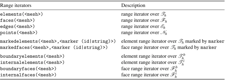
FEEL++ uses GMSH, see [20], to generate meshes in all 3 dimensions with 16kgeo65 ford=2 and 16
kgeo64 ford =3. The listing below and the resulting Figure1 forkgeo=1,2,3,4 illustrate the flexibility of FEEL++ regarding mesh handling.
t y p e d e f Mesh < Simplex <3 ,kgeo,3 > > m e s h _ t y p e ; // g e n e r a t e the m e s h of the s p h e r e u s i n g G m s h a u t o m e s h = c r e a t e G M s h M e s h ( _ m e s h =new m e s h _ t y p e ,
_ d e s c = d o m a i n ( _ s h a p e = " e l l i p s o i d " , _ d i m = 3 ) ) ;
// g e n e r a t e a f u n c t i o n s p a c e , see n e x t s e c t i o n
F u n c t i o n S p a c e < m e s h _ t y p e , bases < L a g r a n g e <kgeo> > > X h _ t y p e ; a u t o Xh = X h _ t y p e :: New ( m e s h );
// b u i l d the L a g r a n g e i n t e r p o l a n t u of d e g r e e kgeo of cos(5x)sin(5y)
a u t o u = p r o j e c t( _ s p a c e = Xh , _ r a n g e = e l e m e n t s ( m e s h ) , _ e x p r =cos(5x)sin(5y) );
// e x p o r t f u n c t i o n to g m s h the m e s h and u for h i g h o r d e r v i s u a l i s a t i o n // g m s h r e q u i r e s t h a t we use i s o p a r a m e t r i c e l e m e n t s
e x p o r t e r ( _ f o r m a t = gmsh , _ m e s h = mesh ,
_ n a m e = " h o _ s p h e r e " ). add ( _ d a t a = u , _ n a m e = " u " );
Finally the mesh data structure of topological dimension d allows to easily extract submeshes of topological dimension d andd−1. For example, the methods exposed in section5 use the extraction of trace meshes as follows:
// T r a c e m e s h c o m p o s e d of all b o u n d a r y f a c e s f r o m ’ m e s h ’ a u t o t r a c e _ m e s h = mesh - > t r a c e ( b o u n d a r y f a c e s ( m e s h ));
2http://www.boost.org/libs/multi_index/doc/index.html
3
http://www.boost.org/libs/range/index.html
// m e s h of f a c e s m a r k e d G a m m a in ’ m e s h ’
a u t o G a m m a _ m e s h = mesh - > t r a c e ( m a r k e d f a c e s ( mesh , " G a m m a " ));
Figure 1. Sphere discretized with 31 elements. Visualization of a function in Gmsh using tetrahedral elements of orderN=1,2,3,4.
3.2.
Algebraic representations
Algebraic representations are handled using a so-calledbackend which is a wrapper class that encapsulates several linear, nonlinear and eigenvalue algorithms as well as data structures like vectors and matrices. It provides all the algebraic data structure behind function spaces, operators and forms (see the following sections). In the case of linear functionals (also called linear forms or 1-forms), the representation is a vector and, in the case of linear operators and bilinear forms, the representation is a matrix.
Thebackendabstraction allows to write code that is independent of the libraries used in the assembly process or to solve the linear systems involved, thus hiding all the details of that algebraic part under the hood of the backend. Once a backend is set, the user can create in a transparent way vectors and matrices to be used during the assembly process, as is it shown is the following listing.
// a l l o c a t e s a s p a r s e m a t r i x b a s e d on the d e g r e e s of f r e e d o m of the // t r i a l f u n c t i o n s s p a c e Xh and the t e s t f u n c t i o n s s p a c e Vh
a u t o A = backend - > n e w M a t r i x ( _ t r i a l = Xh , _ t e s t = Vh );
// a l l o c a t e s a v e c t o r b a s e d on the d e g r e e s of f r e e d o m of the // t e s t f u n c t i o n s s p a c e Vh
a u t o b = backend - > n e w V e c t o r ( _ t e s t = Vh );
There are two available backends that provide an interface toPETSc/SLEPc, see [3–5,25], andTrilinos, see [26–29]. The user can choose any of them, bearing in mind the tools and features available in each, such as parallelism, direct or iterative linear system solvers or preconditioners for these systems. Once a backend is defined, sayBackend<Trilinos>, the user is free to manipulate objects such as vectors and matrices (from the
Epetraclass, in this case), using most of the algebraic operations attainable from the original library. The backend
also provides interfaces to linear system solvers (direct or iterative, with or without a preconditioner). The syntax for this function is illustrated in the next listing. Similar interfaces exist for non-linear and standard/generalized eigenvalue solvers.
// s o l v e the l i n e a r s y s t e m Au = F
b a c k e n d - > s o l v e ( _ m a t r i x = A , _ s o l u t i o n = u , _ r h s = F );
3.3.
Function Spaces and Functions
We now turn to the next crucial mathematical ingredient: the function space, whose definition depends onΩh — or more precisely its partitioningTh— and the choice of basis function. Function spaces in FEEL++ follow the same definition, see listing1, and FEEL++ provides support for continuous and discontinuous Galerkin methods and in particular approximations inL2,H1-conforming andH1-nonconforming,H2,H(div)andH(curl)4.
Listing 1. FunctionSpace
// s p a c e of c o n t i n u o u s p i e c e w i s e // P3 f u n c t i o n s d e f i n e d on a m e s h
4At the time of writing,H2,H(div)andH(curl)approximations are in experimental support.
// of o r d e r 2 t r i a n g l e s in 3 D
F u n c t i o n S p a c e < Mesh < Simplex <2 ,2 ,3 > , bases < L a g r a n g e <3 > > > Xh ;
TheFunctionSpaceclass (i) constructs the table of degrees of freedom which maps local (elementwise) degrees
of freedom to the global ones with respect to the geometrical entities, (ii) embeds the definition of the elements of the function space allowing for a tight coupling between the elements and their function spaces, (iii) stores an interpolation data structure (e.g. region tree) for rapid localisation of point sets (determining in which element they reside).
We introduce the following spaces
Wh={vh∈L2(Ωh): ∀K∈Th,vh|K∈PK},
Vh=Wh∩C0(Ωh) ={vh∈Wh: ∀F∈Fhi {{vh}}F=0}
Hh=Wh∩C1(Ωh) ={vh∈Wh: ∀F∈Fhi {{vh}}F={{∇vh}}F=0} CRh={vh∈L2(Ωh): ∀K∈Th,vh|K∈P1;∀F∈Fhi
Z
F{{
vh}}=0}
RaTuh={vh∈L2(Ωh): ∀K∈Th,vh|K∈span
1,x,y,x2−y2 ;∀F∈Fhi
Z
F{{
vh}}=0}
RTh={vh∈[L2(Ωh)]d: ∀K∈Th,vh|K∈RTk;∀F∈Fhi {{vh·n}}F=0} Nh={vh∈[L2(Ωh)]d: ∀K∈Th,vh|K∈Nk;∀F∈Fhi {{vh×n}}F=0}
(1)
whereRTk andNk are respectively the Raviart-Thomas and N´ed´elec finite elements of degreek. The table2 summarizes the supported approximation spaces.
Continuous Solution Space Discrete Approximation Space Basis Order Dimension
L2 Wh
Lagrange
any 1,2,3
Legendre Dubiner
H1-conforming Vh
Lagrange
any 1,2,3
Legendre boundary adapted Dubiner boundary adapted
H1-nonconforming CRh Crouzeix-Raviart 1 2,3
RaTuh Rannacher-Turek 2 2
H(div)-conforming RTh Raviart-Thomas any 2,3
H(curl)-conforming Nh N´ed´elec first kind any 2,3
H2-conforming Hh Hermite >2 1,2,3
Table 2. FEEL++ approximations spaces
The Legendre and Dubiner basis yield implicitly discontinuous approximations, the Legendre and Dubiner boundary adapted basis, see [32], were designed to handle continuous approximations whereas the Lagrange basis can yield either discontinuous or continuous (default behavior) approximations.RThandNhare implicitly spaces of vectorial functionsfs.t.f:Ωh⊂Rd7→Rd. As to the other basis functions, i.e. Lagrange, Legrendre, Dubiner, etc., they are parametrized by their values namelyScalar,VectorialorMatricial. Note thatFunctionSpace
handles also products of function spaces. This is very powerful to describe complex multiphysics problems when coupled with operators, functionals and forms described in the next section. Extracting subspaces or component spaces are part of the interface.
// c o n t i n u o u s p i e c e w i s e P3 // a p p r o x i m a t i o n s
F u n c t i o n S p a c e < Mesh < Simplex <2 > > , bases < L a g r a n g e <3 , Scalar ,
C o n t i n u o u s > > > P 3 c h ;
// d i s c o n t i n u o u s p i e c e w i s e P3
// a p p r o x i m a t i o n s
F u n c t i o n S p a c e < Mesh < Simplex <2 > > , bases < L a g r a n g e <3 , Scalar ,
D i s c o n t i n u o u s > > > P 3 d h ;
// m i x e d ( P2 v e c t o r i a l , P1 scalar , // P1 S c a l a r ) a p p r o x i m a t i o n
F u n c t i o n S p a c e < Mesh < Simplex <2>>, bases < L a g r a n g e <2 , V e c t o r i a l > ,
L a g r a n g e <1 , Scalar > ,
L a g r a n g e <1 , S c a l a r>>> P 2 P 1 P 1 ;
The most important feature inFunctionSpaceis that it embeds the definition of element which allows for the strict definition of an Element of aFunctionSpaceand thus ensures the correctness of the code. An element has its representation as a vector — also in the case of product of multiple spaces. — The vector representation is parametrized by one of the linear algebra backends presented in section3.2. Other supported operations are interpolation and extraction of components — be it a product of function spaces element or a vectorial/matricial element, — see listing3.3.
F u n c t i o n S p a c e < Mesh < Simplex <2 > > ,
bases < L a g r a n g e <3 , Scalar , C o n t i n u o u s > > > P 3 c h ;
// get an e l e m e n t f r o m P 3 c h a u t o u = P 3 c h . e l e m e n t ();
F u n c t i o n S p a c e < Mesh < Simplex <2 > > ,
bases < L a g r a n g e <2 , V e c t o r i a l > , L a g r a n g e <1 , Scalar > , L a g r a n g e <1 , Scalar > > > P 2 P 1 P 1 ;
a u t o U = P 2 P 1 P 1 . e l e m e n t ();
// V i e w s : c h a n g i n g a v i e w c h a n g e s U and v i c e v e r s a // v i e w on e l e m e n t a s s o c i a t e d to P2
a u t o u = U . element <0 >();
// e x t r a c t v i e w of f i r s t c o m p o n e n t a u t o ux = u . c o m p ( X );
// v i e w on e l e m e n t a s s o c i a t e d to 1 st P1 a u t o p = U . element <1 >();
// v i e w on e l e m e n t a s s o c i a t e d to 2 nd P1 a u t o q = U . element <2 >();
Finally FEEL++ provides the Lagrange, IcLAG,h ,IdLAG,h , Crouzeix-Raviart, IhCR, Raviart-Thomas, IhRT and N´ed´elec,IhNglobal interpolation operators. In abstract form, they read
I :X3v7→
dimX
∑
i=1`i(v)φi (2)
whereXis the infinite dimensional space,(`i)i=1,...,dimXare the linear forms and(φi)i=1...dimXthe basis function associated with the various approximations in table2.
3.4.
Functionals, Operators and Forms
We now introduce the necessary functional vocabulary, namely (i) functionals,`:X7→R, (ii) operators,A : X7→Yand (iii) bilinear forms,a:X×Y7→R. Note that for a bilinear forma:X×Y7→Rthere exists a unique operatorA :X7→Y0s.t.a(x,y) =hAx,yiwhereh·,·idenotes the duality product. TheC++counterpart of these mathematical objects follows closely their mathematical analog: they are template classes with arguments being the space (or product of spaces) they take as input and provide an interface to apply them on elements of the domain space. For operators, we can also apply their inverse to the elements of the image space. In the linear case, we provide also an algebraic representation : a vector for linear functionals or forms and a matrix for linear operators and bilinear forms — matrix- and vector-free representations are possible too. — The listing below exercises
a u t o Xh = Xh_ t y p e :: New ( m e s h ); Vh = Vh_ t y p e :: New ( m e s h ); a u t o u = Xh- > e l e m e n t (); a u t o v = Vh- > e l e m e n t ();
// o p e r a t o r T:Xh→Vh0
a u t o T = o p L i n e a r ( _ d o m a i n S p a c e =Xh, _ i m a g e S p a c e = d u a l (Vh) [ , _ b a c k e n d = b a c k e n d ] );
// d e f i n i t i o n of T , see eg s e c t i o n 4
T = i n t e g r a t e( _ r a n g e = e l e m e n t s ( m e s h ) , _ e x p r =g r a d t( u )* t r a n s (g r a d( v ) ) ) ;
// l i n e a r f u n c t i o n a l f:Vh→R
// f is a l i n e a r f o r m
a u t o f = T . a p p l y ( u ); f . a p p l y ( v );
// or e q u i v a l e n t l y
a u t o f = f u n L i n e a r ( _ d o m a i n S p a c e =Vh [ , _ b a c k e n d = b a c k e n d ] ); f = T . a p p l y ( u ); f . a p p l y ( v ) ;
// a is a b i l i n e a r form ,
a u t o A = backend - > n e w M a t r i x ( _ t e s t =Xh, _ t r i a l =Xh );
a u t o a = f o r m 2( _ t e s t =Xh, _ t r i a l =Xh, _ m a t r i x = A );
// d e f i n i t i o n of a , see e . g . s e c t i o n 4
a = i n t e g r a t e( _ r a n g e = e l e m e n t s ( m e s h ) , _ e x p r =idt( u )*id( v ));
// b is a l i n e a r form ,
a u t o B = backend - > n e w V e c t o r ( _ t e s t =Xh );
a u t o b = f o r m 1( _ t e s t =Xh, _ v e c t o r = B );
// d e f i n i t i o n of b , see e . g . s e c t i o n 4
b = i n t e g r a t e( _ r a n g e = e l e m e n t s ( m e s h ) , _ e x p r =id( v ));
FEEL++ implements currently the following operators (i) interpolation operator, (ii) the lift and trace operators, and (iii) the projection operators (L2,H1,H(div),H(curl),...). We describe briefly the interpolation operator which is used later in this text. Note that the lift and trace operators are used also in some examples in section5.
The interpolation operator,I :X−→Y whereY is a nodal basis andI(v),v∈X is the interpolant ofv∈Y, defined in the previous section. It is based on two fundamental tools: a localisation tool using a kd-tree data structure for fast localisation and the inverse geometrical transformation. This is a crucial tool for all advanced numerical methods presented later in this paper in sections5and6.
Listing 2. Interpolation operator
a u t o Xh = Xh_ t y p e :: New ( m e s h ); Vh = Vh_ t y p e :: New ( m e s h );
a u t o u = Xh- > e l e m e n t (); a u t o v = Vh- > e l e m e n t ();
// o p e r a t o r I:Xh→Vh
a u t o I = o p I n t e r p o l a t i o n ( _ d o m a i n S p a c e =Xh, _ i m a g e S p a c e =Vh [ , _ b a c k e n d = b a c k e n d ] );
// c o m p u t e v the i n t e r p o l a n t of u in Vh
v = I ( u );
4. A V
ARIATIONALF
ORMULATIONL
ANGUAGEE
MBEDDED INC
++The language has a variety of keywords — see appendixAfor an exhaustive list — that implement (i) access to geometrical data structure, e.g. exterior normal to the face of an element, (ii) standard mathematical functions and logical relations, (iii) operations related with the function spaces, such as element evaluation or differentiation, (iv) numerical integration. These keywords, with the help of algebraic operations such as sum, multiplication, division, etc, allow to build expressions which are used to define mathematical expressions then used by various objects such as forms or operators.
Some keywords show a common pattern in their nomenclature: for instance, the basic expressions id(p), grad(p),jump(p)ordiv(p)represent the evaluation, gradient, jump across a face or divergence of a test function, while the addition oftat the end of such expressions (idt(p),gradt(p),jumpt(p)ordivt(p)) represents the same operators, but now concerning trial functions. Therefore, ifpandqbelong to the same function space, the construction of a bilinear form associated with the expressionidt(p)*id(q) will result in the assembly of the associated mass matrix. However, adding avat the end of the keywords, allows to perform evaluation of the operator applied to the argument, ie,idv(p),gradv(p),jumpv(p)ordivv(p)evaluate respectively the gradient of
p, the jump ofpacross faces or the divergence ofp.
Finally FEEL++ supports scalar, vectorial and matricial operations in expressions. Indeed theC++operators follow the same rank semantics of their mathematical counterparts, see appendixA. Listing3displays aC++code solving the linear elasticity equations, notice how the vectorial notations make it easy to express the variational formulation.
Often it is the case that we must integrate function space elements or basis functions (trial or test functions) that are defined on a mesh which is different from the integration mesh, see e.g. the mortar method in section5.2or the Fat Boundary Method in section6. Such a case is detected automatically and the interpolation procedure is called in the background of the integration or projection processes automatically to handle the necessary information transfer. All possible cases are actually handled by FEEL++.
4.1.
Integration
Integration is of course a fundamental tool in FEEL++. It is handled through the keywordintegrateand is used to define forms, functionals and operators or just to compute integrals. It provides an extremely flexible and versatile interface in all these contexts:
i n t e g r a t e( _ r a n g e = < m e s h r a n g e i t e r a t o r s > , // i n t e g r a t i o n d o m a i n
_ e x p r = < e x p r e s s i o n to i n t e g r a t e> , // i n t e g r a n d
_ q u a d = _Q < p o l y n o m i a l o r d e r to i n t e g r a t e exactly >() , // q u a d r a t u r e
... // o t h e r p a r a m e t e r s are a v a i l a b l e but not n e c e s s a r y h e r e );
The parameters_range(domain of integration) and_expr(integrand) are required while_quadis optional. In-deed, by default, the DSEL computes an approximation of the polynomial order of the integrand and selects the quadrature that integrates it exactly (if the integrand is polynomial then the integration is exact). If this is not satisfactory then the user selects his own quadrature. Multipleintegratekeywords can be accumulated using the+operator and returns an object which is handled automatically by forms, functionals and operators. There are two particular flavors: (i) integral evaluation which requires to use theevaluate()member function of the object returned byintegrate()(ii) elementwise integral evaluation which requires to use of thebroken(<space>)
member function to return an element of<space>(typically a space of piecewise constant functions) containing the resulting integral computations.
t y p e d e f F u n c t i o n S p a c e < Mesh < Simplex <3 > ,
bases < L a g r a n g e <0 , Scalar , D i s c o n t i n u o u s > > > P 0 h _ t y p e ; a u t o P0h = P 0 h _ t y p e :: New ( m e s h )
// e v a l u a t e R
Ωhsinx=∑K∈Th
R Ksinx
a u t o v = i n t e g r a t e( _ r a n g e = e l e m e n t s ( m e s h ) , _ e x p r =sin( Px()) ). e v a l u a t e ();
// s t o r e for all K∈Th, R
Ksinx in p0 [ιK] w h e r e ιK is the
// i n d e x of e l e m e n t K
a u t o p0 = i n t e g r a t e( _ r a n g e = e l e m e n t s ( m e s h ) , _ e x p r =sin( Px()) ). b r o k e n ( P0h ); for( a u t o ιK : m e s h . e l e m e n t s () ) {
// p r i n t the e l e m e n t w i s e i n t e g r a l s
std :: c o u t < < " p0 [ " < < ιK < < " ]= " < < p [ιK] < < " \ n " ;
}
Note that there is a special keyword in the context of bilinear forms and linear operators used conjointly with integrate, it isonwhich allows to eliminate Dirichlet “degrees of freedom”.
4.2.
Projection
Another important keyword isprojectwhich allows to compute the interpolant of an expression with respect to a nodal function space over a part of the mesh or the whole mesh. The interface is as follows
p r o j e c t( _ s p a c e = < n o d a l f u n c t i o n s p a c e in w h i c h the i n t e r p o l a n t lives > _ r a n g e = < d o m a i n r a n g e i t e r a t o r s > ,
_ e x p r = < e x p r e s s i o n to be i n t e r p o l a t e d > , . . . . )
Here are some examples
t y p e d e f F u n c t i o n S p a c e < Mesh < Simplex <d> ,
bases < L a g r a n g e <1 , V e c t o r i a l > > > X h v _ t y p e ; a u t o Xhv = X h v _ t y p e :: New ( m e s h );
// b u i l d a p i e c e w i s e P1 v e c t o r i a l f u n c t i o n in Xhv c o n t a i n i n g the // c o o r d i n a t e s of the v e r t i c e s the m e s h .
a u t o c o o r d = p r o j e c t( _ s p a c e = Xhv , _ r a n g e = e l e m e n t s ( m e s h ) , _ e x p r =P() );
// c o m p u t e the x d e r i v a t i v e of the c o o r d f u n c t i o n
a u t o d x _ c o o r d = p r o j e c t( _ s p a c e = Xhv , _ r a n g e = e l e m e n t s ( m e s h ) , _ e x p r =dxv( c o o r d ) ); a u t o d y _ c o o r d = p r o j e c t( _ s p a c e = Xhv , _ r a n g e = e l e m e n t s ( m e s h ) , _ e x p r = dyv ( c o o r d ) );
4.3.
A wrap up example
To finish, we present an example in linear elasticity which is dimension independent and takes only few lines of code to express.
Listing 3. Solving a linear elasticity problem on a campled beam
F u n c t i o n S p a c e < m e s h _ t y p e , bases < L a g r a n g e <1 , V e c t o r i a l>>> s p a c e _ t y p e ; a u t o Xh = s p a c e _ t y p e :: New ( m e s h );
a u t o u = Xh - > e l e m e n t (); v = Xh - > e l e m e n t ();
// s t r a i n t e n s o r 0.5∗(∇u+∇uT)
a u t o F = backend - > n e w V e c t o r ( Xh );
a u t o f o r c e =p r o j e c t( _ s p a c e = Xh , _ r a n g e = m a r k e d f a c e ( mesh , " f o r c e Z " ) , _ e x p r = vec (0 ,0 , -1) );
f o r m 1( _ t e s t = Xh , _ v e c t o r = F ) = i n t e g r a t e( m a r k e d f a c e s ( mesh , " F o r c e Z " ) , t r a n s (idv( f o r c e ))*id( v ) ); a u t o d e f t = sym (g r a d t( u ));
a u t o def = sym (g r a d( u ));
a u t o l a m b d a =... , mu = . . . . ; // L a m e c o e f f i c i e n t s a u t o D = backend - > n e w M a t r i x ( Xh , Xh );
f o r m 2( _ t e s t = Xh , _ t r i a l = Xh , _ m a t r i x = D ) = i n t e g r a t e( e l e m e n t s ( m e s h ) ,
l a m b d a *d i v t( u )*div( v ) + 2* mu * t r a c e ( t r a n s ( d e f t )* def ))+
on( m a r k e d f a c e s ( mesh , " c l a m p e d " ) , u , F , 0* one ( ) ) ;
// s o l v e
backend - > s o l v e ( _ m a t r i x = D , _ s o l u t i o n = u , _ r h s = F );
// a p p l y d i s p l a c e m e n t to the m e s h
m o v e m e s h ( mesh , u );
5. D
OMAIN DECOMPOSITION METHODSWe now turn to advanced numerical methods to exercise our framework and show that the embedding language (C++) goes little in the way of the expressivity and closeness to the mathematical language. We first investigate domain decomposition methods such as overlapping and nonoverlapping Schwartz methods, mortar and three fields methods. Domain decomposition methods provide techniques to find the solution of problems defined over domain from the solution of related problems defined on subdomains. They are also used in coupling discretisation methods or models and are suited for parallel computing.
Throughout this section we denoteΩa domain ofRd, d =1,2,3,and∂Ω its boundary. We look foru the solution of the problem:
Lu= f in Ω
u=g on ∂Ω (3)
whereL is a partial differential operator, and the functions f andg are given. For the sake of exposition we refer to the case of a domainΩpartitioned into two subdomainsΩ1andΩ2such thatΩ=Ω1∪Ω2. We denote Γ1:=∂Ω1∩Ω2andΓ2:=∂Ω2∩Ω1, in the case of two overlapping subdomains, andΓ:=∂Ω1∩∂Ω2, in the case of two nonoverlapping subdomains. The norm ofH1(Φ)will be denoted byk·k1,Φ, whilek·k0,Φwill indicate the
norm ofL2(Φ)for all nonempty subsetΦ⊆Ω.
5.1.
Overlapping and nonoverlapping Schwartz methods
First we are interested in the overlapping and nonoverlapping Schwartz methods [47]. The overlapping mul-tiplicative Schwartz algorithm with Dirichlet interface conditions at(k+1)th iteration, k≥0, is given by (4) whereu02is known onΓ1. The additive version of this algorithm is obtained by changing the interface condition
uk2+1=uk1+1on the second subdomainΩ2touk2+1=uk1in the second system of (4).
Luk1+1=f in Ω1
uk1+1=g on ∂Ω1\Γ1
uk1+1=uk2 on Γ1
Luk2+1=f in Ω2
uk2+1=g on ∂Ω2\Γ2
uk2+1=uk1+1 on Γ2
(4)
The nonoverlapping Schwartz algorithm with Dirichlet and Neumann interface conditions at(k+1)thiteration, k≥0, are given by
Luk1+1=f in Ω1
uk1+1=g on ∂Ω1\Γ
uk1+1=λk on Γ
Luk2+1= f in Ω2
uk2+1=g on ∂Ω2\Γ ∂uk2+1
∂n =
∂uk1+1
∂n on Γ
(5)
Listing 4Fixed point algorithm using Aitken acceleration for (4) and (5)
e n u m D D M e t h o d { DD = 0 ,/* D i r i c h l e t - D i r i c h l e t */
DN = 1 /* D i r i c h l e t - N e u m a n n */ }; a u t o a c c e l = a i t k e n ( _ s p a c e = Xh2 );
a c c e l . i n i t i a l i z e ( _ r e s i d u a l = r e s i d u a l , _ c u r r e n t E l t = l a m b d a ); d o u b l e m a x I t e r a t i o n = 20;
w h i l e( ! a c c e l . i s F i n i s h e d () &&
a c c e l . n I t e r a t i o n s () < m a x I t e r a t i o n ) {
// c a l l the l o c a l P r o b l e m on the f i r s t s u b d o m a i n Ω1 l o c a l P r o b l e m ( u1 , idv( u2 ) , D D M e t h o d :: DD );
l a m b d a = u2 ;
// c a l l the l o c a l P r o b l e m on the f i r s t s u b d o m a i n Ω2 if( d d m e t h o d = D D M e t h o d :: DD )
l o c a l P r o b l e m ( u2 , idv( u1 ) , D D M e t h o d :: DD ); e l s e
l o c a l P r o b l e m ( u2 , g r a d v( u1 )*N() , D D M e t h o d :: DN ); r e s i d u a l = u2 - l a m b d a ;
u2 = a c c e l . a p p l y ( _ r e s i d u a l = r e s i d u a l , _ c u r r e n t E l t = u2 ); ++ a c c e l ;
}
whereλk+1:=θuk2+|1
Γ + (1−θ)λ
k,
θbeing a positive acceleration parameter which can be computed for example
by an Aitken procedure, see listing5, andλ0is given onΓ. The additive Schwartz method requires generally more iterations than the multiplicative method and is naturally parallelizable. The generalization of these algorithms to many subdomains is immediate.
The numerical solutions in Figures2(b)-2(d)correspond to the partition ofΩinto two subdomainsΩ1andΩ2 and the following configuration: (i)g(x,y) =sin(πx)cos(πy)is the exact solution (ii) f(x,y) =2π2gis the right hand side of the equation (iii) we useP2Lagrange approximation (iv) we use the maximal number of iteration equal to 10. Table 3 summarizes TheL2 andH1 errors for both problems studied. Finally we present a 3D nonoverlapping Schwartz example using the same code in Figure3.
ku1−gk0,Ω
1 ku2−gk0,Ω2 ku1−gk1,Ω1 ku2−gk1,Ω2
With overlap 2.52e-8 2.16e-8 4.07e-6 3.89e-6
Without overlap 1.37e-9 2.04e-8 1.32e-6 6.71e-6
Table 3. Numerical results for Schwartz methods
Ω1
Ω2
Ω
1∩
Ω
2
(a) Geometry (b) Solution
1
2
(c) Geometry (d) Solution
Figure 2. Overlapping and nonoverlapping cases in 2D
5.2.
Mortar domain decomposition method
Consider the problem (3) whereL:=−∆and homogeneous Dirichlet boundary conditions. We assume thatΩ is partitioned into two nonoverlapping subdomains and it is ad-dimensional domain (d=2,3), with a Lipschitz boundary∂Ω. We also assume that f belongs toL2(Ω). The main idea of this method is to enforce the weak
Listing 5Local problems for (4) and (5)
t e m p l a t e< Expr > v o i d l o c a l P r o b l e m ( e l e m e n t _ t y p e & u , E x p r expr , D D M e t h o d d d m e t h o d ) {
a u t o Xh = u . f u n c t i o n S p a c e (); a u t o m e s h = Xh - > m e s h (); a u t o v = Xh - > e l e m e n t ();
a u t o F = M _ b a c k e n d - > n e w V e c t o r ( Xh );
a u t o A = M _ b a c k e n d - > n e w M a t r i x ( Xh , Xh );
// A s s e m b l y of the r i g h t h a n d s i d e Z
Ω f v
f o r m 1( _ t e s t = Xh , _ v e c t o r = F ) = i n t e g r a t e( e l e m e n t s ( m e s h ) , f *id( v ) );
// A s s e m b l y of the l e f t h a n d s i d e Z
Ω
∇u·∇v f o r m 2( _ t e s t = Xh , _ t r i a l = Xh , _ m a t r i x = A ) =
i n t e g r a t e( e l e m e n t s ( m e s h ) , g r a d t( u )* t r a n s (g r a d( v )) );
// Add N e u m a n n c o n t r i b u t i o n if ( d d m e t h o d == D D M e t h o d :: DN )
f o r m 1( _ t e s t = Xh , _ v e c t o r = F ) += i n t e g r a t e( m a r k e d f a c e s ( mesh , " I n t e r f a c e " ) , _ e x p r = e x p r *id( v ));
e l s e if( d d m e t h o d == D D M e t h o d :: DD )
f o r m 2( Xh , Xh , A ) += on( m a r k e d f a c e s ( mesh , " I n t e r f a c e " ) , u , F , e x p r );
// A p p l y the D i r i c h l e t b o u n d a r y c o n d i t i o n s
f o r m 2( Xh , Xh , A ) += on( m a r k e d f a c e s ( mesh , " D i r i c h l e t " ) , u , F , g );
// A p p l y the D i r i c h l e t i n t e r f a c e c o n d i t i o n s // s o l v e the l i n e a r s y s t e m Au=F
M _ b a c k e n d - > s o l v e ( _ m a t r i x = A , _ s o l u t i o n = u , _ r h s = F ); }
(a) Geometry (b) Solution
Figure 3. An example of nonoverlapping Schwartz method in 3D
continuity between the solutions on each subdomain. This is achieved by introducing a Lagrange multiplier corresponding to this connection constraint [7]. Problem (3) is equivalent to findingu∈H01(Ω)such that
J(u) = min v∈H01(Ω)
J(v), J(v) =1 2
Z
Ω| ∇v|2−
Z
Ω
f v. We denote byJi(v):= 1 2
Z
Ωi
|∇vi|2−
Z
Ω
f vi i=1,2.
The problem is now equivalent to find(u1,u2)∈Hsuch as
J1(u1) +J2(u2) = min (v1,v2)∈H
J1(v1) +J2(v2),H= n
(v1,v2)∈H1(Ω1)×H1(Ω2): vi=0 on∂Ωi\Γ,v1=v2onΓ o
.
We define the Lagrangian byL(v1,v2;µ):=J1(v1) +J2(v2) +
Z
Γ
µ(v1−v2)and we search for the saddle point
solution(u1,u2,λ)such that
L(u1,u2;µ)≤L(u1,u2;λ)≤L(v1,v2;λ), ∀(v1,v2)∈V1h×V2h ∀µ∈Wh. (6)
Let us denote byVihthe finite element approximation space onΩi, of basis(ψi,j)j=1,···Ni,i=1,2,and byWhthat ofΓ, of basis(φk)k=1,···K.
Then the saddle point(u1,u2,λ)can be approximated by the solution of the following discrete system
A1U1,h+Bt1Lh=f1
A2U2,h−Bt2Lh=f2
B1U1,h−B2U2,h=0
where
(Ai)jl=
Z
Ωi
∇ψi j·∇ψil j,l=1,···,Ni
(Bi)k j=
Z
Γ
ψi jφk k=1,···,K, j=1,···,Ni
(fi)j=
Z
Ωi
fψi j j=1,···,Ni
(7)
andU1,h,U2,handLhcollect the degrees of freedom ofu1,h,u2,handλh, approximations tou1,u2andλ. In Listing6we display the terms corresponding to the jump matricesB1andB2in equation (7).
Listing 6Jump terms in the global matrix
// f u n c t i o n s p a c e s and s o m e a s s o c i a t e d e l e m e n t s ( f u n c t i o n s ) for Ω1 and Ω2 a u t o Xh1 = s p a c e 1 _ t y p e :: New ( m e s h 1 );
a u t o u1 = Xh1 - > e l e m e n t ();
a u t o Xh2 = s p a c e 2 _ t y p e :: New ( m e s h 2 ); a u t o u2 = Xh2 - > e l e m e n t ();
// t r a c e m e s h and L a g r a n g e m u l t i p l i e r s p a c e and a s s o c i a t e d f u n c t i o n for Γ
a u t o Lh = l a g m u l t _ s p a c e _ t y p e :: New ( mesh1 - > t r a c e ( m a r k e d f a c e s ( mesh1 , g a m m a ) )); a u t o mu = Lh - > e l e m e n t ();
// a s s e m b l y of j u m p m a t r i c e s B1 and B2
a u t o B1 = M _ b a c k e n d - > n e w M a t r i x ( _ t r i a l = Xh1 , _ t e s t = Lh );
f o r m 2( _ t r i a l = Xh1 , _ t e s t = Lh , _ m a t r i x = B1 ) =
i n t e g r a t e( e l e m e n t s ( Lh - > m e s h ()) , idt( u1 )*id( mu ) );
a u t o B2 = M _ b a c k e n d - > n e w M a t r i x ( _ t r i a l = Xh2 , _ t e s t = Lh );
f o r m 2( _ t r i a l = Xh2 , _ t e s t = Lh , _ m a t r i x = B2 ) =
i n t e g r a t e( e l e m e n t s ( Lh - > m e s h ()) , idt( u2 )*id( mu ) );
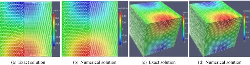
Figures4(b)and4(d)correspond to the solution of (7) whenΩ is partitioned into two nonoverlapping sub-domainsΩ1andΩ2and the following configurations are set: (i)g(x,y) =sin(πx)cos(πy)is the exact solution (ii) f(x,y) =2π2gis the right hand side of the equation (iii) we useP2andP3approximations, respectively, inΩ1 andΩ2(iv)hΩ1=0.015 andhΩ2=0.04 in 2D (v)hΩ1=0.075 andhΩ2 =0.05 in 3D.
(a) Exact solution (b) Numerical solution (c) Exact solution (d) Numerical solution
Figure 4. Exact and Numerical solutions in 2D and 3D for mortar method
The numerical solutions 5(b)and 5(d)correspond to the same configuration used previously but we change the polynomial orders and mesh sizes as (i)P7andP6approximations, respectively, inΩ1andΩ2,hΩ1 =0.1 and
hΩ2 =0.15 in 2D (ii)P3andP4approximations, respectively, inΩ1andΩ2,hΩ1=0.75 andhΩ2 =0.5 in 3D.
Table4summarizes several error quantities for both problems studied and the global solutionuhdefined onΩas uh=u1,honΩ1anduh=u2,honΩ2.
(a) Exact solution (b) Numerical solution (c) Exact solution (d) Numerical solution
Figure 5. Exact and Numerical solutions in 2D and 3D for mortar method using higher order approximations
P-orders ku1,h−gk0,Ω1 ku2,h−gk0,Ω2 ku1,h−gk1,Ω1 ku2,h−gk1,Ω2 kλh−gk0,Γ kuh−gk1,Ω
2D case P2−P3 3.39695e-08 1.88289e-08 8.67241e-06 2.2959e-06 6.69075e-09 8.97116e-06
P7−P6 1.13996e-09 7.35774e-10 2.92219e-07 1.15223e-07 2.29634e-11 3.14115e-07
3D case P2−P3 8.74556e-06 8.40938e-06 1.17e-04 9.72e-05 1.52e-05 2.17e-04
P3−P4 9.28974e-07 8.97491e-07 3.55e-05 3.50e-05 1.03e-07 4.99e-05
Table 4. Numerical results for mortar methods in 2D and 3D
5.3.
Three fields domain decomposition method
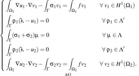
The weak formulation of (3) reads: findu∈H01(Ω)such thatR
Ω∇u·∇v= R
Ωf v, ∀v∈H 1
0(Ω). Denoting byui the restriction of the solution u toΩi,i=1,2,the interface conditions onΓare∂u1/∂n=∂u2/∂n andu1=u2onΓ. The three fields formulation [11] rewrites the original problem by relaxing the continuity requirements on both
uand∂u/∂n, at the expense of introducing two Lagrange multipliers for each subdomain. The new weak formu-lation allows independent approximations within the subdomains, including the possibility of using different meth-ods and different meshes on both subdomains. First for all, let us defineΛ:=
n
η∈H1/2(Γ)|η=v|Γ for a suitablev∈H1(Ω) o
the trace space andΛ0its dual. The finite dimensional approximation of (8) can be devised by selecting suitable subspacesVi,hofVi:=H1(Ωi),Ξi,hofΛ0andΛhofΛ. We denote by(ψi,j)j=1,···Nia basis ofVi,h,(χi,k)k=1,···Kithat ofΛ0and(φk)k=1,···K that ofΛ. In the following formulation,σiis the Lagrange multiplier that is used to ‘glue’ the value ofuiandλ onΓ, i=1,2.As a matter of fact, the following equivalence result holds between the weak form of the unsplit problem (3) and the problem with Lagrange multipliers. The three fields formulation is given by: fori=1,2 findui∈Vi:=H1(Ωi),σi∈Λ0,λ∈Λsuch that
Z
Ω1
∇u1·∇v1−
Z
Γ σ1v1=
Z
Ω1
f v1 ∀v1∈H1(Ω1)
Z
Γ
ρ1(λ−u1) =0 ∀ρ1∈Λ0
Z
Γ
(σ1+σ2)µ=0 ∀µ∈Λ
Z
Γ
ρ2(λ−u2) =0 ∀ρ2∈Λ0
Z
Ω2
∇u2·∇v2−
Z
Γ σ2v2=
Z
Ω2
f v2 ∀v2∈H1(Ω2).
(8)
Problem (8) can be stated in algebraic form as
A1U1,h−Bt1S1,h =f1 −B1U1,h+Ct1Lh =0 C1S1,h+C2S2,h =0 −B2U2,h+Ct2Lh =0 A2U2,h−Bt2S2,h =f2
where
(Ai)jl=
Z
Ωi
∇ψi j∇ψil j,l=1,···,Ni
(Bi)k j=
Z
Γ
ψi jχi,k k=1,···,Ki, j=1,···,Ni
(Ci)k j=
Z
Γ
χi,jφk j=1,···,Ki, k=1,···,K
(fi)j=
Z
Ωi
fψi j j=1,···,Ni
(9)
andUi,h,Si,h,Lhcollect the degrees of freedom ofui,h,σσσi,handλh, approximations toui,σσσiandλ. In Listing7we display the terms corresponding to the jump matricesB1,C1,B2andC2in equation (9).
Listing 7Jump terms in the global matrix
// f u n c t i o n s p a c e s and s o m e a s s o c i a t e d e l e m e n t s ( f u n c t i o n s ) for Ω1 and Ω2 a u t o Xh1 = s p a c e 1 _ t y p e :: New ( m e s h 1 );
a u t o u1 = Xh1 - > e l e m e n t ();
a u t o Xh2 = s p a c e 2 _ t y p e :: New ( m e s h 2 ); a u t o u2 = Xh2 - > e l e m e n t ();
// t r a c e m e s h e s and L a g r a n g e m u l t i p l i e r s p a c e s and a s s o c i a t e d e l e m e n t s
a u t o Lh1 = l a g m u l t _ s p a c e 1 _ t y p e :: New ( mesh1 - > t r a c e ( m a r k e d f a c e s ( mesh1 , g a m m a ) ) ) ; a u t o mu1 = Lh1 - > e l e m e n t ();
a u t o Lh2 = l a g m u l t _ s p a c e 2 _ t y p e :: New ( mesh2 - > t r a c e ( m a r k e d f a c e s ( mesh2 , g a m m a ) ) ) ; a u t o mu2 = Lh2 - > e l e m e n t ();
a u t o Lh = i n t e r f a c e _ s p a c e _ t y p e :: New ( i n t e r f a c e _ m e s h ); a u t o mu = Lh - > e l e m e n t ();
// a s s e m b l y of j u m p m a t r i c e s B1 and B2
a u t o B1 = M _ b a c k e n d - > n e w M a t r i x ( _ t r i a l = Xh1 , _ t e s t = Lh1 );
f o r m 2( _ t r i a l = Xh1 , _ t e s t = Lh1 , _ m a t r i x = B1 ) =
i n t e g r a t e( e l e m e n t s ( Lh1 - > m e s h ()) , idt( u1 )*id( mu1 ) );
a u t o C1 = M _ b a c k e n d - > n e w M a t r i x ( Lh , Lh1 );
f o r m 2( _ t r i a l = Lh , _ t e s t = Lh1 , _ m a t r i x = C1 ) +=
i n t e g r a t e( e l e m e n t s ( Lh - > m e s h ()) , idt( mu )*id( mu1 ) );
a u t o B2 = M _ b a c k e n d - > n e w M a t r i x ( _ t r i a l = Xh2 , _ t e s t = Lh2 );
f o r m 2( _ t r i a l = Xh2 , _ t e s t = Lh2 , _ m a t r i x = B2 ) =
i n t e g r a t e( e l e m e n t s ( Lh2 - > m e s h ()) , idt( u2 )*id( mu2 ) );
a u t o C2 = M _ b a c k e n d - > n e w M a t r i x ( Lh , Lh2 );
f o r m 2( _ t r i a l = Lh , _ t e s t = Lh2 , _ m a t r i x = C2 ) +=
i n t e g r a t e( e l e m e n t s ( Lh - > m e s h ()) , idt( mu )*id( mu2 ) );
The following numerical solutions 6(b)and 6(d)correspond to partition ofΩinto two nonoverlapping subdo-mainsΩ1andΩ2and the following configurations (i)g(x,y) =sin(πx)cos(πy)is the exact solution (ii) f(x,y) = 2π2gis the right hand side of the equation (iii)P2,P1andP3approximations respectively inΩ1,Ω2andΓ(iv) we sethΩ1 =0.03,hΩ2 =0.02 andhΓ=0.01 in 2D (v) we sethΩ1 =0.05,hΩ2=0.07 andhΓ=0.02 in 3D. Table5
summarizes several error quantities for both problems studied and the global solutionuhdefined onΩasuh=u1,h onΩ1anduh=u2,honΩ2.
P-orders ku1,h−gk0,Ω1 ku2,h−gk0,Ω2 ku1,h−gk1,Ω1 ku2,h−gk1,Ω2 kλh−gk0,Γ kuh−gk1,Ω
2D case P2−P1−P3 6.22203e-11 6.24881e-11 1.15144e-08 1.61313e-08 4.87515e-12 1.98192e-08
3D case P2−P1−P3 2.65027e-07 2.24883e-07 2.21354e-05 1.39782e-05 2.45257e-08 2.61795e-05 Table 5. Numerical results in 2D and 3D using the three fields method
(a) Exact solution (b) Numerical solution (c) Exact solution (d) Numerical solution
Figure 6. Exact and Numerical solutions in 2D and 3D using the three fields method
5.4.
Tools in Feel++: trace of trace and lift of lift
Trace of trace and lift of lift operations are needed in the construction of a substructuring preconditionere.g.
for the mortar method [10] which we are currently developing in 2D and 3D. LetΩbe a domain ofR3,Σ⊂∂Ω an open and nonempty subset andΓ:=∂Σ. We also recall that the trace space ofV:=H1(Ω)onΣis denoted by
H1/2(Σ)and the trace space ofW :=H1/2(Σ)onΓis indicated byΛ:=HΣ1/2(Γ)that is the trace space of trace space of V onΓ. It is necessary in this part to be able to manipulate the objects of real dimension equal todand topological dimension ranging from 1 todback and forth. Letu∈V, first we computev=u|
Σ∈W the trace of
uand thenw=v|
Γ∈Λthe trace ofvthat is also the trace of trace ofu. Reciprocally letw∈Λ. The extension of
wby its meanc:= 1 |Γ|
Z
Γ
winW is given byv∈W such thatv=wonΓandv=cinΣ. Now we compute the
harmonic extension ofvinV that is given byu∈V such that−∆u=0 inΩandu=vonΣ.
Listing 8trace of trace and lift and lift implementation
a u t o Xh = s p a c e _ t y p e :: New ( m e s h );
// t r a c e f u n c t i o n s p a c e a s s o c i a t e d to t r a c e ( m e s h )
a u t o TXh = t r a c e _ s p a c e _ t y p e :: New ( mesh - > t r a c e ( m a r k e d f a c e s ( mesh , m a r k e r )) );
// t r a c e f u n c t i o n s p a c e a s s o c i a t e d to t r a c e ( t r a c e ( m e s h ))
a u t o T T X h = t r a c e _ t r a c e _ s p a c e _ t y p e :: New ( TXh - > m e s h () - > t r a c e ( b o u n d a r y f a c e s ( TXh - > m e s h ( ) ) ) ) ;
// Let g be an f u n c t i o n g i v e n on 3 D m e s h
a u t o g = sin( pi * ( 2 *Px()+Py( ) + 1 . / 4 ) ) *cos( pi *(Py( ) - 1 . / 4 ) ) ;
/* t r a c e and t r a c e of t r a c e of g */ // t r a c e of g on the 2 D t r a c e _ m e s h
a u t o t r a c e _ g = vf ::p r o j e c t( TXh , e l e m e n t s ( TXh - > m e s h ()) , g );
// t r a c e of g on the 1 D t r a c e _ t r a c e _ m e s h
a u t o t r a c e _ t r a c e _ g = vf ::p r o j e c t( TTXh , e l e m e n t s ( TTXh - > m e s h ()) , g );
/* l i f t and l i f t of l i f t of t r a c e _ t r a c e _ g */
// e x t e n s i o n of t r a c e _ t r a c e _ g by z e r o on 2 D t r a c e _ m e s h
a u t o z e r o _ e x t e n s i o n = vf ::p r o j e c t( TXh , b o u n d a r y f a c e s ( TXh - > m e s h ()) ,idv( t r a c e _ t r a c e _ g ) );
// e x t e n s i o n of t r a c e _ t r a c e _ g by the m e a n of t r a c e _ t r a c e _ g on t r a c e _ m e s h a u t o c o n s t _ e x t e n s i o n = vf ::p r o j e c t( TXh , b o u n d a r y f a c e s ( TTXh - > m e s h ()) ,
idv( t r a c e _ t r a c e _ g ) - m e a n ); c o n s t _ e x t e n s i o n += vf ::p r o j e c t( TXh , e l e m e n t s ( TXh - > m e s h ()) , cst ( m e a n ) );
// h a r m o n i c e x t e n s i o n of c o n s t _ e x t e n s i o n on 3 D m e s h a u t o o p _ l i f t = o p e r a t o r L i f t ( Xh );
a u t o g l i f t = op_lift - > l i f t ( _ r a n g e = m a r k e d f a c e s ( mesh , m a r k e r ) , _ e x p r =idv( c o n s t _ e x t e n s i o n ));
6. S
OMEF
ICTITIOUS DOMAIN-
LIKE METHODSFictitious domain methods (FDM) are a class of numerical methods widely used in the literature. The basic idea behind this class of methods is to use a computational domain which is generally larger than the real one and has a simple shape (hypercubes for example). This gives, in particular, the possibility to handle computations in complex geometries using a regular mesh thus making it possible to use fast solvers and/or efficient preconditioners. In
(a) volume and the functiong (b) trace mesh and trace ofg (c) wirebasket and trace trace ofg(d) warp with respect the function
Figure 7. volume and wirebasket and the functiong
recent years we have seen the emergence of many varieties of this class of methods based on this principle. See [21,23] which are some of the first papers introducing and analyzing the Fictitious Domain Methods.
The efficiency of FDM has been proved in several papers and we can find in the literature many different simulations based on it. However, the main drawback of FDM is the loss of optimal convergence order when it is used with the finite element method. Indeed, if we replace the real domain by a simpler one containing it, the corresponding mesh does not match the real boundaries. Consequently, it leads naturally to the loss of optimal convergence order, see e.g. [21,22,48,50].
We choose to present in this work two types of FDM-like methods :(i)the penalty method which is probably the oldest and the simplest one (from the point of view of implementation) in this category (see [22,40] for example) and(ii)the Fat Boundary Method (FBM) which is more technical but has the great advantage to conserve the optimal order in the sense of classical finite element, and this, by adding an auxiliary local problem around the real boundaries [8,9,30,39].
6.1.
The Fat Boundary method
The Fat Boundary Method was introduced in [39] to solve elliptic problems in perforated domains and extended to complex fluid simulations in [9,30]. As far as we know, it is known to be the only fictitious domain-like method that conserves the optimal order (see [8,9]).
To fix ideas let us introduce this method in a simple case. Assume that we want to solve the Poisson equation with homogeneous Dirichlet boundary conditions in a perforated domain. To do this, we introduce a Lipschitz bounded domainΩGlob⊂Rdcontaining a collection ofNbsmooth sub-domainsB=∪Nbi=1Bi. The boundaries of ΩGlob andBare respectively denoted byΓandγ=∪Nbi=1∂Bi. The domain of interest is then the perforated one given byΩPer f =Ω\B¯and its boundary is∂ΩPer f=Γ∪γ. A typical example of this domain is given by figure8.
B
1B
2B
3B
4B
5B
6Ω
Γ
|
ω
1|
Ω
ω
1B
1γ
1γ
10
Figure 8. An example of a perforated domain.
Assume that we would like to solve the following problem : Given f ∈L2(ΩPer f), Findu∈H01(ΩPer f)such that
−∆u=f inΩPer f. (10)
Obviously the associated variational formulation reads : findu∈H01(ΩPer f)such that
Z
ΩPer f
∇u·∇v=
Z
ΩPer f
f v, ∀v∈H01(ΩPer f). (11)
Solving this problem by FBM consists in splitting it into two new ones : (i)a local one in a neighborhood of
B, where we can use a fine mesh (in a thin layer around the holes), and a global one covering the whole domain ΩGlob. The link between the global and the local problems is based on the interpolation of a globally defined field on an artificial boundary which delimits the local sub-domains, and the prescription of the jump of the normal derivative across the boundary ofB. More precisely, we introduce a smooth artificial boundaryγ0aroundB, and we denote byω the (narrow) domain delimited byγ andγ0(∂ ω =γ∪γ0). A typical example of these different domains is given by figure8.
In the case of the Poisson equation, we prove (see [39]) that problem (10) is equivalent to the following couple of problems : find(uglob,uloc)∈H01(ΩGlob)×Hγ1(ω), such that
(L):
−∆uloc = f in ω,
uloc = uglob on γ0, (G): −∆uglob= f+
∂uloc
∂n δγ in ΩGlob
,
(12)
wheref is the extension off by 0 inBandHγ1(ω)is the set of functions inH1(ω)with vanishing traces onγ. The main advantage of the global problem (G) is to be set in a domain with a simple shape that makes it possible the use of fast solver. Concerning the local problem (L), its role is mainly to correct the solution in the neighborhood of the connected components ofBand thus keep the optimal order. As the local domains are thin, the cost of the local computations should be negligible compared to the global one. Moreover, the structure of the local problems makes it easy to solve them in parallel.
As the problems (L) and (G) are coupled, one can solve them using a fix point strategy. We use the one given by the following three steps whereUhandLhstand for the corresponding discrete finite element spaces andθ is a relaxation parameter in[0,1[.
In the following we present a sketch of the fix point algorithm and the corresponding FEEL++ codes. This shows the flexibility of the library and in particular its ability to handle nonstandard numerical methods even if it contains some unusual terms like the integral involving two different meshes ( like the red term in equation15). This is done in a transparent way for the user.
Loop(indexed byi). Step 1 : Relaxation.
Ki=θKi−1+ (1−θ)uiglob−1 |γ0 (13)
a u t o gamma0 = v f : :p r o j e c t( s p a c e = X h l o c ,
r a n g e = m a r k e d f a c e s (ΩLoc,γ0) , e x p r =i d v(uloc) ) ;
gamma . add ( t h e t a , gamma0 ) ;
a u t o I h = o p I n t e r p o l a t i o n ( d o m a i n S p a c e =Uh , i m a g e S p a c e =Lh , r a n g e = m a r k e d f a c e s (ΩLoc,γ0) ; I h−>a p p l y (uglob, gamma0 ) ;
gamma . add ( 1−t h e t a , gamma0 ) ;
Step 2 : Local problem.
Finduiloc∈Lhsuch that∀vloc∈Lh: Z ΩLoc
∇uiloc·∇vloc=
Z
ΩLoc f vloc
uiloc=Ki onγ0
uiloc=0 onγ
(14)
f o r m 2( t e s t =Lh , t r i a l =Lh , m a t r i x =MLoc ) = i n t e g r a t e( r a n g e = e l e m e n t s (ΩLoc) ,
e x p r =g r a d t(uloc)∗t r a n s (g r a d(vloc) ) ) ; f o r m 1( t e s t =Lh , v e c t o r =FLoc )
= i n t e g r a t e( r a n g e = e l e m e n t s (ΩLoc) , e x p r = f∗i d(vloc) ) ; f o r m 2( t e s t =Lh , t r i a l =Lh , m a t r i x =MLoc )
+= on( r a n g e = m a r k e d f a c e s (ΩLoc,γ0) , e l e m e n t =uloc, r h s =FLoc , e x p r =i d v(K) ) ;
+= on( r a n g e = m a r k e d f a c e s (ΩLoc,γ) , e l e m e n t =uloc, r h s =FLoc , e x p r = c s t ( 0 . ) ) ;
Step 3: Global problem.
Finduiglob∈Uhsuch that∀v∈Uh: Z ΩGlob
∇uiglob·∇v= Z
γ ∂uiloc
∂n v+
Z
ΩGlob ¯
f v
uiglob=0 on∂ΩGlob
(15)