Super Resolution of Medical Reconstructed
Image Using Wavelet Transform
Muthana N. Abdul-Hussein Al-Hassany*, Mohammed H. Ali Al-Hayani
Electronic and Communications Eng. Dep., College of Engineering, Al-Nahrain University, Baghdad, Iraq
Abstract
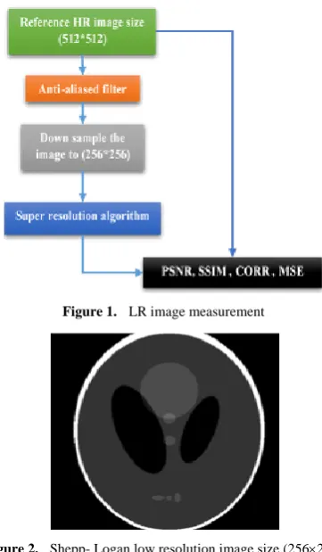
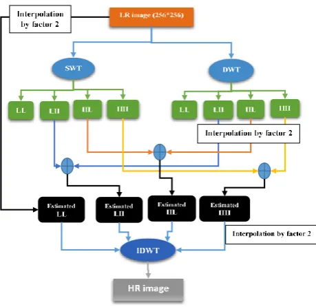
Super resolution of the image is the process of obtaining high resolution image from low resolution imageShepp-Logan image for the medical image, has taken, of size (256×256), which has down sampled from size (512×512) using Bicubic interpolation, where the anti-aliased filter has used before down sampling process to use it as the input image to the algorithm to enlarge it to the output of the size (512×512) pixels. The results show increasing the PSNR of the magnified image with respect to the original high resolution image. Where we has used the discrete wavelet transform, lifting wavelet transform with stationary wavelet transform, the traditional interpolation (Bicubic, Bilinear...etc.) and second order derivative directional interpolation (ICBI, DCC) has used to enlarge the sub bands, where the results has stated that the proposed schemes has different reconstruction images in both the edges and smooth area. Therefore, we take the less differences with the original reconstructed image and regard it as the super resolution image and denoising the images with FIR filter to reach and note the small effects on the images with the helping of the image quality metrics (PSNR, CORR, MSE, SSIM).Keywords
Wavelet transform, Super resolution, Interpolation, Edge directional interpolation, SWT, LWT, DWT, FIR filter, Directional cubic convolution (DCC) interpolation, ICBI (iterative curvature basic interpolation)1. Introduction
Wavelet transform is used by many researchers to achieve super resolution of the image [1-8]. The function of Wavelet transform is to disassemble signals of image and it has been used in image analysis. The original image contains LF component and aliased high frequency component so the decomposition level may obtain the fine resolution of high frequency component and edges texture. This is much important to obtain all HR component where the interpolation kernels have may be smoothing the HR signals. So the interpolation kernels (directional and average) has used in the wavelet transform to obtain the magnified image for each sub bands. And interpolation is achieved then fusing of the chosen sub bands that leading to large signal to noise ratio [9].
1.1. Medical Reconstructed Image
The test of the medical image used (Shepp-Logan) of size (512
×
512) filtered using anti-aliased filter, and then down sampled to (256×
256) in Bicubic interpolation to gives the* Corresponding author:
[email protected] (Muthana N. Abdul-Hussein Al-Hassany) Published online at http://journal.sapub.org/computer
Copyright©2018The Author(s).PublishedbyScientific&AcademicPublishing This work is licensed under the Creative Commons Attribution International License (CC BY). http://creativecommons.org/licenses/by/4.0/
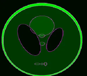
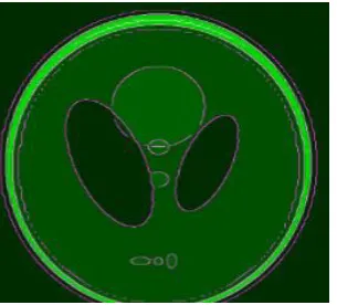
input low resolution image [17], see Figure 1 and Figure 2:
Figure 1. LR image measurement
1.2. Wavelet Transforms
The wavelets transform include discrete wavelet transform according to wavelet functions ψ(x) which it defined over a finite interval and having an average value of zero.
The basic idea of the wavelet is to represent any arbitrary function of time as a superposition of a set of such wavelets or basis functions.
These basis functions or baby wavelets are obtained from a single prototype wavelet called the mother wavelet, by dilations or contractions (scaling) and translations (shifts) [10, 11].
The wavelet are designed to give good time resolution and poor frequency resolution of high frequencies, and good frequency resolution and poor time resolution at low frequencies. This function is called scaling function (mother function) φ x , and under certain conditions which is the properties of the wavelet function the wavelet function can be generated as [12]:
ψ x = −1 k 𝑏
𝑘 φ 2x − k ∞
k=−∞
(1)
The DWT is generated by sampling the wavelet parameters 𝑎𝑘, 𝑏𝑘 on a grid or lattice. The reconstruction of the signal from its transform values naturally depends on the coarseness of the sampling grid [13].
A fine grid mesh would permit easy reconstruction, but with evident redundancy, i.e., oversampling. A too-coarse grid could result in loss of information [14].
The DWT of a signal x is calculated by passing it through a series of filters. First the samples are passed through a low pass filter with impulse response 𝑔 resulting in a convolution of the two, as in equation below:
y n = x ∗ g = +∞ x k g[n − k]
k=−∞ (2) The filter outputs down-sampled by 2 (multiplying each n by 2) which is decimation process in the filter bank and the following equations describe the decomposition process of x[k] according to filters g and h impulse response:
ylow n = +∞k=−∞x k . g[2n − k] (3)
𝑦ℎ𝑖𝑔ℎ 𝑛 = +∞𝑘=−∞𝑥 𝑘 . ℎ[2𝑛 − 𝑘] (4) DWT decomposes an image into different subband images; namely, average (LL), vertical (HL), horizontal (LH) and diagonal (HH) information and we have tested the SWT with it.
The lifting of the wavelet transform (LWT) is used to decompose the second generation wavelet, which basis function is called ‘lazy wavelet’. It has the formal property of wavelet, and which are not necessarily translates and dilates of one function. The latter we refer to as first generation wavelets, the lifting wavelet transform does not need auxiliary memory, but it just replaces the wavelet transform.
This lifting scheme is a new basis wavelet function added to build a new wavelet [15].
Lifting is a transform, which uses two operations in the decomposition; these are the update, and differences. As can be seen, the splitting of the even and odd samples is to predict the correlation between consecutive samples (even and odd) which result has no difference if it is equal. Similarly, the update gives the mean to the output sj-1 while the predict gives the gradient to the dj-1 output value [16]. See Figure 3:
Figure 3. LWT block diagram
2. Suggested Methods
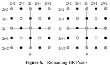
We describe the proposed methods, the LR image of size(256) has injected to the DWT and SWT filter bank the output (LH, HL, HH) subbands has added together but the (LL) subband which is the low frequency component has taken from the original LR image after interpolation of the entire bands with the traditional kernels then the invers discrete wavelet transform has achieved (IDWT) for the entire signals reconstruction the result of each interpolation kernels stated in the Table 3while the block diagram of the method is explained in the Figure 4:
The other simplest form which is the LWT, SWT where this method used the directional interpolation to accurate edges interpolation along the edges not across it and each subbands of LWT interpolated to much the size of the SWT sub bands and also the (LL) has taken from the original image after interpolation by factor 2.
Figure 5. LWT and SWT
In Figure 5, the SWT does not down sample the input LR image and the LWT does the down sampling of the input image that causes a loss of HF component. This is compensated by SWT by adding the HF component to the decomposition of LWT.
But the LWT in super resolution uses the directional interpolation to achieve fine results, therefore, we limit the result on how we use the interpolation in LWT and the reconstruction of it, also, we present the results of the DWT and DWT&SWT and the result of the FIR filter in the case of DWT&SWT in the tables illustrated, and we present the other results in the form of figures with different reconstruction options.
The directional interpolation which is used in our proposed scheme, include the ICBI (Iterative curvature based interpolation) and DCC (Directional Cubic Convolution) interpolation, where the interpolation formulas described below:
1-DCC: directional cubic convolution interpolation used the two gradient equations below to calculate the direction of edges:
For 45 diagonal computed in the 7
×
7 neighbourhoodG1=∑m=3,±1∑ n=3,±1|I(i+m,j-n)-I(i+m-2,j-n+2)| (5)
And For 135 diagonal
G2=∑m=3,±1∑ n=3,±1|I(i+m,j+n)-I(i+m-2,j+n-2)| (6)
Where the gradient direction computed for the neighbouring pixels:
Figure 6. Remaining HR Pixels
And the remaining steps window is as in the figure below:
G1=∑m=±1∑n=0,2|I(i+m,j-n)-I(i+m,j-n+2)|
+∑m=0,±2|I(i+m,j-1)-I(i+m,j+1)| (7)
G2=∑m=0,2∑n=±1|I(i-m,j+n)-I(i-m+2,j+n)|
+∑n=0,±2|I(i-1,j+n)-I(i+1,j+n)| (8)
If (1+G1)/(1+G2) > T The pixel on 135 or vertical strong edge else if (1+G1)/(1+G2)< T, the pixel (i, j) is on a 45° or horizontal strong edge; else the pixel (i, j) is in a weak or textured region; Where 1 is added to avoid gradients division by zero, assuming that the two orthogonal directional CC interpolation values at location(i, j) are I1(45°) diagonal or horizontal directional interpolation value)and I2(135°) diagonal or vertical directional interpolation value)the weights combining I1 and I2 are computed as
W1=1/1+G1k, W2=1/1+G2k (9)
Where k is an exponent parameter to adjust the weighting effect [1] and
I=(w1I1+w2I2)/( w1+w2) (10)
2- ICBI: where in this approach the gradient window are different in the edges as below:
Figure 7. Directional gradient diagonal
And the gradient is as below:
I ̃11(2i+1,2j+1)=I(2i-2,2j+2)+I(2i,2j)+I(2i+2,2j-2)-
3I(2i,2j+2)-3I(2i+2,2j)+I(2i,2j+4)+I(2i+2,2j+2)+
I(2i+4,2j) (11) I ̃22(2i+1,2j+1)=I(2i,2j-2)+I(2i+2,2j)+I(2i+4,2j+2)-
3I(2i,2j)-3I(2i+2,2j+2)+I(2i-2,2j)+I(2i,2j+2)+
So I11 and I22 are the estimated directional derivative in
the digonal direction and the other missing HR pixels are interpolated in the same way, which are lies in the horizontal and vertical direction of the LR neighbours. The pixel (2i+1, 2j+1) is computed as the average of the two neighbors in the direction where the derivative is lower.
And iterative manner is achieved on the interpolated pixels then the energy term defined for each interpolated pixel are minimized by small change in the second order derivative, where the energy term sums the local directional change of the second order derivatives.
3. FIR Filter
The FIR filter has been used in the image processing due to linear phase characteristics and any filters with non-linear phase can introduce artifacts that are visually annoying. The linear-phase FIR filter has been classified into four basic types as in Table 1 below:
Table 1. FIR filters types
Type Impulse response
I symmetric Length is odd
II symmetric Length is even
III Anti-symmetric Length is odd
IV Anti-symmetric Length is even
The chosen filter length N=35 is less than the all input samples and symmetric type I is convenience as a low pass filter. The use of the hamming window in time domain is to design FIR filter by convolving with 0.5 amplitude 𝑠𝑖𝑛𝑐 function to reduce the Gibbs ripples and reduce the side loop amplitude but the disadvantage is the increasing in the transition width.
4. Results and Discussion
The results are placed in two parts where the highly differences have been placed in the form of figures and the little differences have been placed in the form of tables of PSNR, Mean Square Error (MSE), Correlation, and Structure Similarity Measurement (SSIM). The results of using FIR filter with various nonlinear interpolation methods increased the quality of the medical image as seen in the Tables 2, 3, 4:
Table 2. Discrete Wavelet Transform
PSNR PSNR
(db) SSIM MSE CORR
Nearest 18.9862 29.4371 0.9015 0.0126 0.8686
Bilinear 23.6013 31.6130 0.9283 0.0044 0.9528
Bicubic 24.4631 31.9717 0.9307 0.0036 0.9601
Box 23.7044 31.6566 0.9377 0.0043 0.9525
Triangle 23.6013 31.6130 0.9283 0.0044 0.9528
Lanczos2 24.4532 31.9676 0.9309 0.0036 0.9600
Lanczos3 24.2487 31.8836 0.9147 0.0038 0.9584
Spline 24.2192 31.8714 0.9251 0.0038 0.9578
Makima 24.5016 31.9874 0.9331 0.0035 0.9606
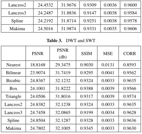
Table 3. DWT and SWT
PSNR PSNR
(db) SSIM MSE CORR
Nearest 18.8168 29.3475 0.9030 0.0131 0.8593
Bilinear 23.9074 31.7419 0.9295 0.0041 0.9562
Bicubic 24.8367 32.1232 0.9324 0.0033 0.9635
Box 24.1001 31.8222 0.9388 0.0039 0.9566
Triangle 24.0506 31.8016 0.9317 0.0039 0.9574
Lanczos2 24.8382 32.1238 0.9324 0.0033 0.9635
Lanczos3 24.7458 32.0865 0.9199 0.0034 0.9628
Spline 24.8504 32.1287 0.9328 0.0033 0.9636
Makima 24.7802 32.1005 0.9345 0.0033 0.9630
Table 4. FIR filter enhancement of DWT&SWT
PSNR PSNR(db) SSIM MSE CORR
Nearest 19.2541 29.5772 0.9014 0.0119 0.8709
Bilinear 23.9085 31.7423 0.9295 0.0041 0.9562
Bicubic 24.8451 32.1266 0.9323 0.0033 0.9635
Box 24.5438 32.0046 0.9420 0.0035 0.9609
Triangle 24.0516 31.8020 0.9317 0.0039 0.9575
Lanczos2 24.8471 32.1274 0.9323 0.0033 0.9636
Lanczos3 24.7576 32.0913 0.9201 0.0033 0.9629
Spline 24.8588 32.1321 0.9327 0.0033 0.9637
Makima 24.7883 32.1037 0.9344 0.0033 0.9631
We have seen in the Tables 2, 3, 4 the Makima interpolation outperforms others interpolations used in DWT in MSE and CORR, PSNR, but less than in SSIM value of Box interpolation. The spline interpolation has preferred in the case of DWT & SWT and FIR filter and the Box is more than in SSIM than other methods. Moreover, the lifting wavelet transform, in which the DCC [18] (Directional Cubic Convolution) interpolation and ICBI [19] (Iterative Curvature Based Interpolation) is used to achieve the finer result for the super resolution image. As seen in the Table 5:
Table 5. Lifting Wavelet Transform
LWT DCC
Haar
DCC db2
ICBI Haar
ICBI db2
PSNR 21.695 20.9399 21.6621 21.6875
PSNR (db) 30.7710 30.4166 30.7557 30.7674
MSE 0.00676 0.0081 0.0068 0.0068
SSIM 0.90387 0.8822 0.8988 0.8658
CORR 0.92489 0.9111 0.9240 0.9252
The results state that ‘Haar’ wavelet with DCC (Directional Cubic Convolution) outperforms the other methods in all measurement except the correlation between the two images. Where the ICBI with ‘db2’ wavelet gives the higher value in Correlation (0.9252). The nonlinear interpolation does not work with the lifting wavelet transform, as it gives bad image reconstruction in all measurements. Therefore, we have used the edge interpolation above to achieve the LWT super resolution with the result stated above.
The other results have illustrated in Figures 8, 9, in which lifting wavelet reconstruction with SWT has been used, where the difference with the original image illustrated has different colour and compared with Figure 10 which shows the DWT and SWT output image. Figure 11, 12 is the output image of the FIR filter and Figure 13 uses the Bicubic interpolation only.
Figure 8. LWT & SWT, DCC
Figure 9. LWT & SWT, ICBI
Figure 10. DWT & SWT
Figure 11. DWT & SWT FIR DCC
Figure 12. DWT & SWT, ICBI, FIR
Figure 13. Bicubic Only
We have tested the other reconstruction using SWT with DCC interpolation for each sub bands and FIR of the output image as seen in Figure 14:
The DWT with the DCC interpolation of each sub bands has used and the FIR filter has used to reach the desired value as we see in the Figure 15:
Figure 15. DWT DCC FIR
5. Conclusions
The conclusion which is appeared from the results in the figures above where the edges pixel have altered and if we use the FIR filter to reduce the noisy pixels, the wavelet transform scheme in Figure 11, 12 have less distortion in the reconstruction and can be taken to obtain the super resolution of the medical image which is better than other reconstructed images. Because it compsed from the directional interpolation of the edges (high frequency signals) and redundancy wavelet transform (SWT) which the results is benefit in this suggested methods.
Abbreviations
SWT (Stationary Wavelet Transform), LWT (Lifting Wavelet Transform), DWT (Discrete Wavelet Transform), HF (High Frequency), LF (Low Frequency). PSNR (Peak Signal to Noise Ratio). CWT (Continuous Wavelet Transform). LR (Low Resolution), HR (High Resolution),
SSIM (Structure Similarity Measurement), CORR
(Correlation).
REFRENCES
[1] S.-C. Tai, T.-M. Kuo, C.-H. Iao, and T.-W. Liao, “A Fast Algorithm for Single Image Super Resolution in Both Wavelet and Spatial Domain,” 2012 Int. Symp. Comput. Consum. Control, pp. 702–705, 2012.
[2] C. V. Jiji, M. V. Joshi, and S. Chaudhuri, “Single-frame image super-resolution using learned wavelet coefficients,” Int. J. Imaging Syst. Technol., vol. 14, no. 3, pp. 105–112, 2004.
[3] H. Demirel and G. Anbarjafari, “Image resolution enhancement by using discrete and stationary wavelet decomposition.” IEEE Trans. Image Process, vol. 20, no. 5, pp. 1458–1460, 2011.
[4] M. D. Robinson, C. A. Toth, J. Y. Lo, and S. Farsiu, “Efficient fourier-wavelet super-resolution,” IEEE Trans. Image Process., vol. 19, no. 10, pp. 2669–2681, 2010. [5] L. Shen and Q. Sun, “Biorthogonal wavelet system for
high-resolution image reconstruction,” IEEE Trans. Signal Process, vol. 52, no. 7, pp. 1997–2011, 2004.
[6] G. Anbarjafari and H. Demirel, “Image super resolution based on interpolation of wavelet domain high frequency subbands and the spatial domain input image,” ETRI J., vol. 32, no. 3, pp. 390–394, 2010.
[7] M. Agrawal and R. Dash, “Image resolution enhancement using lifting wavelet and stationary wavelet transform,” Proc. - Int. Conf. Electron. Syst. Signal Process. Comput. Technol. ICESC 2014, pp. 322–325, 2014.
[8] F. Zhou, W. Yang, and Q. Liao, “Interpolation-based image super-resolution using multisurface fitting,” IEEE Trans. Image Process., vol. 21, no. 7, pp. 3312–3318, 2012. [9] S. Fadnavis, “Image Interpolation Techniques in Digital
Image Processing: An Overview,” Int. J. Eng. Res. Appl., vol. 4, no. 10, pp. 70–73, 2014.
[10] G. P. Nason and B. W. Silverman, “The stationary wavelet transform and some statistical applications,” Wavelets Stat., pp. 281–299, 1995.
[11] D. Bharath Bhushan, V. Sowmya, and K. P. Soman, “Super resolution blind reconstruction of low resolution images using framelets based fusion,” ITC 2010 - 2010 Int. Conf. Recent Trends Information, Telecommun. Comput., no. May 2016, pp. 100–104, 2010.
[12] T. Li, Q. Li, S. Zhu, and M. Ogihara, “A survey on wavelet applications in data mining,” ACM SIGKDD Explore. Newsl. vol. 4, no. 2, pp. 49–68, 2002.
[13] T. Acharya and P.-S. Tsai, “Computational Foundations of Image Interpolation Algorithms,” Ubiquity, vol. 8, no. 42, p. 4:1–4:17.
[14] A. N. Akansu and R. A. Haddad, Multiresolution Signal Decomposition: Transforms, Subbands, and Wavelets, Second edition, new jersey: Academic Press, 2001.
[15] W. Sweldens, “Wavelets and the lifting scheme: A 5 minute tour,” Z. Angew. Math. Mech., vol. 76, no. Suppl. S2, pp. 41–44, 1996.
[16] S. Naik and V. Borisagar, “A Novel Super Resolution Algorithm Using Interpolation and LWT Based Denoising Method,” Int. J. Image Process., vol. 6, no. 6, pp. 198–206, 2012.
[17] N. H. F. Al-anbari and M. H. A. Al-hayani, “Design and Construction Three-Dimensional Head Phantom Test Image for the Algorithms of 3D Image Reconstruction,” vol. 6, no. 2, pp. 98–104, 2015.
[18] D. Zhou, W. Dong, and X. Shen, “Image zooming using directional cubic convolution interpolation,” IET Image Process., vol. 6, no. 6, pp. 627–634, 2012.