Novel method for identifying wheat leaf disease images based on
differential amplification convolutional neural network
Mengping Dong
1,
Shaomin Mu
1*,
Aiju Shi
2,
Wenqian Mu
1,
Wenjie Sun
1(1. College of Information Science and Engineering, Shandong Agricultural University, Taian, Shandong 271018, China; 2. College of Chemistry and Materials Science, Shandong Agricultural University, Taian, Shandong 271018, China)
Abstract: In this study, a differential amplification convolutional neural network (DACNN) was proposed and used in the identification of wheat leaf disease images with ideal accuracy. The branches added between the deep convolutional layers can amplify small differences between the real output and the expected output, which made the weight updating more sensitive to the light errors return in the backpropagation pass and significantly improved the fitting capability. Firstly, since there is no large-scale wheat leaf disease images dataset at present, the wheat leaf disease dataset was constructed which included eight kinds of wheat leaf images, and five kinds of data augmentation methods were used to expand the dataset. Secondly, DACNN combined four classifiers: Softmax, support vector machine (SVM), K-nearest neighbor (KNN) and Random Forest to evaluate the wheat leaf disease dataset. Finally, the DACNN was compared with the models: LeNet-5, AlexNet, ZFNet and Inception V3. The extensive results demonstrate that DACNN is better than other models. The average recognition accuracy obtained on the wheat leaf disease dataset is 95.18%.
Keywords: convolutional neural network, differential amplification, wheat leaf diseases, image identification DOI: 10.25165/j.ijabe.20201304.4826
Citation: Dong M P, Mu S M, Shi A J, Mu W Q, Sun W J. Novel method for identifying wheat leaf disease images based on differential amplification convolutional neural network. Int J Agric & Biol Eng, 2020; 13(4): 205–210.
1 Introduction
Wheat is one of the most important rations in China. The development of the wheat industry is related to the country's food security and social stability directly. Therefore, it is important for yield and quantity to recognize wheat leaf diseases. However, at present, the main method of wheat leaf disease identification is manual identification, which has low efficiency and accuracy.
In recent years, deep learning has developed in image recognition. In 1998, LeNet-5 was used for postal code handwriting recognition, which has a 7-layer network structure[1].
In 2012, Convolutional Neural Network (CNN) was used to achieve the best result in the ImageNet large-scale visual recognition challenge, which caused to receive widespread attention[2]. In 2014, Zeiler et al.[3] implemented ZFNet to
visualize network structure through deconvolution technology. Simonyan et al.[4] proposed the visual geometry group (VGG)
model that increased the depth of the network by adding a convolution layer of 3×3 convolution kernels, and used a small convolution kernel to replace a convolution layer with a larger convolution kernel, reducing the number of parameters. In 2015,
Received date: 2018-12-04 Accepted date: 2020-05-27
Biographies: Mengping Dong, Graduate student, research interests: artificial intelligence, Email: [email protected]; Aiju Shi, Graduate student, researcher, research interests: pest control, Email: [email protected]; Wenqian Mu, Undergraduate student, research interests: machine learning, Email: [email protected]; Wenjie Sun, Graduate student, research interests: artificial intelligence, Email: [email protected].
*Corresponding author: Shaomin Mu, PhD, Professor, research interests: machine learning, artificial intelligence, big data. College of Information Science and Engineering, Shandong Agricultural University, No.61 Daizong Street, Taian, Shandong 271018, China. Tel: +86-15005486826, Email: [email protected].
Szegedy et al.[5] proposed the GoogleNet with more than 20 layers,
which increased the depth of CNN, improved the utilization rate of the computer, reduced the parameters, and improved the accuracy. In 2016, through a series of correction methods that can increase accuracy and reduce computational complexity, Inception V2 and Inception V3 were proposed in the paper[6]. He et al.[7] used a residual network to solve the problem of vanishing gradients, so that the underlying network can be fully trained. As the depth increases, so does accuracy. The idea of cross-channel connection was further extended to multi-layer connections by DenseNet to improve representation[8]. In 2018, Khan[9] introduced a new channel improvement idea. The motivation for network training with channel boosted representations is to use rich representations. This idea effectively improved the performance of CNN by learning various features. In 2019, Hou et al.[10] proposed a method for selecting channels based on the relative of activation, and proposed weighted channel discarding for regularization of convolutional layers in CNN.
LeNet model to identify the diseases of cucumber, which was more accurate than traditional methods. Huang et al.[17] proposed that GoogleNet was used to identify disease images of spikes, and the classification effect was obvious. In 2017, the capsule network was proposed by Sabour et al.[18]. Since CNN cannot learn spatial relationships, the pooling layer will lose the information, and the capsule will adjust the output according to the changes. Deng et al.[19] proposed the capsule network to classify hyperspectral images, and the classification accuracy rate exceeded CNN. In 2018, Gan et al.[20] established a hyperspectral inversion model for
chlorophyll content prediction of longan leaves using sparse self-encoding of classic models of deep learning. The accuracy can be greatly improved by using deep learning methods. Zhu et al.[21] used the improved faster region-based convolutional network
(Faster-RCNN) to identify plant leaves, and achieved a high recognition accuracy than Faster RCNN in the complex background.
With the increase of network depth, large network models tend to ignore light feedback errors, which lead to lower convergence rates[7]. Finally, the large deepening model itself tends to ignore the details of large-scale data. In view of the above problem, this study proposes the differential amplification convolutional neural
network (DACNN), which can amplify small differences between the real output and the expected output. And it has achieved good results in the identification of wheat leaf disease images. The differential amplifier branches constructed in the deep neural layers can make the model more sensitive to the light error of each iteration feedback. It can alleviate the error omission. Since there is no large-scale wheat leaf disease images dataset at present, and the wheat leaf disease dataset was constructed.
2 Materials and methods
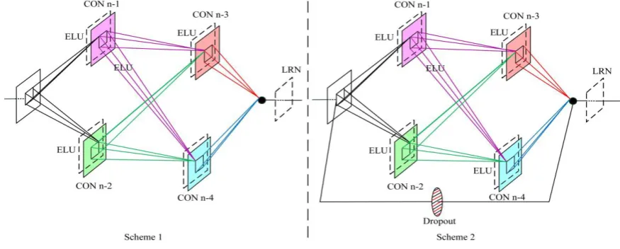
The DACNN contains 6 convolutional layers, 3 max-pooling layers and 3 fully connected layers. To improve the ability of feature extraction, 3×3 kernels are used to replace the larger kernels and convolution kernels are fully connected in the last two layers. In order to alleviate the omission of minor errors in the backpropagation pass, a branch is added before and after the deep convolution layer of the differential amplifier, so as to simulate the difference which achieves the function of error amplification. In Figure 1, the structure of the traditional CNN is compared with that of the differential amplification branch, and the advantage of the latter in the error amplification effect is proved by theoretical analysis.
Figure 1 Structure of differential amplification branch 2.1 Differential amplification branch
Scheme 1 in Figure 1 is the schematic diagram demonstrating the CNN that does not add a branch in deep neural layers, similar to the traditional CNN, whose data stream can be represented by Equation (1).
1 ( )
l i i l l
T E
w x b (1)where, w1 and b1 are the weight matrix and the bias of the lth neural
layer, respectively; xl is the mapping input and Tl+1 is mapping
result of the lth neural layer, respectively, and E() is a linear activation function.
Scheme 2 in Figure 1 is the schematic diagram demonstrating the CNN that adds a differential amplification branch in DACNN. Its data stream satisfies Equation (2).
1 ( , , )
( , , ) ( ), 0,1, 2,...,
l l l l l l
l l l l i i l l
H x F x w b
F x w b E w x b l L
(2)where, wland bl are the weight matrix and the bias of the lth neural layer, respectively; xl and Hl+1 are the mapping input and mapping
results of the lth neural layer, respectively; Fl () is the mapping output of convolutional layers and E() is the linear activation function. Compared to Scheme 1, this structure can strip the unchanged partxl and highlight the minor change of Fl (xl, wl, bl),
thus making the model more sensitive to error of the back- propagation pass during each iteration.
Suppose the input feature map is 100. It is expected mapping results and the actual mapping results in the convolutional layer are 105 and 110 respectively, and Δf6=5, as is shown in Equation (3).
6 5
6 5
5
( ) 105
( ) 110
100
f x f x x
(3)
f6 and f6′ represent the expected mappings and actual mappings of
the convolutional layer, respectively. ‘′’ represents functions and variables, etc. in actual situations. In Scheme 1, the ΔT6 is 5
which is shown in Equation (4).
6 5 5
6 5 5
( ) 105
( ) 110
i i
i i
T E w x b T E w x b
(4)The proportion of ΔT6 is shown in Equation (5).
6
6
6 5
0.0476 105
T
T P
T
(5)
In Scheme 2, there is
6 5 5 5 5 5
6 5 5 5 5 5
( , , ) 105
( , , ) 110
H x F x w b H x F x w b
Naturally,
5 5 5 5 5 5
5 5 5 5 5 5
( , , ) ( ) 5
( , , ) ( ) 10
i i
i i
F x w b E w x b F x w b E w x b
(7)And Δf5=5 are got. The proportion of Δf5 is shown in
Equation (8). 5 5 5 5 1 5 F F P F
(8)
Obviously, PF5 in Scheme 2 is much larger than PT6 in
Scheme 1. Therefore, the network structure in Scheme 2 can enlarge the error in backpropagation pass between the expected output and the actual output, which is beneficial to the correct convergence of the model.
Then, in Scheme 2, Equation (10) can be obtained by recursive Equation (9).
2 1 1 1 1
1 1 1
( )
( ) ( )
l l i i l l
l i i l l i i l l
x x E w x b
x E w x b E w x b
(9)1
( )
L
L l i l i i i i
x x
E
w x b (10)For the initial input x0 the mapping result of the Lth neural
layer satisfies Equation (11). 1
0 0 ( )
L
L i i i i i
x x
E
w x b (11)From Equations (10) and (11), it can be seen that the differential amplification effect can be accumulated layer by layer, thus improving the fitting ability of the model to image pixel distribution and the identification accuracy to a maximum extent. 2.2 Normalized layers
As noted above, owing to the influence of sunlight, water mist, dust, and other factors, the range of the signal intensity in gathered images is extremely wide. Signals with wide ranges of values often play a major role in model learning, and smaller range signals have less effect, thus affecting the trend of model coverage. Moreover, the range of the function domain is limited, so the input data need to be mapped into this domain. To solve the above problems, the local response normalization (LRN) is used before and after the differential amplification branch.
By creating a competition mechanism, LRN can make the activity of local neurons with the larger response, inhibit other neurons with smaller feedback, which improves the generalization ability of the model, and prevent the data from overfitting[2], as is shown in Equation (12).
min( 1, / 2)
( ) ( ) ( j) 2
, , / ( j= max(0, / 2)( , ) )
N i n
i i
p q p q i n p q
y x k
x (12)where, ( ) , i p q
y is the normalized value, and i is the position of the
channel, which represents the value of the update channel, and p
and q represent the position of the pixel. And the ( ) , i p q
x is the input value, α=0.0001 is the scaling factor, β=0.75 is the exponential term, n=5 is the local size of the normalized range. 2.3 Dropout
In order to improve the generalization ability and inhibit overfitting, the dropout strategy[22] is introduced in the differential amplification branch. When the network propagates forward, it stops a neuron with a certain probability of p, its activation function value change from probability p to 0. Dropout reduces the dependence between neurons by forcing a neuron to interact with randomly selected neurons and prevents some features from having effect only under other specific features. So that dropout can improve the generalization ability of the model. The dropout rate is set to 0.5 in this study, that is to say, when the neurons pass
dropout, half of them will be set to 0. Figure 2 illustrates the training process of DACNN with dropout.
Figure 2 Learning processing of DACNN with dropout In Equation (13), Bernoulli function is used to generate probability B vector, that is, randomly generate a vector of 0 and 1. And ( )l
i
y is the input of the upper layer. As is shown in Equation (14), ( )l
i
y is multiplied by the ( )l i
B to obtain the processed signal after masking ( )l
i
y . The output (l1) i
y is then calculated by the Equations (15) and (16). The whole procedure is indicated below.
( )
( ) l
i
B Bernoulli distribution p (13) ( )l ( )l ( )l
i i i
y B y (14)
(l 1) (l1) ( )l (l1)
i i i i
y w y b (15)
( 1) ( 1)
( )
l l
i i
y f y (16)
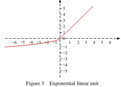
2.4 Exponential linear unit
In this paper, we use the exponential linear unit (ELU) as the nonlinear activation function, as shown in Equation (17).
0
( x 1) 0
x if x y
e if x
(17)
ELU is an improved version of the Rectified Linear Unit (ReLU). Compared to the ReLU function, when the input is negative, it has a certain output. As shown in Figure 3, the linear part of the right segment can alleviate the gradient disappearance, while the soft saturation end makes it more robust to input changes and noise at the left. The mean value of the output is close to 0, and the convergence speed of the ELU is fast.
Figure 3 Exponential linear unit 2.5 Experimental setup
core of TensorFlow.
Table 1 Basic Characteristics of GPUs
Configuration parameter Parameter value
Chip model NVIDIA GeForce GTX 1080
RAM capacity 8192M
RAM interface 256-bit
Core frequency 1759/1936 MHz
Memory frequency 10206/10400 MHz
Stream processor 2560
Raster processing unit 64
RAMDAC frequency 400 MHz
Maximum resolution 7680×4320
3 Construction of the dataset
As there are no large-scale images of wheat leaf diseases,
therefore, images were collected from several wheat planting bases in Shandong province. Then, they were expanded by 5 kinds of data augmentation techniques to construct the wheat leaf disease dataset. It is expected that these experiments can shorten the distance between the theoretical research of neural networks and the practical agricultural application.
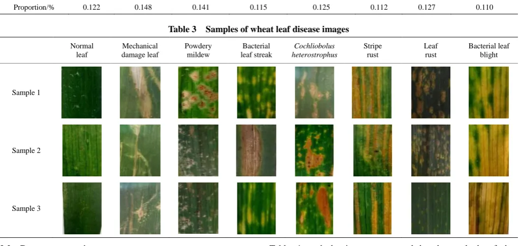
3.1 Acquisition of images
The wheat leaf images were collected from the wheat planting bases of Shandong Province of China. The number of the original dataset is 8326, containing normal leaf and 7 kinds of diseases, which are mechanical damage leaf, powdery mildew, bacterial leaf streak, cochliobolus heterostrophus, stripe rust, leaf rust and bacterial leaf blight. The images were taken with a Canon EOS 80D (18-200 mm). The image format is JPEG and each image is a 24-bit color bitmap. The numbers and proportions of the wheat leaf disease image in the original dataset are shown in Table 2, and the samples of wheat leaf disease images are shown in Table 3. Table 2 Number and proportion of the wheat disease image in original dataset
Name Normal leaf Mechanical damage leaf
Powdery mildew
Bacterial leaf streak
Cochliobolus
heterostrophus Stripe rust Leaf rust
Bacterial leaf blight
Number 1016 1237 1182 962 1046 939 1061 883
Proportion/% 0.122 0.148 0.141 0.115 0.125 0.112 0.127 0.110
Table 3 Samples of wheat leaf disease images
Normal leaf
Mechanical damage leaf
Powdery mildew
Bacterial leaf streak
Cochliobolus heterostrophus
Stripe rust
Leaf rust
Bacterial leaf blight
Sample 1
Sample 2
Sample 3
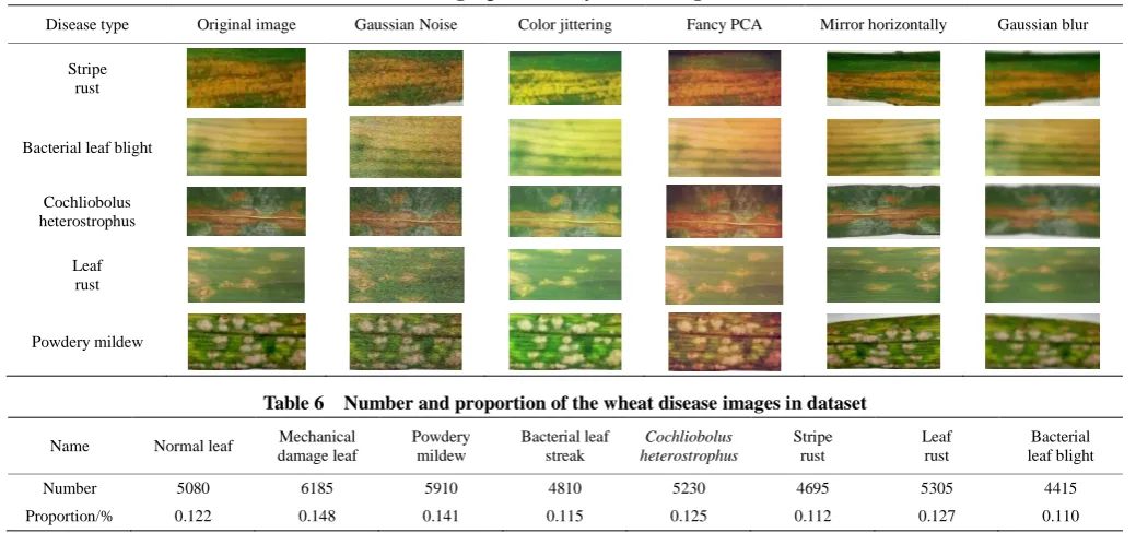
3.2 Data preprocessing
The CNN self-learning relies on iterative training on a large-scale dataset. If the amount of data is too small, it is prone to cause the overfitting, which makes the training error very small while the testing error very large[23]. In order to increase the size and diversity of original dataset, 5 ways are adopted to implement dataset augmentation which are add Gaussian noise, color jittering, fancy PCA, mirror horizontally and Gaussian blur, as shown in
Table 4, and the images processed by the methods of data augmentation are shown in Table 5.
Data augmentation can produce 6 corresponding enhanced images of every category of wheat leaf disease images. Finally, the number of data augmentation of wheat leaf diseases is 41630, the number and proportion of each kind of wheat leaf disease images are shown in Table 6.
Table 4 Method of data augmentation
Name Detail operations
Gaussian noise Add 30% Gaussian noise to the original image.
Color jittering Increase saturation and brightness by 20% and contrast by 30%. Fancy PCA
Change the intensity of RGB channel, then perform PCA on all RGB pixel values, and obtain a 3×3 covariance matrix; A new covariance moment is obtained by multiplying the eigenvalue by a random variable with a mean value of 0 and a standard deviation of 0.1 Gaussian distribution.
Mirror horizontally Mirror the left and right parts of the image with the vertical central axis of the image as the center.
Table 5 Images processed by the data augmentation
Disease type Original image Gaussian Noise Color jittering Fancy PCA Mirror horizontally Gaussian blur Stripe
rust
Bacterial leaf blight Cochliobolus heterostrophus
Leaf rust
Powdery mildew
Table 6 Number and proportion of the wheat disease images in dataset
Name Normal leaf Mechanical damage leaf
Powdery mildew
Bacterial leaf streak
Cochliobolus heterostrophus
Stripe rust
Leaf rust
Bacterial leaf blight
Number 5080 6185 5910 4810 5230 4695 5305 4415
Proportion/% 0.122 0.148 0.141 0.115 0.125 0.112 0.127 0.110
4 Results and discussion
4.1 DACNN-Softmax, DACNN-SVM, DACNN-KNN and DACNN-Random Forest
In this experiment, DACNN is combined with softmax, support vector machine (SVM), K-nearest neighbor (KNN), and Random Forest to identify the augmented dataset, which aims at investigating the effect of different classifiers on identification results by observing their trend of accuracy change. In KNN, k is set to 100. Radius Basis Function (RBF) is used in SVM. The penalty parameter C, γ, and slack variable ζ are initialized to 10, 0.02 and 0.001, respectively. The number of decision trees in Random Forest is 200, and the Gini index is used:
2
( ) 1 ci i
Gini D
p , where c represents the number of categories in the dataset and is set to 8. pi represents the proportion of the ith category of samples in all samples. The 4 models are iterated 50000 times on the augmented dataset, and save the intermediate model every 5000 iterations and validation it with the test dataset. Their change procedure of identification accuracy is shown in Figure 4.Figure 4 Accuracy of DACNN-Softmax, DACNN-SVM, DACNN-KNN and DACNN-Random Forest
It can be seen from Figure 4 that when the models are convergent, the identification accuracy of DACNN-SVM and
DACNN-Softmax are 95.32% and 96.09%, respectively, which is obviously superior to the accuracies of DACNN-KNN and DACNN-Random Forest of 90.37% and 89.96%. Furthermore, through the experiment process, we can see that the identification
accuracy of DACNN-SVM is higher than that of
DACNN-Softmax when the number of iterations is small. This is because the number of iterations is small and the data throughput is small in the early experiment, and SVM is just a classification algorithm based on statistical learning theory, which replaces Empirical Risk Minimization (ERM) with Structure Risk Minimization (SRM). It is suitable for small sample data classification, so it has higher recognition accuracy than Softmax in the early stage.
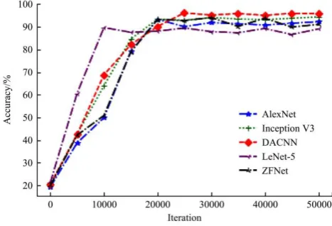
4.2 DACNN, Inception V3, LeNet-5, AlexNet and ZFNet In order to verify the performance of DACNN, it is compared with Inception V3, Lenet-5, AlexNet and ZFNet. LeNet-5 consists of 3 convolutional layers, 2 subsampling layers, and 3 fully connected layers, which have been widely used in digital handwriting recognition; Both AlexNet and ZFNet contain 5 convolutional layers, 3 subsampling layers, and 3 fully connected layers. However, the former uses two GPU sparse connection structures, while ZFNet uses only one GPU dense connection structure. Inception V3 works by performing multiple convolution and pooling operation on the image and outputs a deep feature map. In the above experimental environment, the 5 models are iterated 50 000 times on the augmented dataset and save the intermediate model every 5 000 iterations and validation it with the test dataset. The training process of the model is shown in Figure 5.
Figure 5 Training process of DACNN, Inception V3, Lenet-5, AlexNet and ZFNet
5 Conclusions
In this study, we deal with the recognition of the wheat leaf disease image by proposing a novel method named DACNN, a differential amplification convolutional neural network. Especially, branches before and after the deep convolution layer in DACNN were added to simulate the differential amplifier and realize the function of error amplification. Then, there is no standard dataset of wheat leaf diseases, constructing the wheat leaf disease dataset. Finally, the experimental results with Inception-V3, AlexNet, ZFNet and LeNet-5 and combined with four classifiers, which are Softmax, SVM, KNN and Random Forest on the wheat leaf diseases dataset show the superiority of DACNN. For future work, we plan to apply DACNN to other types of visual tasks, such as object detection.
Acknowledgements
This work is supported by First Class Discipline Funding of Shandong Agricultural University (XXXY201703).
[References]
[1] Lecun Y, Bottou L, Bengio Y, Haffner P. Gradient-based learning applied to document recognition. Proc.IEEE, 1998; 86(11): 2278–2324. [2] Krizhevsky A, Sutskever I, Hinton G E. ImageNet classification with
deep convolutional neural networks. Proceedings of Advances in Neural Information Processing Systems, 2012; 25: 1097−1105.
[3] Zeiler M D, Fergus R. Visualizing and understanding convolutional networks. Computer Vision-ECCV, IEEE, 2014; 8689: 818–833. [4] Simonyan K, Zisserman A. Very deep convolutional networks for
large-scale image recognition. arXiv preprint, 2014; 6: 1–47. arXiv 1409.1556.
[5] Szegedy C, Liu W, Jia Y, Sermanet P, Reed S, Anguelov D, et al. Going deeper with convolutions. In: 2015 IEEE Conference on Computer Vision and Pattern Recognition (CVPR), Boston: IEEE, 2015; pp.1–9. [6] Szegedy C, Vanhoucke V, Ioffe S, Shlens J, Wojna Z. Rethinking the
inception architecture for computer vision. IEEE Conference on Computer Vision and Pattern Recognition, IEEE, 2016; pp.2818–2826. [7] He K M, Zhang X Y, Ren S Q, Sun J. Deep residual learning for image
recognition. In: 2016 IEEE Conference on Computer Vision and Pattern Recognition (CVPR), Las Vegas: IEEE, 2016; pp.770–778.
[8] Huang G, Liu Z, Laurens V D M, Weinberger K Q. Densely connected convolutional networks. Computer Vision and Pattern Recognition, IEEE, 2017; pp.4700-4708. doi: 10.1109/CVPR.2017.243.
[9] Khan A, Sohail A, Ali A. A new channel boosted convolutional neural network using transfer learning. arXiv preprint, 2018. arXiv:1804.08528. [10] Hou S H, Wang Z L. Weighted channel dropout for regularization of
deep convolutional neural network. AAAI Conference on Artificial Intelligence, 2019; 33: 8425–8432.
[11] Zeng W H, Li M, Li Z, Xiong Y. High-order residual and parameter-sharing feedback convolutional neural network for crop disease recognition. Acta Electronica Sinica, 2019; 47(9): 1979–1986.
[12] Zhang K, Guo Y R, Wang X S, Yuan J S, Ding Q L. Multiple feature reweight Dense Net for image classification. IEEE Access, 2019; 7: 9872–9880.
[13] Amanda R, Kelsee B, Peter M, Babuali A, James L, David P. Deep learning for image-based cassava disease detection. Frontiers in Plant Science, 2017; 8: 1852. doi: 10.3389/fpls.2017.01852.
[14] Mohanty S P, Hughes D P, Salathé M. Using deep learning for image-based plant disease detection. Frontiers in Plant Science, 2016; 7: 1419. doi: 10.3389/fpls.2016.01419.
[15] Lu Y, Yi S J, Zeng N Y, Liu Y R, Zhang Y. Identification of rice diseases using deep convolutional neural networks. Neurocomputing, 2017; 267(Dec.6): 378–384.
[16] Zhang S W, Xie Z Q, Zhang Q Q. Application research on convolutional neural network for cucumber leaf disease recognition. Jiangsu Journal of Agricultural Sciences, 2018; 34(1): 56 – 61.
[17] Huang S P, Sun C, Qi L, Ma X, Wang W J. Rice panicle blast identification method based on deep convolution neural network. Transactions of the CSAE, 2017; 33(20): 169 – 176.
[18] Sabour S, Frosst N, Hinton G E. Dynamic routing between capsules. Neural Information Processing Systems, 2017; pp.3856–3866.
[19] Deng F, Pu S L, Chen X H, Shi Y S, Yuan T, Pu S Y. Hyperspectral image classification with capsule network using limited training samples. Sensors, 2018; 18(9): 3153. doi: 10.3390/s18093153.
[20] Gan H M, Yue X J, Hong T S, Ling K J, Wang L H, Cen Z Z. A hyperspectral inversion model for predicting chlorophyll content of Longan leaves based on deep learning. Journal of South China Agricultural University, 2018; 39(3): 102–110. (in Chinese)
[21] Zhu, X L, Zhu M, Ren H. Method of plant leaf recognition based on improved deep convolutional neural network. Cognitive Systems Research, 2018; 52(Dec.): 223–233.
[22] Srivastava N, Hinton G, Krizhevsky A Sutskever I, Salakhutdinov R. Dropout: A simple way to prevent neural networks from overfitting. Journal of Machine Learning Research, 2014;15: 1929–1958.