Robust Performance Analysis for a Cascade Nonlinear H∞ Control Algorithm In Quadrotor Position Tracking

(1)

AUT Journal of Mechanical Engineering

AUT J. Mech. Eng., 4(2) (2020) 151-168 DOI: 10.22060/ajme.2019.15561.5779

Robust Performance Analysis for a Cascade Nonlinear H∞ Control Algorithm in

Quadrotor Position Tracking

F. Rekabi, F. A. Shirazi*, M. J. Sadigh

School of Mechanical Engineering, College of Engineering, University of Tehran, Tehran, Iran

ABSTRACT: This paper presents a new hierarchical robust algorithm to solve the position tracking problem, in presence of exogenous disturbances and modeling uncertainties, of a quadrotor helicopter. The suggested controller includes a nonlinear H∞ algorithm to track the reference trajectory in the outer

loop and a nonlinear H∞ controller to stabilize the rotational movements in the inner loop. The resultant

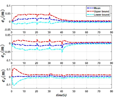
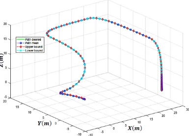
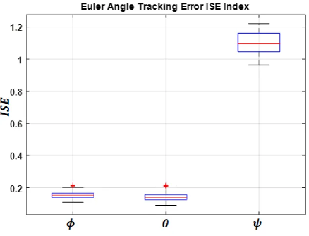
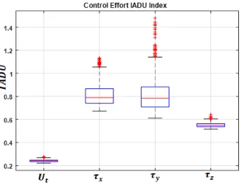
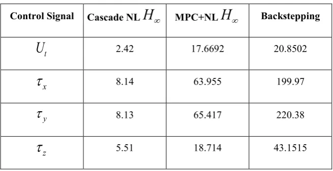
controller consists of three important parts to regulate tracking errors for translational and rotational motions, maintain robust performance confronting random disturbances and modeling uncertainties and reject the sustained disturbances from the system to vanish the steady-state errors. Analytical study on the stability of the cascade system is mentioned to verify the compatibility of two controllers considering coupling terms. Numerical performance analysis is accomplished using Monte-Carlo simulation. Statistical results obtained from 1000 simulations considering environmental disturbances and modeling uncertainties depict less than 5 cm for position tracking error and less than 2 degrees for attitude tracking error in steady state performance. The closed-loop performance of the controller is also compared with two previous algorithms by determining two numerical indexes for state tracking performance and control efforts, respectively. Simulation results of the suggested control algorithm depict a significant reduction in both indexes for a similar mission.

Review History: Received: 31 Dec. 2018

Revised: َ7 Apr. 2019 Accepted: 5 May. 2019 Available Online: 11 May. 2019

Keywords: Position tracking Nonlinear H∞ control

Cascade control Stability analysis

151 1- Introduction

Unmanned aerial vehicles, especially multirotors, have attracted a great interest in the automatic control area in last few decades due to their special advantages such as simple structure, vertical take-off and landing, rapid maneuvering and precise hovering. These vehicles have been used in tasks such as search and rescue, building exploration and security, and industrial inspections [1-3]. Although these vehicles have a high capability in aerial missions, their stabilization and control is challenging. The unstable and under-actuated nature of these systems makes the controller design procedure more complicated. Furthermore, quadrotors usually operate in presence of environmental disturbances such as wind gusts. Thus, quadrotors require not only a fast response hardware system but also a high performance control algorithm capable of confronting exogenous disturbing effects and uncertainties [4,5].

Control system design for quadrotors, has been highlighted in a number of papers and researchers have tried to satisfy the specifications by utilizing various techniques. In practice, especially in civil applications, low-cost equipment has been used for hardware, therefore it is crucial to compensate the consequent weaknesses by designing a simple structure algorithm with low computational burden for practical implementation. This controller has to consider the nonlinearities of the system and guarantees

the stability of the closed-loop system [6-8]. Another work which presented a simple control algorithm to stabilize the quadrotor platform was presented in reference [9]. It resulted in a simple controller suitable for an embedded use when low computational resources are available. Some researchers have proposed a set of more complicated sensors to increase the reliability of the localization and obstacle avoidance systems. For instance, in reference [10] a Disturbance Observer Based (DOB) design was proposed that estimated the disturbance based on a dynamic model and a sensor suite including ultrasonic range finder and InfraRed (IR) sensors. In this work, the experimental results for robust controller based on this observer represented a good performance in harsh environments dangerous for the human to work. To handle the model uncertainty and external disturbances, different techniques have been used by researchers such as radial basis function neural networks adopted in the attitude control design and the backstepping technique [11-13]. A method for robustness against both environmental disturbance and parametric uncertainty was presented by Nicol et al. [14] using Cerebellar Model Articulation Controller (CMAC) nonlinear approximators for an experimental prototype quadrotor helicopter. The method updates adaptive parameters, the CMAC weights, as to achieve both adaptation and robustness to unknown payloads and disturbances. In a similar work, a robust-optimal control was proposed to compensate the parameter uncertainty effects and disturbances in reference [15]. In another work a robust-optimal framework was suggested using neural network to solve the position tracking

*Corresponding author’s email: [email protected]

(2)

F. Rekabi et al., AUT J. Mech. Eng., 4(2) (2020) 151-168, DOI: 10.22060/ajme.2019.15561.5779

152 problem for a quadrotor helicopter [16].

In a different way, some researchers used linear and nonlinear adaptive approaches to solve the attitude stabilization and path following problem for aerial robots [17-20]. Moreover, researchers have tried to apply nonlinear methods to conftont the complex dynamic behavior of these systems and improve the flying performance [21-23]. An underactuated NonLinear H∞ (NLH∞) controller based on the six degrees of freedom dynamic model was designed by Raffo et al. [24] to control the helicopter attitude and altitude in the inner-loop. The outer-loop control was performed using a Model-based Predictive Controller (MPC) to track the reference trajectory. The robust performance achieved by the proposed control strategy was checked by simulations in presence of aerodynamic disturbances, unmodelled dynamics, and parametric uncertainties but no theoretical proof of stability was presented for the cascade structure. Another work presented a method based on the block control technique combined with the super twisting control algorithm for trajectory tracking of a quadrotor helicopter in 2011. The performance and effectiveness of the proposed controller were tested in a simulation study taking into account external disturbances [25]. In another approach, a linear time-invariant controller consisting of a Proportional-Derivative (PD) controller and a robust compensator was used for robust attitude control of uncertain quadrotors. The PD controller was designed for the nominal linear system to achieve the desired tracking and the robust compensator was added to limit the influence of uncertainties. The simplicity of the final structure of control scheme made it applicable for practical cases with a simple hardware [11, 26-27]. Liu et al. [26] proposed a robust hierarchical controller including an attitude controller and a position controller. The position controller generated the desired reference of the pitch angle based on the tracking error of the travel angle, while the attitude controller achieved the reference tracking of the pitch and elevation angles. It was proven that the tracking errors of the three angles can converge to given neighborhoods ultimately. In another study by Zhao et al. [28], the control system was divided into two loops: the inner-loop for the attitude control and the outer-loop for the position. The sliding mode control technology was applied in the inner-loop to compensate the unmatched nonlinear disturbances, and the immersion and invariance approach was chosen for the outer-loop to address the parametric uncertainties. Another nonlinear adaptive-robust algorithm based on Invariance and Immersion algorithm and nonlinear H∞ framework was presented in 2018 for robust trajectory tracking problem [19]. Despite the acceptable performance of this scheme in compensating random disturbances, this controller was not able to remove the errors caused by sustained disturbances. Also the nonlinear adaptive framework used for outer-loop was sensitive to parametric uncertainties, and the estimation and control performance was affected by this issue. Raffo et al. [29] in 2010 presented an integral predictive and nonlinear robust control strategy to solve the path following problem for a quadrotor helicopter. The proposed control structure was a hierarchical scheme consisting of a model predictive controller to track the reference trajectory together with a nonlinear

H

∞ controller to stabilize the rotational

movements capable of rejecting the effects of deterministic disturbances.

The previous algorithms suggested to solve the trajectory tracking problem have shown some drawbacks in practical cases. In linear approaches the final structure for the controller is simple enough for hardware implementation but this simplicity might lead to increased tracking errors. Applying nonlinear approaches can improve the tracking performance but in many cases the closed-loop response is sensitive to the model parameters and also the external disturbances. Utilizing approaches such as MPC or neural networks, conclude a complex framework which might not be appropriate for hardware implementation. The main contribution of this paper is to propose a new robust and nonlinear algorithm which consists of a unified stable control framework which has low computational burden and is simple enough for hardware implementation to solve the position tracking and attitude stabilization problem of a quadcopter. Considering previous studies on various types of algorithms and architectures utilized for this problem, it can be concluded that a cascade structure can be used as an appropriate architecture to regulate the position tracking error and stabilize the attitude dynamics, simultaneously. In this architecture, the outer-loop renders the position tracking problem, which uses the nonlinear

H

∞ algorithm to estimate

the position tracking error vector and compensate for it simultaneously. The inner-loop controller must be capable of stabilizing the attitude dynamics and rejecting both stochastic and deterministic disturbances. A suitable candidate to justify these requirements is the nonlinear

H

∞ control method,

which is combined with an integral action to regulate the steady state errors due to sustained disturbances.

After the presentation of analytical procedure for designing the suggested position tracking control framework, it is necessary to show the effectiveness and the acceptable performance of the proposed algorithm. To achieve this, a Monte-Carlo simulation process is proposed based on a detailed simulation environment to evaluate the robust performance of the closed-loop system, numerically. In this procedure, parametric uncertainties and two types of disturbances in 1000 simulations are considered. Accordingly, this procedure would be able to depict the average performance of the system as well as the bounds for the worst situation. Although there exist cascade controllers that use nonlinear and robust frameworks for position tracking, but they have not mentioned any proof for stability of the cascade system. In this paper, the proof of stability for cascade structure combining two nonlinear H∞ is presented based on existing theories for stability analysis of the cascade controllers [30].

The remainder of the paper is organized as follows: in Section 2, an explanation of the dynamic model is given. In Section 3, the development of nonlinear H∞ for the translational movements is presented. The nonlinear H∞ controller for the rotational subsystem is presented in Section 4. The stability of the integrated inner and outer-loop controller is proven in Section 5. Simulation results are presented in Section 6. Finally, Section 7 concludes the paper. 2- Dynamic Modeling

(3)

153 vector of this point with respect to



frame is defined as

( )

_[

( )

_] 3

T _t _{x t} _{y t} _{z t}

ξ = ∈_ . The attitude vector with

respect to



is defined as _ηT

( )

_t ₌_[_φ

( ) ( )

_t _θ _t _ψ

( )

_t _]_∈_3

. According to these definitions, the dynamic behavior of the quadrotor can be described by Eqs. (1) and (2) as follows:

 

¨

m





K





mG F t d





 (1) (1)

 

¨ m

 

,

J

 



C

   

 

d

 (2) (2)

where,

m

represents the mass of the platform, J

( )

η

denotes the inertial tensor defined in the inertial frame,

K

ξ is the matrix of aerodynamic drag coefficients and

belong to



3 3× . Cm

_{( )}

η η, denotes the matrix of coefficients related to attitude vector and rotational speed needed for computing the Coriolis effect and belongs to _3 3× _{. The force} vector in the inertial frame is symbolized as F t

( )

and the control torque described in inertial frame is denoted by

τ



. Transformation matrix from body to the inertial frame is denoted by R_t

( )

η

. The gravity acceleration vector in the inertial frame is represented by

G

. The effects of external disturbances and modelling uncertainties are defined by

d

ξ and

d

η for translational and rotational dynamics. It is

also assumed that these terms belong to ₂

(

0,

∞

)

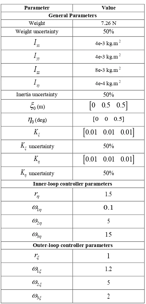
. These equations are mainly taken from references [6,28] and the interested reader is referred to them. In this paper, the parameters of three matrices J

( )

η

,Kξ, Kr and the mass

m

, are assumed to be uncertain but the variation boundaries are known. In a quadrotor configuration, the actuator system includes four independent rotors. Accordingly, the system is naturally underactuated and to control the platform completely, two states are used as virtual control inputs to control the other states. It means that the cascaded structure is chosen for handling the rotational and translational dynamics simultaneously. In this case, roll and pitch angles are selected as virtual control signals to regulate the tracking error of the horizontal components of position vectors

x t

( )

and

y t

( )

. Therefore, it is necessary to introduce a relative equation that can relate the desired value of attitude vector to the control force obtained from outer-loop controller utilized for regulating the position tracking error. The effects of actuator system can be described by Eq. (3) as follows:













1 2 3 4

t

x y z

u

f

l

f

l

f

c f

f



 

 



     



     



     



(3) (3)

where,

f

_i is the force generated by the

i

th component of the actuator system. Two parameters

l

and

c

are the moment arm and yaw moment factor which convert the force to moment vector. Therefore, F t

( )

in Eq. (1) is defined as follows.

 

_t

 

0

t

F t

R

u



 

 



_{ }

 

 

(4) (4)

It can be assumed that F t

_{( )}

includes three independent components described as T

( )

[

( )

]

x y z

F t = f t f t f t .

Therefore, the relation between these components and euler angles can be written as follows.

 





 





 

cos sin cos

sin sin

cos sin sin

sin cos

cos cos

x t

y t

z t

f t

u

f t

u

f t

u

 



 

  

















_

_





_



(5)

According to Eq. (5), if three components of the force vector are estimated from position controller loop, the desired values of roll and pitch angles can be determined accordingly. The explicit relation used to determine the desired value of roll and pitch angles is introduced in the following equation where, Sψ =sinψ and Cψ =cosψ .

 

_{ }

 

2 2 2

sin

tan

t x y z

x d y d

d

t

x d y d

d

z

u

f t

f t S

f t C

u

f t C

f t S

f t













_

_



_



_





_







(6) (6)

The controller design procedure for the system is divided into three steps according to a cascade architecture as follows: 1. Design the outer-loop controller for the path following problem assuming three independent control force components, and determine the desired value of the attitude vector.

2. Design the inner-loop controller to stabilize the attitude subsystem and track the desired value coming from the outer loop.

3. Prove the stability and boundedness of the cascade system considering the coupling terms between the inner and outer loops.

The remaining parts of this paper are organized to illustrate the above steps in more details.

3- Outer-Loop Contoller

(4)

154





9 1

‍

d

e



 















_



_





_

_







(7)

where, 3

d

ξ ∈ represents the desired path in three-dimensional space and 3

d

ξ ∈ is the corresponding velocity vector. According to Eq. (1), the following expression is suggested as the control effort applied to the system.





¨

1 1

c

f

m

K

mG

T

mT e K T e

T q



      



 









(8) (8)

This control scheme is composed of three segments. The first part corresponds to the left side of Eq. (1). The second part consists of two terms for regulating the error signal, and the third part is considered for disturbance attenuation and robustness against parameter uncertainty. In Eq. (8), Tξ is

defined as 3 9

1 2 3

[ ]

Tξ = Tξ T ξ T ξ ∈× composed of three

3 3× matrices. Using Eq. (8) as control force, and substituting it into Eq. (1), the position tracking error dynamics will be obtained from the following equation.

1

mT e K T e q T d

 



  

 

  (9) (9)

A more explicit form of Eq. (9) can be written as follows:





1 1 1 1

0 1 1 2 1 3 2 0

0 0

0 K

m

e T T I T T I T T T T e

I I



         

 



 

    

 



 

 

1 1

0 0

1 1

0 0

I I

m m

T q T w

   

   

 _ _  _ _

   

   

(10) (10)

where

1 2 3

9 9 0 0

0 0

T T T

T I I

I

ξ ξ ξ

ξ ×

 

 

=_ _∈

 

 

 , and 3

1

w T d= ξ ξ∈ .

Therefore, the error dynamics in Eq. (3) obtains a general form suitable for NLH∞ design [31] as follows.

 

e





f e

 



g e q k e w

 



  (11) (11)

Comparing Eqs. (10) and (11), the system matrices will be defined as follows in Eqs. (12) and (13).

 

1 1 1 1





0 1 1 2 1 3 2 0

0 0

0

K m

f e T T I T T I T T T T e

I I



          

_ 

 

    

 



 

 

(12)

   

1

0

1

0

0 I

m

g e

 

k e

 

T

















_

_













(13)

If the performance index is defined as W e q

ξ

ξ ξ

ζ =  _{ }  ,

where _W 1 12

ξ∈× is a weight matrix, then the NLH∞ can be stated as follows:

“Find the smallest value _γ*_≥₀_{such that for any}

γ γ

_≥ *

there exists a state feedback q q e t=

( )

ξ, , such that the

l

2 gain from

w

to ζ_ξ is less than or equal to

γ

, that is:”

2 2 2

2 2

0

‍‍

0

T T

dt

w

dt











(14) (14)

The internal term of integral expression of the performance index can be rewritten as Eq. (15):

2

2 T T T

e

q W W

q



   







_



_

 

_{ }

 

(15) (15)

Since _{W W}T

ξ ξ is symmetric and positive definite, it can be decomposed into 3 basic weight matrices as follows:

T

Q

S

W W

 

_S



_R



 





 







(16) (16)

where, Qξ and Rξ are two symmetric and positive definite matrices and_{Q S R S}1 T ₀

ξ − ξ ξ− ξ ≥ . To solve this problem, it is necessary to define a Lyapunov function V eξ

( )

ξ which

(5)

155

 

,

T

V V _{f e t} t e        

  (17)

     

1

 

2

1 1 _, _, _, _,

2

T

V V

k e t k e t g e t R g e t

e e                    _  _  _ _

 

_, 1 1



1



₀

2

T

T T T

V

g e t R S e e Q S R S e e                      (17) Theorem 1:

Suppose a Lyapunov function V e tξ

( )

ξ, =1₂e TTξ 0Tξ ξν

( )

e T eξ 0ξ ξ

where, ν

( )

eξ is a symmetric and positive definite matrix with the following structure:

 

0

0 mI

e

Y

X Y

X Y Z Y

        













_



_



_

_







(18)

where, _{X Y Z}_{, ,} 3 3

ξ ξ ξ∈× are three symmetric and positive definite matrices and _Z _{X Y X}1 ₂_X ₀

ξ − ξ ξ− ξ+ ξ ≥ . Using the proposed Lyapunov function, the HJB equation in Eq. (17) is constituted if the following holds.

0

2 2 2

2 0

T

Y X

T K T Y X Z X Q

X Z X

                  _  _  _    (19)





1 2

1 _{T T}

T

₍

_{S T R S T}

T

₎

T T

₀

      













(19) Proof:

To demonstrate the validity of Theorem 1, it is necessary to expand the HJB equation. From Eqs. (11) and (12), the Eqs. (20) to (24) can be concluded as follows.

0 0

0

T

mI

V

T

Y

X Y T e

e

X Y

Z Y

           







_

_



_



_



_

_









(20) (20)

Hence, the second term of the HJB is derived to be as Eq. (21):

 

,

T_V

f e t e        (21)









1 1

0 1 1 2

1 1

1 1 2

0

T T

K

e T T Y X T Y T

T X Y X Z T X Y T

                           _ _ _ _ 



















1

1 3 2 0

1

1 3 2

0

X T Y T T T e

X Z T X Y T T

                      _       _ (21)

After multiplying the inner matrices and simplifying the results, Eq. (21) can be written as follows:

 

1 1 1 2

2 1 2 2

3 1 3 2

,

2

T

T T

T T T

T T

V

_{f e t}

e

T K T

e T K T Y

T K T X

T K T

X Z

                           





























(22) 1 3 2 3 3 3 T T T

T K T

T K T e

T K T

         













(22)

Eq. (22) can be divided into two parts; the first one is composed of only X Y Zξ, ,ξ ξ and the second one is a quadratic

term based on matrix Tξ. Eq. (23) shows this expression as follows.

 

, 0 0 00

2 0

T

T T

V _{f e t e} _Y _X _{T K T e}

e _X _X _Z

                  _  _      __ _ _      (23) (23)

Since the term is a scalar and it equals to its transpose, Eq. (23) can be written as follows.

 

,

0

1 ₂

₂

2

0

T

T T

V

f e t

e

Y

X

e

T K T

Y

X

X Z e

X

X Z

(6)

156 The next two terms of HJB equation are evolved in Eq. (25).





1 2 2 1 2

1

2

1

2

T T T T T

V

k k

g R g

e

e T

I

R

T e

             



 





_





_







_

_





_











. (25)

1 1

T

T T T T

V

g R S e

e T R S e

e

            







(25)

After substituting Eqs. (24) and (25) into HJB equation and simplifying it, the following expression will be obtained.





1





2

0

2 2 2

2 0

1 ₀

T T

T

T T T

Y X

e T K T Y X Z X

X Z X

Q T T S T R S T e

              _                 _   _      _     (26) (26)

Therefore, if Eq. (19) is justified, the HJB equation will be satisfied using the proposed Lyapunov function. Accordingly, the optimal state feedback control law can be derived from Eq. (27) as follows:

* 1 T T

V

q

R S e g

e

      







 

_



_







(27)

the other hand, three matrices T T T1ξ, 2ξ, 3ξ used in Eq. (8) must be calculated to be used in the control law. To do this, it is necessary to solve Eq. (19) based on these matrices. The following shows an expanded expression of Eq. (19).

1 1 1 2 1 3

2 1 2 2 2 3

3 1 3 2 3 3

1 12 13

12 2 23

13 22 13

1 1 1

1 1 1 2 1 3

1 1 1

2 1 2 2 2

Γ

T T T

T T

T

Q

S R S

                                                          





























 













₃

1 1 1

3 1 3 2 3 3

1 1 1

1 1 1 2 1 3

1 1 1

2 1 2 2 2 3

1 1 1

3 1 3 2 3 3

1 1 1

1 1 1 2 1 3

1

2 1 2

T

T T T

T T T T T T

T T T

S R S

S R T

T R S

T

                                                                 





























 













1 1

2 2 3

1 1 1

3 1 3 2 3 3

2

0

2

0

T T T

T T T T T T

R S

T R S

Y

X

Y

X

Z

X

Z

                           

































_

_













(28) (28)

1 1 1 2 1 3

2 1 2 2 2 3

3 1 3 2 3 3

1 12 13

12 2 23

13 22 13

1 1 1

1 1 1 2 1 3

1 1 1

2 1 2 2 2

Γ

T T T

T T

T

Q

S R S

                                                          





























 













₃

1 1 1

3 1 3 2 3 3

1 1 1

1 1 1 2 1 3

1 1 1

2 1 2 2 2 3

1 1 1

3 1 3 2 3 3

1 1 1

1 1 1 2 1 3

1

2 1 2

T

T T T

T T T T T T

T T T

S R S

S R T

T R S

T

                                                                 





























 













1 1

2 2 3

1 1 1

3 1 3 2 3 3

2

0

2

0

T T T

T T T T T T

R S

T R S

Y

X

Y

X

Z

X

Z

                           

































_

_













(28) (28)

where, 2 1

1

Ãξ 2Kξ I Rξ

γ

−

= − + − _{. According to Eq. (28),}

1 , 2 , 3

T T Tξ ξ ξ can be calculated by solving at least 4 Riccati

equations as presented in the following procedure: 1. Calculate T₁ξ and T3ξ based on Eq. (29):

1 1 1

1TΓ 1 1 1 1T 1 1 1T 1T 0

T T Q S R S      S R T T R S       (29)

1 1 1

3TΓ 3 3 3 3T 3 3 3T 3T 0

T  T Q S R S  S R T T R S      

(29)

2. Calculate Xξ using Eq. (30):

1

1 3 13 1 3

1 1

1 3 1 3

Γ

T T

X

T

Q

S R S

S R T

T R S

       

     



 

 





(30) (30)

3. Calculate T2ξ using Eq. (31):

1

2 2 2 2 2

1 1

2 2 2 2

Γ

2

0

T T

T

Q

X

S R S

S R T

T R S

       

     



 







(31) (31)

Using matrices T T1ξ, 2ξ and T3ξ derived from above procedure and Eq. (27), the control law can be obtained as Eq. (32).





* 1 T

q

 

R S

 



T e

  (32) (32)

Hence, the optimal control force *

c

(7)

F. Rekabi et al., AUT J. Mech. Eng., 4(2) (2020) 151-168, DOI: 10.22060/ajme.2019.15561.5779 157 ¨ * d c

f



m





K





mG



(33)













1 1 1 1

1 2 1 1 1 1 1

1 1 1 1

1 3 1 2 1 2 2

1 1 1

1 3 1 3 3

1 1 1 T T T T

T T T K T T R S T

m

m T T T K T T R S T e

m

T K T T R S T

m                                                                (33)

Therefore, the control law can be stated in a Project Initiation Documentation (PID1_{) framework as Eq. (34):}

¨ *

d c

f



m





K





mG

(34)















_P _d _I ‍ _d _D _d



m K    K   dt K   

      

(34)

where, KPξ, KIξ and KDξ can be evaluated by comparing Eqs. (34) and (33) as mentioned in Eq. (35).













1 1 1 1

1 3 1 2 1 2 2

1 1 1

1 3 1 3 3

1 1 1 1

1 2 1 1 1 1 1

1

T P T I T D

K

T T

T K T

T R S

T

m

K

T K T

T R S

T

m

K

T T

T K T

T R S

T

m

                                      



_

_



_

_





_

_



(35) (35)

For more simplicity the following assumptions were made for weight matrices:

2 2 2

1 1 2 2 3 3

12 13 23

1 2 3

2

;

0

0 Q

I Q

I

Q

S

R

r I

ξ ξ ξ ξ ξ ξ ξ ξ ξ ξ ξ ξ ξ ξ

ω



=



₌





₌



₌



Therefore, the expression for controller gains reduce to the following form:

2

2 1 3 3

2 1 2

2 1 3

1

3 3

2

1 1

2

2 1 3

2 1

2

1

2

1

P I D

K

I

mr

K

m

K

I

K

mr

m

K

I

K

mr

m

                         



 



 



 



 







_





_



_















_



_











_

_





_

_

_

_

_



_

_



_

_





(36) (36) 1 Proportional-Integral-Derivative 2

2 1 3 3

2 1 2

2 1 3

1

3 3

2

1 1

2

2 1 3

2 1

2

1

2

1

P I D

K

I

mr

K

m

K

I

K

mr

m

K

I

K

mr

m

                         



 



 



 



 







_





_



_















_



_











_

_





_

_

_

_

_



_

_



_

_





(36) (36)

where, the parameters

ω ω ω

1ξ, ,ξ 3ξ and

r

ξ, are scalar

parameters and can be used for controller tunning. It must be mentioned that the final expression for the control law depends only on general parameters of the system, e.g., mass and speed. In addition, it does not depend on

γ

, and has an algebraic form for this special case.

4- Inner-Loop Controller

The design procedure for the inner-loop controller based on nonlinear H∞ is presented in this section. According to previous sections the rotational dynamic motion is affected by two sources of torque. Therefore, the net torque acting on the system can be introduced by the Eq. (37)

d

  

 

 

(37)

where,

τ



η is the control torque acting on the system and

d

η is the disturbance torque composed of both random and

stationary components. State equation for determining the control law is defined as Eq. (38).





‍

d d d

e

dt



 













_



_



_

_







(38) (38)

From the nonlinear rotational dynamics, the torque acting on the system can be derived from the control law according to Eq. (39) .

 

¨ m

 

,

J

C







 



  

(39)

 





1

1 m

,

1

T



J



T e C

 

T e

 

T u







(39)

Therefore, this control law can be divided in three parts: • First part is directly used for compensating the nonlinear dynamics,

• Second part is the regulator to decrease the error vector

e

η

and track the desired value when no disturbance influences the system,

(8)

158 control effort to compensate the disturbances affecting the system.

The matrix Tη appeared in the above equation can be written as Tη =[T₁η T₂η T₃η]. If this proposed control

scheme is used to track the desired attitude, the dynamic equation describing the rotational motion will be summarized as follows.

 

m

 

,

J



T e C

 



 

T e u d

 

 

 (40) (40)

where,

( )

1

( )

1

dη =J

η

T Jη −

η

dτ. In fact this equation

represents the error dynamics and based on this equation the nonlinear H∞ controller design can be introduced as follows: “Determining the control law u t

( )

which can reduce the 2

l

gain from the cost function

ζ

η to the disturbance signal

energy less than a defined value

γ

. The cost function

ζ

η is

introduced as equation”:

T T T

e

u W W

u



   







_



_

 

_{ }

 

(41) (41)

and the term _{W W}T

η η which is a symmetric and positive

definite matrix, can be written as Eq. (42).

1

, 0, 0

T

Q S

W W _S _R Q S R S R

     

 



 

_ _   

  (42) (42) If the error dynamics is rearranged in the following form:

 

,

 

,

 

,

e





f e t

 



g e t u k e t d

 



   (43) (43)

then, a norm solution can be found satisfying Eq. (44).

 

,

T

V

f e t

t

e

 

  







 

_,

1

1 

1



2

T

T T T

V

g e t R S e

e Q S R S e

e



           

 











   

2

1

1 _,

_,

2

T

V

k e t k e t

e



   













 

_

_

_



_





(44)

 

_,

1 T

 

_,



V

₀

g e t R g e t

e



    















_



_









(44)

For every γ > σ_max

( )

_R_η ≥₀, where

σ

_max indicates the

maximum singular value, the optimal control law can be expressed as Eq. (45).

   

* 1 T T

_,

V e t

,

u

R S e g e t

e

      







_





_

 













(45) (45)

Theorem 2:

Suppose a Lyapunov function

( )

, 1₂ T 0T

( )

0

V e tη η = e Tη η η

ν

e T eη η η where,

ν

( )

e

η is a

symmetric and positive definite matrix with the following structure:

 

0  

0

0 J

e

Y

X

Y

X

Y Z Y

    

   















_



_



_

_







(46) (46)

where, _{X Y Z}_{, ,} 3 3

η η η∈× are three symmetric and positive

definite matrices and _Z _{X Y X}1 ₂_X ₀

η− η η− η+ η≥ . This

Lyapunov function constitutes the HJB equation in Eq. (44) if the expression Eq. (47) holds.

0

2 2 2

2 0

T

Y X

T K T Y X Z X Q

X Z X

 

       

  

 

 

 _  _

 _ 

 

(47)





1 2

1 _{T T}

T

₍

_{S T R S T}

T

₎

T T

₀

      













(47)

Proof:

The proof of this theorem can be found in reference [19]. According to reference [24] and making simplifying assumptions similar to previous section, the control law for the rotational subsystem can be described by Eqs. (48) to (53).





* 1 T

u

 

R S

 



T e

  (48)(48)

(9)

159

 

¨





*

_,

d

d m d d

J

C







 



  

(49)



J

 



d





K

D

K

P

K e

I







(49)

For convenience, the structure of the matrices Qη, Rη and Sη were chosen as follows.

2 1

2 2

2 3

2

0

0 ,

0

0 ,

0 .

0 I

Q

I

R

r I S



 



  











 











 

 



_{  }

 

 

(50) (50)

As a result, the gain matrices can be calculated from the Eqs. (51) to (53).

2

2 1 2

2

1 1

2

P

K



I

  

I



 



 









(51)

J C

1 m

_r

1

₂

I













_





_





(51)

2

2 1 2 1

2 1

2 ₁

D m

K

I J

C

I

r

  



 



 

















_





_





(52) (52)

2 1

1

I m

K

J C

I

r



 













_





_





(53) (53)

Although a threshold

γ

was defined in the control design and appeared in the first expressions of the control law, it can be seen that the final expression for the gain matrices is independent from this parameter and therefore it can be used as a general expression for compensating the disturbance effects.

5- Stability Analysis

In the previous sections, two control algorithms were developed for position tracking and attitude stabilization based on Eqs. (1) and (2). In dynamic modeling, it was mentioned that the position tracking subsystem uses three

independent force components to regulate the tracking error signal. Although there exists an explicit relation between three force components and euler angles based on Eq. (6), but the attitude tracking stability can not guarantee the stability of the overall cascade system solely. In fact, the error dynamic models for inner and outer loops have a coupling term which affects the stability of the cascade system. To analyze the stability behavior Eq. (54) is used which considers the coupling terms between two subsystems.

   

 

   

 

Δ

f

e

f e

g e q k e w

e

f e

g e u k e d

       

      

 













(54) (54)

where, f f g g kξ, , , ,η ξ η ξ and

k

η have the same

definitions as stated in Sections 3 and 4. Ä_f is the coupling term between inner and outer loop and is equal to

1

0 1 Δ

1 Δ

0

f

m

T



T f



 

 



_{ }

 

 

(55)

where, f_Ä=R_t

( ) ( )

η

F t −f_c and can be obtained from Eq. (56).



 





 





 



Δ

d d d d d

t d d d d d

d d

f

C S C S S C S C S S

u C S S S C C S S S C

C C C C

                       



    

 _ _ _ 

 

  

 

(56)

Following lemmas are introduced to analyze the stability of cascade NLH∞ system for Eq. (54) based on [28, 30-31]. Lemma 1

If there exists a proper solution V ≥0 for HJB equation and the system x f x=