__________
* Corresponding author
E-mail addresses:[email protected](I. Khosravi);[email protected](M. Momeni)
Presenting an extended evaluation framework for building detection
algorithms using high spatial resolution images
Iman Khosravi*, Mehdi Momeni
Department of Surveying Engineering, Faculty of Civil Engineering and Transportation, University of Isfahan, Isfahan, Iran
Article history:
Received:02December 2016, Received in revised form: 22March2017,Accepted:22April2017
ABSTRACT
This paper aims to provide an extended evaluationframework for building detection algorithms using a diverse set ofHigh Spatial Resolution (HSR) images. The HSR images utilized in this paper were chosen from different places anddifferent sensors, and based on several important challenges in an urban area such as building alignment, density, shape, size, color, height, and imaging angle.The classical evaluation metricssuch as detection rate, reliability, false positive rate, and overall accuracy only demonstrate the performance evaluation of an algorithm in relation to the buildings and cannot interpretthe mentioned challenges. The extended evaluation framework proposed in this paper composed several extended metrics for performance evaluation of building detection algorithms in relation to these challenges in addition to the classical metrics. The paperintends to declarethat the success or failure metrics of a building detection algorithm can have more varieties. In fact, a building detection algorithm may be successful at one or several metrics, whilstitmay be unsuccessful at the other metrics.
S
KEYWORDS
Evaluation
Accuracy
Error matrix
Building detection
High spatial resolution images
1. Introduction
In the last two decades, the detection of buildings from High Spatial Resolution (HSR) images has received much attention for many applications in Earth Observation and Geomatics Engineering (EOGE) such as map updating, urban planning, 3D modeling, disaster management, and change detection. Until now, many building detection algorithms were proposed in the literatures. The performance evaluation of these algorithms is an important task of the studies (Khoshelham et al., 2010). Usually, several famous and common metrics extracted from the error matrix were used for evaluation of the algorithms such as Detection Rate (DR), Reliability (R), False Positive Rate (FPR), and Overall Accuracy (OA). Their meanings and calculation methods can be found in some studies (e.g.
Khoshelham et al., 2010 ; Ghanea et al., 2014 ; Khosravi et al., 2014). Up to now, the HSR images used in the building
building were diverse in terms of
studies detection
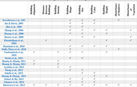
alignment, distance between buildings, building density, building shape, building size, building color, and building height. In addition to the challenges mentioned above, the presence and disturbance of shadows and vegetation areas can be observed in the proximities of buildings (see Table 1). All of these challenges do not exist in the images of the previous studies. Furthermore, the classical evaluation
and OA DR, R, FPR,
metrics, i.e. , only explain the
performance evaluation of algorithms in relation to buildings (Khoshelham et al., 2010). Nonetheless, the effect of some challenges is neglected in these metrics. For example, the classical metrics are not able to indicate the evaluation of algorithms in relation to imaging angle or they cannot demonstrate how much the vegetation, shadow or non-building areas can be removed by algorithms. In fact, they cannot point out whether an algorithm is able to
72 eliminate all the vegetation, shadow or non-building areas
from image or not. The main objective of this paper is to introduce a diverse set of HSR images based on all the challenges mentioned above (see Table 1) and then, to provide several quantitative metrics for performance evaluation of building detection algorithms in relation to these Challenges. The next sections of the paper are as follows. In Section 2, a diverse set of HSR imagery is introduced and then several evaluation metrics are provided based on them. These metrics and classical metrics establish an extended evaluation framework. In Section 3, the extended framework is applied in order to compare three building detection algorithms. This section indicates that the success or failure metrics of a building detection algorithm can have a wide range and an algorithm may be more successful or unsuccessful than the other algorithms at one or several evaluation metrics. Finally, Section 4 contains the conclusion of the paper.
2. Methodology: Extending evaluation framework
2.1 A diverse set of HSR images
Twelve regions were chosen from different places and different sensors (see Figures 1). Regions 1-(a), (e), (f), (g),
(h), (i), (k), and (l) were the pan-sharpened QuickBird images (0.6m resolution) and region 1-(j) was the pan-sharpened GeoEye-1 image (0.5m resolution at stereo mode) of the city of Isfahan. Region 1-(d) was the pan-sharpened GeoEye-1 image (at nadir mode) of the city of Tehran and regions 1-(b) and 1-(c) were the pan-sharpened QuickBird images of the city of Ankara. All the images were pre-processed by histogram stretching to enhance. There were many different urban objects such as roads, yards, shadows, vegetation, green spaces, bare land, and the most important feature, i.e. buildings in these images. They can be thus considered as a diverse set of HSR images in terms of "building alignment and distance, density, shape, color and reflectance, the presence of shadow and vegetation, variation of buildings height, and imaging angle". Based on the most prominent property of each region, twelve regions are categorized as follows:
- Regions (a) and (b) have the buildings with regular alignment, where the former has blocks of buildings, while the latter has single buildings. By contrast, region (c) has the buildings with irregular alignment.
Table 1. The challenges used in previous building detection studies
B u il d in g A li g n me n t D ist a n ce B et w ee n B u il d in g s B u il d in g D en si ty B u il d in g S h a p e B u il d in g S iz e B u il d in g C o lo r B u il d in g Hei g h t D ist u rb a n ce o f S h a d o w s D ist u rb a n ce o f V eg et a ti o n
Benediktsson et al., 2003
Jin & Davis, 2005
Hui et al., 2006
Zhang et al., 2006
Huang et al., 2008
Hester et al., 2008
Khoshelham et al., 2010
Bouziani et al., 2010
Dalla Mura et al., 2010
Taubenbuck et al., 2010
Myint et al., 2011
Huang & Zhang, 2011
Huang & Zhang, 2012
Aytekin et al., 2012
Meng et al., 2012
Salehi et al., 2012
Huang & Zhang, 2013
Sebari & He, 2013
Ghanea et al., 2014
72
(a) (b) (c)
(d)
(e) (f) (g)
(h)
(i) (j) (k)
(l)
Figure1.A diverse set of HSR images applied in this paper, (a) Regular blocks,(b) Regular single,(c) Irregular,(d) Positional dense,(e) Ragged edge,(f) Straight edge,(g) Troublesome shadows,(h) Troublesome vegetation,(i) Variation of height,(j) Oblique image,(k)Similar
reflectance & blocks,(l) Similar reflectanceandsingle
- The building density of region (d) is relatively high. - Some buildings of region (e) have the ragged edges, whereas all the buildings of region (f) have straight edges.
- The troublesome urban objects, i.e. shadow and vegetation areas can be observed in proximities of buildings in regions (g) and (h), respectively.
- The buildings of region (i) have diverse height. The image of region (j) is an oblique image unlike the other regions.
- Finally, there is similar reflectance (or low contrast) between the building and non-building areas in regions (k) and (l), where the former has blocks of buildings and the latter has single buildings.
2.2 Classical evaluation metrics
The classical evaluation metrics such as DR, R, FPR, and OA are defined as follows where the reference data is the buildings image extracted from a digital map (Khoshelham et al., 2010):
FN TP
TP DR
(1)
FP TP
TP R
(2)
FP TN
FP FPR
(3)
FN FP TN TP
TN TP OA
(4)
TP and TN are the numbers of pixels correctly detected as building and non-building, respectively. FP is the number of non-building pixels detected as building and FN is the number of building pixels detected as non-building (Khosravi et al., 2014). FPR represents the commission error of buildings produced by algorithm. A higher DR
value indicates the high efficiency of an algorithm in the detection of building. A higher R and a lower FPR implies the reliability of the produced results (Khoshelham et al., 2010).
2.3 Extended evaluation metrics
72 2.3.1 Building alignment
When the building alignment is diverse such as regions (a), (b) and (c), how much building areas can be detected by algorithm. Therefore, Building Detection Rate (BDR) index can be a proper metric for performance evaluation of algorithm in relation to building alignment. It is defined by (Khoshelham et al., 2010) as DR index Eq. (1) where buildings image extracted from a digital map is considered as the reference data. Thus,IRB, IRSand IIR, i.e. evaluation metrics, which consider building alignment, are defined as follows:
DR BDR I
I
IRB RS IR (5)
2.3.2 Building density
At a dense urban area such as region (d), the amount of building areas can be detected by algorithm. Thus for the performance evaluation of algorithm in relation to building density, again BDR index is a good metric, where the reference data is the buildings image extracted from a digital map. IPD, the evaluation index which considers the building density is defined as follows:
BDR
IPD (6) Generally speaking, the DR metric can talk about the sensitivity of an algorithm in relation to building alignment and density, in addition to the rate of building regions detected by that algorithm.
2.3.3 Building edges
At region (e) or (f), the amount of ragged or straight edges can be detected by algorithm. In these cases, the Ragged Edges Detection Rate (REDR) and the Straight Edges Detection Rate (SEDR) are defined as follows:
TRE DRE
REDR (7)
TSE DSE
SEDR (8)
DRE and DSE are the numbers of detected ragged and straight edges pixels, respectively. TRE and TSE are the total ragged and straight edges pixels at regions (e) and (f), respectively. Manually ragged edges image of region (e) and manually straight edges image of region (f) are considered as the reference data. Thus, two metrics, IREand
SE
I , which consider the building edges can be defined as:
REDR
IRE (9) SEDR
ISE (10)
The performance of an algorithm is directly dependent on
REDR and SEDR values. 2.3.4 Troublesome objects
Where shadow or vegetation areas are the proximities of buildings such as region (g) or (h), the amount of the shadow or vegetation areas are removed by algorithm. In these cases, the number of shadow and vegetation pixels that have been wrongly detected as buildings are computed in regions (g) and (h), respectively. Thus, the False Shadow Detection Rate (FSDR) and the False Vegetation Detection Rate (FVDR) are defined as follows:
TS FDS
FSDR (11)
TV FDV
FVDR (12)
FDS and FDV are the false number of the detected shadow and vegetation pixels as buildings and TS and TV are the total shadow and vegetation pixels at regions (g) and (h), respectively. Manually shadow image of region (g) and manually vegetation image of region (h) are considered as the reference data. Two metrics, i.e. IFSandIFV, which indicate the ability of an algorithm in eliminating shadow and vegetation areas can be defined as follows:
FSDR
IFS1 (13)
FVDR
IFV1 (14) In fact, the efficiency and reliability of an algorithm have reverse dependency with the FSDR and FVDR values. 2.3.5 Building height
At an urban area with a variety of buildings heights such as region (i), the more building areas an algorithm is able to detect, the more efficient the algorithm is. Thus, BDR index seems to be a proper metric for performance evaluation of algorithm in relation to building height. IVH, the evaluation index, which considers building height, is defined as follows:
BDR
IVH (15) 2.3.6 Imaging angle
03
TSV FDSV
FSVDR (16)
where, FDSV is the false number of detected side view pixels as buildings and TSV is the total side view pixels at region (j). In addition, manually side view image of region (j) is considered as reference data. IOI, which indicates the ability of algorithm in eliminating the side view areas, is defined as follows:
FSVDR
IOI 1 (17) here, the efficiency and reliability of an algorithm have reverse dependency with the FSVDR value. A lower
FSVDR implies the high efficiency and reliability of an algorithm in the detection of buildings, whilst its high value indicates the inability of that algorithm in eliminating all side view areas.
2.3.7 Similar reflectance
Where there is a similar reflectance between building and non-building areas such as regions (k) and (l), the amount of non-building areas are removed by algorithm. In these cases, the False Non-Building Detection Rate (FNBDR), i.e. the number of non-building pixels that have been wrongly detected as buildings, should be computed as follows:
TNB FDNB
FNBDR (18)
FDNB is the false number of detected non-building pixels and TNB is the total non-building pixels at regions (k) and (l). Reference data is the manually non-building image of these regions. Thus, ISRB (blocks) and ISRS (single), which indicate the ability of algorithm in eliminating the non-building areas, can be defined as follows:
FNBDR I
ISRB SRS 1 (19) Similar previous index, the efficiency and reliability of an algorithm have reverse dependency with the FNBDR value. Consequently, at an urban area with similar reflectance between building and non-building areas, a lower FNBDR
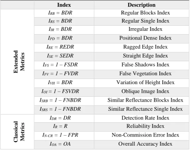
implies the high efficiency and reliability of the algorithm in the detection of buildings and its high value indicates the inability of that algorithm in eliminating all adjacent non-building areas. All the extended metrics mentioned above besides the classical metrics establish an extended evaluation framework. The metrics of this framework and their descriptions are shown in Table 2.
3. Experiment and discussion
3.1 An overview of three building detection algorithms
For experiment, we selected three recent studies as representatives of all algorithms which had the attractive and complex structures and approximately covered all the processing tricks for building detection using only HSR
images. The first two algorithms are based on the work of )Ghanea et al., 2014 ; Aytekin et al., 2012), where the former is the combination of clustering, and segmentation methods (CS), and the latter is the combination of spectral metrics, clustering, and the morphological methods (ICM). The final algorithm is an Object-Based image Classification (OBC).
3.1.1 Algorithm CS (Clustering and Segmentation)
The algorithm CS presented by (Ghanea et al., 2014)
included these steps (Figure 2): in the first step, a k-means clustering (K=2) was applied to the original image to convert it to a binary image, consisted of the semi-building layer and the non-building layer. Then a closing morphological operator was used to cover the small non-building areas surrounded by the semi-non-building layer. Afterwards, a Fuzzy C-Means (FCM) clustering was applied to the semi-building layer to split it into several clusters. Each cluster was decomposed into independent areas using a connected component labelling process. After the FCM clustering, the small pseudo-building areas were eliminated using an area thresholding. The area of the smallest building was considered as the threshold value. Then, a region-growing segmentation was applied to eliminate the large pseudo-building areas. The variance and the area of the segments were used as the similarity criterion for segmenting. The threshold value for area was the area of the largest building. In addition, the variance of all points belonging to each segment at the previous step was considered as the variance threshold for that segment. The holes of the building areas were closed using a filling morphological operator and finally, only the building areas were remained in the image.
03 Thus, man-made areas (include mainly the building
rooftops and roads) were extracted after the classification of the vegetation and shadow areas. Afterwards, a modified version of the thinning algorithm (Aytekin et al., 2012) was applied to each segment and then the main roads were separated from other segments using Otsu's thresholding. Next, the small artifacts were filtered using the principle component analysis and a morphological operator such as (Gonzales et al., 2004). Finally, only the building areas were remained in the image.
3.1.3 Algorithm OBC (Object-Based Classification) The most important step in algorithm OBC was segmentation. It used a multiresolution segmentation belonging to eCognition Developer software (eCognition User Guide, 2012). The multiresolution segmentation needed three main parameters to be tuned: scale, shape, and compactness (Baatz & Schape, 2000). After producing the segments, the classes such as roads, vegetation, shadows, bare land, and buildings were defined and the training samples were then collected for each class. Then, the mean values for NDVI, green and brightness, area, length to width ratio, rectangular fit, and shape index were selected as object attributes. Finally, the algorithm determined the label of each segment using the nearest neighbor classifier based on fuzzy logic and then, buildings were separated from the classified image (Figure 4).
3.2 Evaluation results
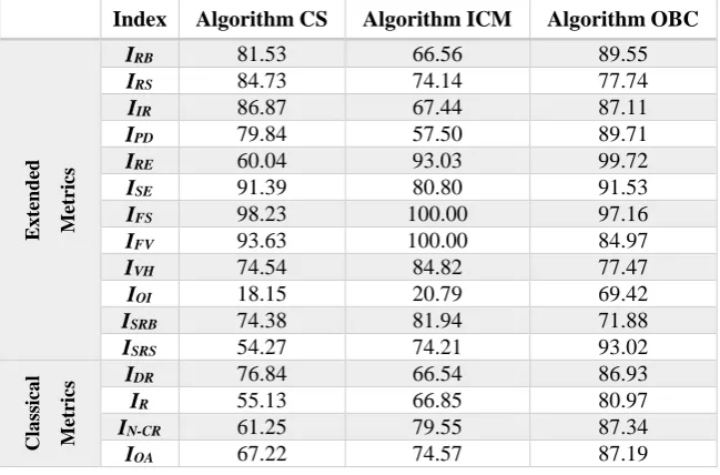
The comparative evaluation results of the three algorithms using the extended framework are shown in Table 3 and also Figure 5. The results are presented in two distinct sections: by the classical metrics and by the
extended metrics.
3.2.1 Comparative evaluation by classical metrics
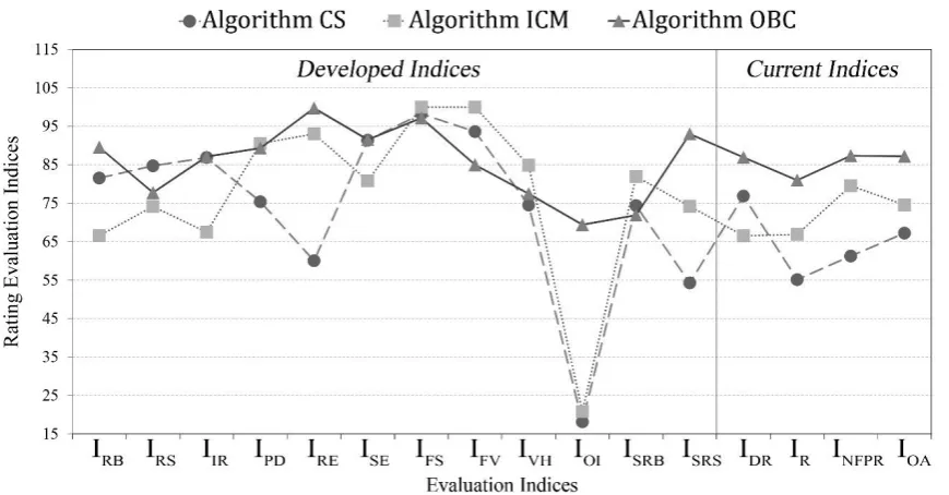
From Table 2, the IDRrate of algorithm OBC is around 87% which is 10% and 20% higher than the ones of algorithms CS (77%) and ICM (67%), respectively. In addition, the IR rate of algorithm OBC (81%) is 26% and 14% higher as compared to the algorithms CS (55%) and ICM (67%), respectively. Moreover, the commission error of algorithm OBC is around 26% which is 7% lower than the ones of algorithms CS and ICM. In addition, the overall accuracy of algorithm OBC is 20%, which is 12% higher as compared to the two other algorithms. These results can be seen in the right of the vertical dotted line of Figure 5. Therefore, it can be concluded that algorithms OBC is more efficient and dependable than the algorithms CS and ICM. This issue may be due to the use of segments (instead of single pixels) and also non-spectral features at the object-based process. In comparison between the two non-object-based algorithms, it can be seen that the IDRrate of algorithm CS is 76% which is around 9% higher than algorithm ICM with the IDRvalue of 67%. Conversely, the
R
I value of algorithm ICM (67%) is around 12% higher than the ones of algorithm CS (55%). In addition, the commission error of algorithm ICM (20%) is 19% lower than the ones of algorithm CS (39%). Thus, these results represent that although algorithm CS is more efficient than algorithm ICM in the detection of building, nevertheless algorithm ICM is more dependable than algorithm CS. 3.2.2 Comparative evaluation by developed metrics
Although, algorithm OBC was more successful than the other two algorithms at all classical metrics, however it may Table 2. The developed evaluation framework for building detection algorithms
Index Description
Ex
te
n
d
ed
Metr
ics
IRB = BDR Regular Blocks Index
IRS = BDR Regular Single Index
IIR = BDR Irregular Index
IPD = BDR Positional Dense Index
IRE = REDR Ragged Edge Index
ISE = SEDR Straight Edge Index
IFS = 1 – FSDR False Shadows Index
IFV = 1 – FVDR False Vegetation Index
IVH = BDR Variation of Height Index
IOI = 1 – FSVDR Oblique Image Index
ISRB = 1 – FNBDR Similar Reflectance Blocks Index
ISRS = 1 – FNBDR Similar Reflectance Single Index
Cla
ss
ica
l
Metr
ics
IDR = DR Detection Rate Index
IR = R Reliability Index
IN-CR = 1 – FPR Non-Commission Error Index
07 the
metrics. In developed
at some be unsuccessful
following, the results of comparative evaluation by developed metrics are provided in detail:
- Building alignment and distance (IRB,IRSand IIR): From Table 2 and Figure 5, algorithm ICM is the most unsuccessful at three metrics IRB, IRSand IIR. Conversely, algorithm OBC is the most successful at two metrics IRB (90%) and IIR (93%); and algorithm CS is the most successful at IRS (85%) which is 7% higher than the ones of algorithm OBC. These cases indicate "where there are blocks of buildings, algorithm OBC is more successful than the other two algorithms, and algorithm CS is more
buildings single
there are
successful, when while the
algorithm of
performance ICM is lowest in the two
conditions".
- Building positional density (IPD): In the dense urban area, algorithms OBC could be more successful than the other two algorithms with the IPDrate of 90% versus 80% and 58%. In addition, algorithm CS was more efficient than algorithm ICM in the detection of buildings from a dense area.
- Building Edge (IREandISE): From Table 2, theIRE
and ISErates of algorithm OBC are the most (around 100% and 92%), whereas the IREof algorithm CS is the lowest (60%) and the ISErate of algorithm ICM is the lowest (81%).
- Troublesome Objects (IFSandIFV): Notable results of Table 2 are related to IFSand IFVmetrics. As it can be seen, the IFSand IFVrates of algorithm ICM have been 100% which are better than the other two algorithms. In
addition, algorithm CS is more successful than algorithm OBC at these two metrics. These two cases indicate that "algorithm ICM is more successful and dependable than the other algorithms (especially object-based method) in
shadow and vegetation areas
eliminating all from the
regions (g) and (h), respectively. Conversely, algorithm OBC is the most unable algorithm in eliminating all shadow and vegetation areas".
- Building Height (IVH): Similar to the two previous metrics, the IVHrate of algorithm ICM is 85% which is better as compared to the other algorithms even object-based method, whereas, the one of algorithm CS is the lowest with the rate of 75%. Thus, "in an urban area with variation of building height, algorithm ICM is the most successful and algorithm CS is the most unsuccessful in the detection of buildings".
- Imaging Angle (IOI): The IOIrate of algorithm OBC is 69% which is much better as compared to the other two algorithms (around 48–51% higher). This case indicates "algorithm OBC is much more successful and dependable than the other two algorithms in eliminating the side view areas of region (j), while algorithm CS has the lowest efficiency".
- Similar Reflectance (ISRBandISRS): The ISRBrates of algorithms ICM (82%) and CS (74%) are more than the ones of algorithm OBC (72%). Conversely, the ISRSrate of algorithms OBC (93%) is much more as compared to the algorithms ICM (74%) and CS (54%).
(a) (b) (c)
(d) (e) (f)
Figure2.The procedure of algorithm CS,(a) Binary image produced by k-means clustering with k = 2,(b) Post-processing using a closing morphological operator,(c) Semi-building layer clustering by FCM,(d) Eliminating the small pseudo-building areas,(e) Region-growing
00 (a) (b) (c)
(d) (e) (f)
Figure 3. The procedure of algorithm ICM, (a) Masking vegetation, (b) Masking shadows, (c) Man-made image, (d) Masking roads, (e) Filtering the artifacts, (f) The final result of building detection
(a) (b) (c)
Figure 4. The procedure of algorithm OBC, (a) Multiresolution segmentation, (b) Classified image, (c) The final result of building detection
Table 3. Comparative evaluation results of algorithms using the developed framework
Index Algorithm CS Algorithm ICM Algorithm OBC
Ex
te
n
d
ed
Metr
ics
IRB 81.53 66.56 89.55
IRS 84.73 74.14 77.74
IIR 86.87 67.44 87.11
IPD 79.84 57.50 89.71
IRE 60.04 93.03 99.72
ISE 91.39 80.80 91.53
IFS 98.23 100.00 97.16
IFV 93.63 100.00 84.97
IVH 74.54 84.82 77.47
IOI 18.15 20.79 69.42
ISRB 74.38 81.94 71.88
ISRS 54.27 74.21 93.02
Cla
ss
ica
l
Metr
ics
IDR 76.84 66.54 86.93
IR 55.13 66.85 80.97
IN-CR 61.25 79.55 87.34
03 Figure 5. Comparative evaluation using the developed framework between three algorithms
It can be concluded that "algorithms ICM and CS are the most successful in eliminating the non-building areas where there is similar reflectance between the building blocks and non-building areas; while algorithm OBC is the most successful in eliminating the non-building areas, where there is a similar reflectance between single building and non-building areas."
4. Conclusion
This research study which presented an extended evaluation framework indicated that the success or failure metrics of a building detection algorithm can have a wide range. In the proposed framework, the quantitative metrics such as the evaluation metrics in relation to the detection of buildings from a dense urban area, from a region with regular or irregular alignment, from a region with variation of building height, moreover in relation to the eliminating shadow, vegetation, side view and non-building areas were presented. The conclusion of the comparison between the three building detection algorithms using the proposed framework was as follows: Algorithm ICM was more successful than the other two algorithms in eliminating all the troublesome shadow, vegetation and non-building areas (in an urban area with building blocks) and the detection of building areas in a region with variation of height, (i.e. at 4 metricsIFS,IFV, IVHandISRB). Moreover, at 6 other metrics (IRE,IOI,ISRS,IR,INCRandIOA), it was more successful than algorithm CS. Finally, it was the most unsuccessful at 6 remaining metrics (IRB,IRS,IIR,IPD,ISE and IDR). The algorithm OBC was the most successful at 11 metrics (IRB,IIR,IPD,IRE,ISE,IOI,ISRB,IDR,IR,
CR N
I and IOA), it was especially more successful in
eliminating the side view and non-building areas (in an urban area with single buildings). However, at 3 metrics (IFS,IFVand ISRB), it was the most unsuccessful. In other words, algorithm OBC was unable to eliminate the troublesome shadow, vegetation areas and non-building areas (at an urban area with building blocks). Finally, it can be concluded that a building detection algorithm may be successful at one or several metrics, while it may fail at the other metrics.
References
Aytekın, Ö., Erener, A., Ulusoy, İ., & Düzgün, Ş. (2012). Unsupervised building detection in complex urban environments from multispectral satellite imagery. International Journal of Remote Sensing, 33(7), 2152-2177.
Baatz, M. (2000). Multiresolution segmentation: an optimization approach for high quality multi-scale image segmentation. Angewandte geographische informationsverarbeitung, 12-23.
Benediktsson, J. A., Pesaresi, M., & Amason, K. (2003). Classification and feature extraction for remote sensing images from urban areas based on morphological transformations. IEEE Transactions on Geoscience and Remote Sensing, 41(9), 1940-1949.
Bouziani, M., Goita, K., & He, D. C. (2010). Rule-based classification of a very high resolution image in an urban environment using multispectral segmentation guided by cartographic data. IEEE Transactions on Geoscience and Remote Sensing, 48(8), 3198-3211. Dalla Mura, M., Benediktsson, J. A., Waske, B., &
03 Transactions on Geoscience and Remote Sensing,
48(10), 3747-3762.
eCognition Developer 8.7.2 User Guide. 2012
Ghanea, M., Moallem, P., & Momeni, M. (2014). Automatic building extraction in dense urban areas through GeoEye multispectral imagery. International journal of remote sensing, 35(13), 5094-5119.
Gonzalez R.C, Woods R.E, Eddins S.L. Digital Image Processing Using MATLAB, 2nd ed. Prentice-Hall, Inc, 2004.
Hester, D. B., Cakir, H. I., Nelson, S. A., & Khorram, S. (2008). Per-pixel classification of high spatial resolution satellite imagery for urban land-cover mapping. Photogrammetric Engineering & Remote Sensing, 74(4), 463-471.
Lu, Y. H., Trinder, J. C., & Kubik, K. (2006). Automatic building detection using the Dempster-Shafer algorithm. Photogrammetric Engineering & Remote Sensing, 72(4), 395-403.
Huang, X., & Zhang, L. (2011). A multidirectional and multiscale morphological index for automatic building extraction from multispectral GeoEye-1 imagery. Photogrammetric Engineering & Remote Sensing, 77(7), 721-732.
Huang, X., & Zhang, L. (2013). An SVM ensemble approach combining spectral, structural, and semantic features for the classification of high-resolution remotely sensed imagery. IEEE transactions on geoscience and remote sensing, 51(1), 257-272.
Huang, X., Zhang, L., & Li, P. (2008). Classification of very high spatial resolution imagery based on the fusion of edge and multispectral information. Photogrammetric Engineering & Remote Sensing, 74(12), 1585-1596. Hunag X, Zhang L. Morphological building/shadow index for building extraction from high–resolution imagery over urban areas, IEEE Journal of Selected Topics in Applied Earth Observations and Remote Sensing, vol. 5, no. 1, pp. 161–172, February 2012. Jin, X., & Davis, C. H. (2005). Automated building
extraction from high-resolution satellite imagery in urban areas using structural, contextual, and spectral information. EURASIP Journal on Advances in Signal Processing, 2005(14), 745309.
Khoshelham, K., Nardinocchi, C., Frontoni, E., Mancini, A., & Zingaretti, P. (2010). Performance evaluation of automated approaches to building detection in multi-source aerial data. ISPRS Journal of Photogrammetry and Remote Sensing, 65(1), 123-133.
Khosravi, I., Momeni, M., & Rahnemoonfar, M. (2014). Performance evaluation of object-based and pixel-based building detection algorithms from very high spatial resolution imagery. Photogrammetric Engineering & Remote Sensing, 80(6), 519-528.
Meng, X., Currit, N., Wang, L., & Yang, X. (2012). Detect
residential buildings from lidar and aerial photographs through object-oriented land-use classification. Photogrammetric Engineering & Remote Sensing, 78(1), 35-44.
Myint, S. W., Gober, P., Brazel, A., Grossman-Clarke, S., & Weng, Q. (2011). Per-pixel vs. object-based classification of urban land cover extraction using high spatial resolution imagery. Remote sensing of environment, 115(5), 1145-1161.
Salehi, B., Zhang, Y., Zhong, M., & Dey, V. (2012). Object-based classification of urban areas using VHR imagery and height points ancillary data. Remote Sensing, 4(8), 2256-2276.
Sebari, I., & He, D. C. (2013). Automatic fuzzy object-based analysis of VHSR images for urban objects extraction. ISPRS Journal of Photogrammetry and Remote Sensing, 79, 171-184.
Taubenböck, H., Esch, T., Wurm, M., Roth, A., & Dech, S. (2010). Object-based feature extraction using high spatial resolution satellite data of urban areas. Journal of Spatial Science, 55(1), 117-132.