https://doi.org/10.5194/gmd-12-3835-2019 © Author(s) 2019. This work is distributed under the Creative Commons Attribution 4.0 License.
Improved methodologies for Earth system modelling of atmospheric
soluble iron and observation comparisons using the Mechanism of
Intermediate complexity for Modelling Iron (MIMI v1.0)
Douglas S. Hamilton1, Rachel A. Scanza2, Yan Feng3, Joseph Guinness4, Jasper F. Kok5, Longlei Li1, Xiaohong Liu6, Sagar D. Rathod7, Jessica S. Wan1, Mingxuan Wu6, and Natalie M. Mahowald1
1Department of Earth and Atmospheric Science, Cornell University, Ithaca, NY, USA
2Atmospheric Sciences and Global Change Division, Pacific Northwest National Laboratory, Richland, Washington, USA 3Environmental Science Division, Argonne National Laboratory, Argonne, IL, USA
4Department of Statistics and Data Science, Cornell University, Ithaca, NY, USA
5Department of Atmospheric and Oceanic Sciences, University of California, Los Angeles, CA 90095, USA 6Department of Atmospheric Science, University of Wyoming, Laramie, WY, USA
7Department of Civil and Environmental Engineering, University of Illinois at Urbana–Champaign, Urbana, IL, USA Correspondence:Douglas S. Hamilton ([email protected])
Received: 28 March 2019 – Discussion started: 6 May 2019
Revised: 29 July 2019 – Accepted: 30 July 2019 – Published: 2 September 2019
Abstract. Herein, we present a description of the Mecha-nism of Intermediate complexity for Modelling Iron (MIMI v1.0). This iron processing module was developed for use within Earth system models and has been updated within a modal aerosol framework from the original implementation in a bulk aerosol model. MIMI simulates the emission and at-mospheric processing of two main sources of iron in aerosol prior to deposition: mineral dust and combustion processes. Atmospheric dissolution of insoluble to soluble iron is pa-rameterized by an acidic interstitial aerosol reaction and a separate in-cloud aerosol reaction scheme based on observa-tions of enhanced aerosol iron solubility in the presence of oxalate. Updates include a more comprehensive treatment of combustion iron emissions, improvements to the iron disso-lution scheme, and an improved physical dust mobilization scheme. An extensive dataset consisting predominantly of cruise-based observations was compiled to compare to the model. The annual mean modelled concentration of surface-level total iron compared well with observations but less so in the soluble fraction (iron solubility) for which observa-tions are much more variable in space and time. Comparing model and observational data is sensitive to the definition of the average as well as the temporal and spatial range over which it is calculated. Through statistical analysis and ex-amples, we show that a median or log-normal distribution
is preferred when comparing with soluble iron observations. The iron solubility calculated at each model time step ver-sus that calculated based on a ratio of the monthly mean values, which is routinely presented in aerosol studies and used in ocean biogeochemistry models, is on average glob-ally one-third (34 %) higher. We redefined ocean deposition regions based on dominant iron emission sources and found that the daily variability in soluble iron simulated by MIMI was larger than that of previous model simulations. MIMI simulated a general increase in soluble iron deposition to Southern Hemisphere oceans by a factor of 2 to 4 compared with the previous version, which has implications for our un-derstanding of the ocean biogeochemistry of these predomi-nantly iron-limited ocean regions.
1 Introduction
nu-trient for nitrogen fixation by diazotrophs (Capone et al., 1997; Moore et al., 2013, 2006). Atmospheric deposition of bioavailable iron (i.e. the fraction of the total iron deposited that is readily available for ocean biota uptake) contained in aerosol is an important source of new iron for the remote open ocean (Duce and Tindale, 1991; Fung et al., 2000); therefore, iron impacts the ability of oceans to act as a sink of atmospheric carbon dioxide (Jickells et al., 2014; Moore et al., 2013).
Several definitions for bioavailable iron have been pro-posed. The solubility of iron is considered to be a key factor modulating its bioavailability (Baker et al., 2006a, b); there-fore, we consider bioavailable iron to be dissolved (labile) iron in either a (II) or (III) oxidation state, and we define this as the soluble iron concentration throughout the paper. However, since most aerosol iron is insoluble at emission the processing of insoluble iron to a soluble form must oc-cur during atmospheric transport. The acidic processing of iron contained in aerosol is one pathway through which sol-uble iron can be liberated from an insolsol-uble form with de-creasing pH (Duce and Tindale, 1991; Solmon et al., 2009; Zhu et al., 1997). Organic ligands, in particular oxalate, also increase iron solubility by weakening or cleaving the Fe– O bonds found in iron oxide minerals via complexation (Li et al., 2018; Panias et al., 1996), and in nature this reaction proceeds most rapidly in a slightly acidic aqueous medium, such as cloud droplets (Cornell and Schindler, 1987; Paris et al., 2011; Xu and Gao, 2008). Organic ligand processing has been estimated to increase soluble iron concentrations by up to 75 % more than is achievable with acid processing alone (Ito, 2015; Johnson and Meskhidze, 2013; Myrioke-falitakis et al., 2015; Scanza et al., 2018). However, there is no single mechanism that describes the observed inverse relationship of higher iron solubilities with decreasing iron concentrations (Sholkovitz et al., 2012). Rather, Mahowald et al. (2018) used a 1-D plume model to demonstrate that the observed trend can be explained by either the differences in iron solubility at emission or the atmospheric dissolution of insoluble iron. Thus, there is no observational constraint to indicate which is more likely unless spatial distribution is also considered.
The recent increase in efforts to model iron solubility (Ito, 2015; Ito and Xu, 2014; Johnson and Meskhidze, 2013; Luo et al., 2008; Meskhidze et al., 2005; Myriokefalitakis et al., 2015; Scanza et al., 2018) reflects its importance for un-derstanding biogeochemical cycles (Andreae and Crutzen, 1997; Arimoto, 2001; Jickells et al., 2005; Mahowald, 2011) and how human activity may be perturbing them (Mahowald et al., 2009, 2017). However, the multifaceted nature of how iron interacts within the Earth system results in many un-certainties regarding how to best represent the atmospheric iron cycle within models, which are themselves of varying complexity (Myriokefalitakis et al., 2018). To incorporate the processes currently thought to be the most significant (Jour-net et al., 2008; Meskhidze et al., 2005; Paris et al., 2011;
Shi et al., 2012) and improve model-to-observation com-parisons of the soluble iron fraction, particularly in remote ocean regions (Baker et al., 2006b; Ito, 2015; Mahowald et al., 2018; Matsui et al., 2018; Sholkovitz et al., 2012), model development has been focused on refining the atmospheric iron emission sources and subsequent atmospheric process-ing (Ito, 2015; Ito and Xu, 2014; Johnson and Meskhidze, 2013; Luo et al., 2008; Meskhidze et al., 2005; Myriokefali-takis et al., 2015; Scanza et al., 2018).
A recent multi-model evaluation of four global atmo-spheric iron cycle models (Myriokefalitakis et al., 2018) showed that total iron deposition is overrepresented close to major dust source regions and underrepresented in remote regions compared with observations from all four models. This is consistent with previous model intercomparison stud-ies that demonstrated the difficulty of simultaneously simu-lating both atmospheric concentrations and deposition fluxes of desert dust (Huneeus et al., 2011). Importantly, none of the atmospheric iron processing models can capture the high (>
10 %) solubilities measured over the Southern Ocean; this is potentially because the model processes associated with transport and ageing of aerosol iron require further develop-ment (Ito et al., 2019). Conclusions from Myriokefalitakis et al. suggest that future model improvements should focus on a more realistic aerosol size distribution and the repre-sentation of mineral-to-combustion sources of iron. Most of the development of the Mechanism of Intermediate complex-ity for Modelling Iron (MIMI), as described herein, focused on these points. First, we transitioned from a bulk aerosol scheme to a two-moment modal aerosol scheme (Liu et al., 2012), and second, we re-evaluated pyrogenic iron emissions from anthropogenic combustion and fires. The modal aerosol scheme was used to calculate both aerosol mass and number at each time step within an updated global aerosol micro-physics model, and both the fire and anthropogenic combus-tion emissions from Luo et al. (2008), which are likely to be underestimated (Conway et al., 2019; Ito et al., 2019; Matsui et al., 2018), were improved upon.
ship-based data across multiple remote ocean regions are im-mutable at present, which hinders the required derivation of the basic statistical properties of such highly variable data (Smith et al., 2017). Attention could therefore be given to the methodologies with which such model–observation compar-isons are undertaken instead.
The paper is presented in four parts. The first part (Sect. 2) introduces updates made to the Bulk Aerosol Module (BAM) iron scheme of Scanza et al. (2018) and its implementa-tion within the Modal Aerosol Module (MAM), with four modes (MAM4), within the Community Earth System Model (CESM). In the second part (Sect. 3), we compare iron con-centrations and the fractional solubility of iron with the ob-servational data. Then the third part (Sect. 4) compares our updated version of the model with its predecessor. Finally, we suggest further developments for atmospheric iron modelling and for comparing model results with sporadic observations (Sect. 5).
2 Aerosol model
The present study improves upon the previous atmospheric iron cycle module developed for the Community Atmosphere Model (CAM) version 4 (CAM4) embedded in the CESM; we will refer to this version as BAM-Fe (Scanza et al., 2015, 2018) herein. We incorporated the iron module within the MAM framework (Liu et al., 2012, 2016) currently in the De-partment of Energy’s Energy Exascale Earth System Model (E3SM; Golaz et al., 2019) and the CAM versions 5 and 6 (CESM-CAM5–6; Neale et al., 2010); we refer to this new version of the iron model by its name (MIMI) herein. Table 1 serves as a reference and summarizes the modifications made for MIMI, which are discussed throughout the paper.
We use MAM4 with four simulated log-normal aerosol size modes: three modes (Aitken, accumulation, and coarse) containing iron and a fourth primary carbonaceous mode. Table 2 details the new pyrogenic iron (i.e. from fires and anthropogenic combustion) modal aerosol properties, while those of mineral dust iron follow existing dust aerosol prop-erties (Liu et al., 2012). Generally, the modelled density of iron is similar to size-resolved ambient aerosol densi-ties measured in eastern China (Hu et al., 2012), which has significant dust and combustion aerosol sources. MIMI was initially implemented and tested within a development branch of CAM 5.3, as per Wu et al. (2017, 2018), using Cheyenne (Computational and Information Systems Labora-tory, 2017) and closely resembles CESM version 1.2.2. We used a 2.5◦×1.9◦horizonal (longitude by latitude) resolution and 56 vertical layers up to 2 hPa. Stratiform microphysics followed a two-moment cloud microphysics scheme (Gettel-man et al., 2010; Morrison and Gettel(Gettel-man, 2008). The other major aerosol species black carbon (BC), organic carbon, sea salt, and sulfate (SO4) were also simulated but are not explic-itly examined here because we are focused on iron aerosol
modelling. However, atmospheric iron processing in MIMI requires both sulfate and (secondary) organic aerosols to be simulated as they act as proxies for the reactant species of [H+] and oxalate, respectively. In CAM5 sulfate aerosol is present in all three hydrophilic aerosol modes, while sec-ondary organic aerosol is only present in the fine Aitken and accumulation modes (Liu et al., 2012, 2016). Aerosol microphysics was applied in the same way to the new iron aerosol tracers as the base aerosol species (Liu et al., 2012, 2016). Fire emissions were vertically distributed between six injection height ranges: 0–0.1, 0.1–0.5, 0.5–1.0, 1.0–2.0, 2.0–3.0, and 3.0–6.0 km, as per AeroCom recommendations (Dentener et al., 2006). Fire emissions were uniformly dis-tributed in model levels between height limits. Unless other-wise stated, aerosol and precursor gas mass emissions were from the Climate Model Intercomparison Program (CMIP5) inventory (Lamarque et al., 2010). Major gas-phase oxidants (O3, OH, NO3, and HO2) were supplied offline and were also from Lamarque et al. (2010). Meteorology (U,V, andT) was nudged to Modern-Era Retrospective analysis for Research and Applications (MERRA) data for 2006–2011. Unless oth-erwise stated, the last 5 years were used for analysis.
The model used in this study performed well when com-pared to observations from a variety of different environ-ments and produced aerosol concentrations that were close to those of the multi-model mean of similarly complex aerosol models (Fanourgakis et al., 2019).
2.1 Dust aerosol modelling
Mineral dust aerosol was modelled via the Dust Entrainment and Deposition model (DEAD; Zender et al., 2003), which was previously updated to include the brittle fragmentation theory of vertical dust flux (Kok, 2011) on mineral size frac-tions (Albani et al., 2014; Scanza et al., 2015). We further improved the emissions of dust in MAM to follow a physi-cally based vertical flux theory (Kok et al., 2014a), which has been shown to significantly improve dust emissions (Kok et al., 2014b). Note that this method allowed for the removal of the soil erodibility map approach previously employed by the DEAD scheme (Table 1) and still provided more accu-rate simulations of regional dust emissions and concentra-tions (Kok et al., 2014b). Dust aerosol optical depth (AOD) was calculated using mineralogy-based radiation interactions as described by Scanza et al. (2015). Dust emissions were tuned such that a global annual mean dust AOD of∼0.03 was attained, as recommended by Ridley et al. (2016) and matching values in Scanza et al. (2015) for a similar model configuration.
Table 1.Short summary of major differences between BAM-Fe and MIMI.
BAM-Fe (CAM4) MIMI (CAM5)
Externally mixed bulk aerosol tracers with four size bins (0.1–1.0, 1.0–2.5, 2.5–5.0, 5.0–10.0 µm)
Internally mixed two-moment aerosol tracers with three aerosol iron size modes (Aitken, accumulation, coarse)
Static soil erodibility from offline maps: DEAD (Zender et al., 2003) scheme
Time-varying soil erodibility calculated online: Kok et al. (2014a) scheme
Eight dust minerals, five of which are iron bearing No change
Static Luo et al. (2008) combustion iron emissions Static Luo et al. (2008) combustion iron emissions×5
Static Luo et al. (2008) fire iron emissions Time-varying Fe : BC fire iron emission ratio
Surface fire iron emissions Vertically distributed fire iron emissions
Static aerosol pH across aerosol size bins Aerosol pH size dependent
Assumed oxalate concentration based on primary or-ganic carbon
Assumed oxalate concentration based on secondary or-ganic carbon
In-cloud aerosol concentrations based on simulated cloud fraction
Separate in-cloud and interstitial aerosol tracers
Table 2.Combustion iron aerosol size and number properties.
Mode Number mode Geometric standard Volume mean particle Density,ρ
diameter,Dgn(µm) deviation (σ) diameter,Demit(µm)1 (kg m−3)
Aitken 0.03a 1.8a 0.0504 1500c
Accumulation 0.08a 1.8a 0.134 1500c
Coarse 1.00b 2.0b 2.06 2600c
1D
emit=Dgn×exp(1.5×(ln(σ ))2).aLiu et al. (2012).bDentener et al. (2006) and Liu et al. (2012).cWang et al. (2015).
mineral species further refined following the brittle fragmen-tation theory (Scanza et al., 2015).
2.2 Iron aerosol modelling
The simulated life cycle of iron can be grouped into three main stages: (1) iron emission to the atmosphere, (2) physical–chemical iron processing during transport, and (3) final iron deposition and thus loss from the atmosphere. In the following sections, we describe the emissions and subse-quent atmospheric dissolution of iron (stages 1 and 2), while the effects of this on the magnitude of oceanic soluble iron deposition (stage 3) in MIMI are examined and compared to BAM-Fe in Sect. 4.
Iron optical properties are currently considered to reflect those of hematite because this mineral contains 97 % of the iron aerosol mass fraction (see Sect. 2.3.1).
2.3 Iron aerosol emissions
MIMI contains three major iron emission sources: mineral dust, fires (defined here as the sum of wildfires and human-mediated biomass burning), and anthropogenic combustion (defined here as the sum of industrial and domestic biofuel
burning). In the BAM-Fe version of the model, fire and an-thropogenic combustion emissions were combined into a sin-gle static monthly mean value. In MIMI, fire emissions of iron were updated to be distinct from other pyrogenic iron sources and were parameterized to track the BC emissions from fires using an Fe : BC ratio. Fire BC emissions were simulated to be time varying on a monthly scale, resulting in a much more pronounced seasonality to fire iron emissions (e.g. Giglio et al., 2013) compared to BAM-Fe wherein sea-sonality was not imposed.
For all iron species in each mode, the aerosol number emissions (Feemit,num) were calculated from the mass emis-sions within the same mode (Feemit,mass) using the properties in Table 2 and following Liu et al. (2012):
Feemit,num=
Feemit,mass π
6
×ρ×D3emit. (1)
in feldspar, and 0 % in the remaining three mineral species (Table 3), which has been shown to improve the accuracy of the modelled total iron fraction estimated from mineral dust (Scanza et al., 2018; Zhang et al., 2015). The mass of each of the eight mineral dust species advected at each model time step was the residual mineral mass (i.e. after the removal of the iron mass) such that the sum of all eight minerals and the total iron from mineral dust equalled unity and hence the original total singular dust mass emitted from the land sur-face.
Iron emissions from the five iron-bearing mineral dust species (three dust minerals contain no iron) were then par-titioned into the four advected mineral-dust-bearing iron aerosol tracers (Table 3); iron tracers were defined as be-ing (in)soluble and by the speed of the atmospheric reaction rate acting on them: slow or medium (Scanza et al., 2018). Note that slow- and medium-soluble iron is only produced by non-reversible atmospheric processing within the model; therefore, computational costs can be reduced by not creat-ing a separate iron tracer representcreat-ing the fraction which is already soluble at emission (i.e. “fast” reacting) but instead adding an initial medium-soluble iron processed emission burden which is equivalent to the assumed fast-reacting iron fraction.
2.3.2 Iron aerosol emissions from fires
Following Luo et al. (2008), we used observed Fe : BC mass ratios to estimate fine- and coarse-mode iron emissions from fires. An additional difference between BAM (CAM4) and MAM (CAM5) is the emission dataset used to estimate global fire emissions of aerosol and trace gases. The BAM model uses adjusted AeroCom fire emissions (Dentener et al., 2006; Scanza et al., 2018), while MAM uses CMIP5 fire emissions (Lamarque et al., 2010). Base fire BC emissions within the CMIP5 database are 2.55 Tg a−1BC; however, the scaling of emissions from fires has been shown to be nec-essary to improve model-to-observed (aerosol optical depth and particulate matter) BC ratios (Reddington et al., 2016; Ward et al., 2012). Therefore, we globally scaled the fire iron emissions by a uniform factor of 2, which is comparable with the overall lower scaling factor from a review of the literature by Reddington et al. (2016; Table 2). Fine-mode iron emis-sions from fires were then segregated to assign 10 % of the fine-sized mass to the Aitken mode, with the remaining 90 % assigned to the accumulation mode.
Luo et al. (2008) used a single Amazonian observa-tional dataset in their study to determine the flux of iron aerosol from fires (Fe : BC). We extended this to incorpo-rate other Amazonian fire (Fe : BC) data and, importantly, non-Amazonian biome fire (Fe : BC) data, which are likely to have different combustion properties and hence iron emis-sions (e.g. Akagi et al., 2011). From Table 4, we suggest that after adding 11 more data inventory values, Luo et al. likely underrepresented the global fine-mode Fe : BC ratio at 0.02.
We instead used the global mean Fe : BC ratio from the ad-ditional data of 0.06. Conversely, Luo et al. likely overrepre-sented the coarse-mode Fe : BC ratio at 1.4. By including ad-ditional observational information from Artaxo et al. (2013) we reduced this to 1.0. Using size-segregated wet season (i.e. representing a locally transported emission source) ob-servation data from Artaxo et al. (2013), we estimated that the amount of BC mass in the coarse mode was 37 % of fine-mode mass. Overall this doubles the fractional contribu-tion of fine-mode (BAM: 0.1–1 µm size bin, MAM: sum of Aitken and accumulation modes) iron emissions from fires (BAM-Fe: fine is 7 % of total mass, MIMI: fine is 14 % of total mass).
Using the soluble Fe : BC ratio of 0.02 reported in Luo et al. (2008) resulted in 33 % solubility of fine-mode iron from fires at emission, which is lower than the 46 % reported in Oakes et al. (2012) and higher than the 12 % reported in Ito (2013). As few data exist in the literature pertaining to coarse-mode BC, or more importantly its ratio to iron, we re-tained the 4 % solubility of iron in the coarse mode at emis-sion, as suggested by Luo et al.
Total iron emissions from fires in MIMI were 2.2 Tg Fe a−1 (Aitken: 0.02 Tg a−1, accumulation: 0.28 Tg a−1, coarse: 1.9 Tg a−1), representing an ap-proximate increase in iron emissions from fires of around 25 % compared with those from BAM-Fe, with most of the mass (86 %) still in the coarse mode. The lower 25 % increase between BAM-Fe and MIMI iron emissions, com-pared to the doubling of the fire iron emissions themselves within MIMI, is due to different underlying fire emission inventories used in each model. Aerosol number concentra-tions were then calculated using Eq. (1) and the physical properties listed in Table 2. We adopted the methodology of Wang et al. (2015) by assuming that the density of iron aerosol from fires (and anthropogenic combustion) in the Aitken and accumulation modes matches that of BC, while in the coarse mode it matches that of mineral dust. The vertical distribution of iron emissions from fires was also updated in MIMI (BAM-Fe emitted all iron from fires at the surface) to account for pyro-convection, which lofts aerosol to higher altitudes at the point of emission within the model (Rémy et al., 2017; Sofiev et al., 2012; Wagner et al., 2018). 2.3.3 Iron emissions from anthropogenic combustion
sources
Table 3.Mass fraction of iron in each simulated iron-bearing dust mineral species and allocation to each mineral iron tracer at emission. At emission medium-soluble iron is equivalent to the fast-soluble iron fraction (i.e. the fraction which is already assumed to be soluble at emission). Residual mineral dust mass is then advected as its respective tracer.
Mineral dust mass percent allocated to each dust iron tracer at emission
Mineral Medium-soluble Medium-insoluble Slow-soluble Slow-insoluble Total
Hematite 0.0 % 0.0 % 0.0 % 57.5 % 57.5 %
Smectite 0.55 % 10.45 % 0.0 % 0.0 % 11.0 %
Illite 0.11 % 3.89 % 0.0 % 0.0 % 4.0 %
Kaolinite 0.01 % 0.0 % 0.0 % 0.23 % 0.24 %
Feldspar 0.01 % 0.0 % 0.0 % 0.33 % 0.34 %
Table 4.Measured iron (Fe) and black carbon (BC) values (various units; as only the Fe : BC ratio is required they are not included) and the Fe : BC ratio; calculated with three decimal places, ratio re-ported to one significant figure to reflect high uncertainty. Modelled fire emission ratio for Fe : BC then calculated from observed ratios.
Biome Reference Fe BC Fe : BC
Cerrado Yamasoe et al. (2000) 0.08 12.6 0.006 Yamasoe et al. (2000) 0.05 6.5 0.008
Ward and Hardy (1991) 0.9 3.3 0.273
Mean Fe : BC ratio=0.1
Temperate Ward and Hardy (1991) 0.1 5.0 0.020 Mean Fe : BC ratio=0.02
Tropical Luo et al. (2008) – – 0.020
Artaxo et al. (2013) 179 2801 0.639
Artaxo et al. (2013) 27 405 0.067
Artaxo et al. (2013) 20 98 0.204
Artaxo et al. (2013) 12 235 0.051
Ward and Hardy (1991) 0.9 10 0.090
Yamasoe et al. (2000) 0.03 7.3 0.004 Yamasoe et al. (2000) 0.05 3.9 0.013
Mean Fe : BC ratio=0.06
Global Mean Fe : BC ratio=0.06
with Matsui et al. (2018). Resulting fine-mode anthropogenic combustion emissions were 0.50 Tg Fe a−1and coarse-mode emissions were 2.8 Tg Fe a−1. Similar to fire emissions, 10 % of fine-sized emissions were partitioned into the Aitken mode at emission; the remaining 90 % of fine-sized emissions were emitted into the accumulation mode, and 100 % of coarse-sized emissions were emitted to the coarse mode. We retain the Luo et al. (2008) estimate of 4 % combustion iron solubil-ity at emission (Chuang et al., 2005). Calculations of aerosol number concentrations of combustion iron followed the same procedure as described for fire emissions in Sect. 2.3.2.
2.4 Atmospheric iron aerosol processing 2.4.1 Acid and organic ligand processing
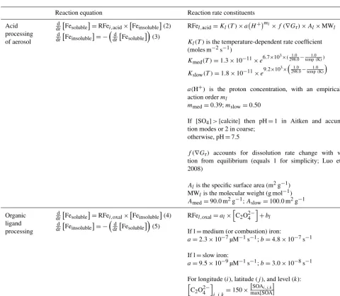
Once airborne, iron undergoes a series of physical and chem-ical processing steps within the atmosphere, each working to alter the soluble iron fraction (i.e. its solubility). The MIMI atmospheric iron dissolution scheme is presented in Table 5, with a full description reported previously by Scanza et al. (2018). Within each of the three iron-bearing aerosol size modes, six tracers of iron were advected within the model: medium-insoluble and medium-soluble mineral dust iron (containing both readily released and medium-reactive mineral dust iron; Scanza et al., 2018), slow-insoluble and slow-soluble mineral dust iron, and insoluble and soluble py-rogenic (sum of fires and anthropogenic combustion) iron, which was assumed to be medium-reactive (Scanza et al., 2018). Both proton- and organic-ligand-promoted iron dis-solution mechanisms were modelled. The proton-promoted dissolution scheme was dependent upon an estimated [H+], calculated from the ratio of sulfate to calcite, and the simu-lated temperature. Organic ligand dissolution was dependent upon the simulated secondary organic carbon concentration as oxalate (the main reactant) itself was not modelled. Both the sulfate and secondary organic carbon aerosol (Fig. S1 in the Supplement), which the iron processing requires, are fundamental components of aerosol models (e.g. Kanakidou et al., 2005; Mann et al., 2014). In CAM sulfate is mainly formed via the oxidation of SO2(aq)with a smaller contribu-tion from H2SO4condensation on aerosol, while secondary organic aerosol is formed via the partitioning of semi-volatile organic gases (Liu et al., 2012). Neither gas-to-particle pro-duction processes are structurally modified from the descrip-tion of CAM5 by Liu et al. (2012, 2016) by the incorpo-ration of MIMI. A structural model improvement was that MAM (CAM5) advected separate tracers for the interstitial and cloud-borne aerosol phases, so the proton- and organic-ligand-promoted dissolution reactions were applied to each aerosol phase, respectively.
Table 5.Summary of atmospheric processing reaction equations from Scanza et al. (2018). Herelrepresents either medium- or slow-reacting iron aerosol (combustion iron is modelled as medium). The pH calculation is updated to be calculated within each mode, and oxalate (C2O24−) concentrations are calculated based only on the secondary organic aerosol (SOA) concentrations.
Reaction equation Reaction rate constituents
Acid processing of aerosol
d dt
Fesoluble=RFei,acid×Feinsoluble(2) d
dt
Feinsoluble
= −
d dt
Fesoluble
(3)
RFel,acid=Kl(T )×a H+ml×f (∇Gr)×Al×MWl
Kl(T )is the temperature-dependent rate coefficient (moles m−2s−1)
Kmed(T )=1.3×10⁻¹¹×e
6.7×10³×( 1.0 298.0−
1.0 temp(K))
Kslow(T )=1.8×10⁻¹¹×e
9.2×103× 1.0 298.0−
1.0 temp(K)
a(H+) is the proton concentration, with an empirical re-action orderml
mmed=0.39;mslow=0.50
If [SO4]>[calcite] then pH=1 in Aitken and accumula-tion modes or 2 in coarse;
otherwise, pH=7.5
f (∇Gr) accounts for dissolution rate change with varia-tion from equilibrium (equals 1 for simplicity; Luo et al., 2008)
Alis the specific surface area (m2g−1) MWlis the molecular weight (g mol−1)
Amed=90.0 m2g−1;Aslow=100.0 m2g−1
Organic ligand processing
d dt
Fesoluble
=RFei,oxal×
Feinsoluble
(4) d
dt
Feinsoluble= −
d dt
Fesoluble
(5)
RFel,oxal=al× h
C2O24− i
+bl
If l=medium (or combustion) iron:
a=2.3×10⁻⁷µM−1s−1;b=4.8×10⁻⁷s−1
If l=slow iron:
a=9.5×10⁻⁹µM−1s−1;b=3.0×10⁻⁸s−1
For longitude (i), latitude (j), and level (k): h
C2O24−i
i,j,k=150×
SOAi,j,k max[SOA]
contained within it (Ingall et al., 2018; Longo et al., 2016; Meskhidze et al., 2003; Solmon et al., 2009), and mineral-ogy is a key factor determining the rate of dissolution at a given pH (Journet et al., 2008; Scanza et al., 2018). Mod-elled aerosol pH in MIMI was parameterized to depend only on the ratio of the calcium to sulfate aerosol concentration (Scanza et al., 2018). At each time step, if [SO4]>[calcite], then the aerosol was assumed to be acidic with a low pH, while if [SO4]<[calcite], then aerosol was assumed to be well buffered (Böke et al., 1999) and the pH=7.5. In MIMI, we updated the pH calculation from BAM-Fe in two ways: (1) in BAM-Fe, pH was calculated as the mean across all four size bins (0.1–10 µm), while in MIMI, pH was cal-culated separately for each interstitial aerosol size mode. (2) Aerosol measurements of pH have shown that
intersti-tial aerosol is likely to be more acidic than was assumed in BAM-Fe (Longo et al., 2016; Weber et al., 2016), even when taking into account declining sulfate levels (Weber et al., 2016); therefore, we have lowered the aerosol pH to 1 (from 2) in both the Aitken and accumulation modes wherein sulfate aerosol dominates. However, in the coarse mode, wherein dust dominates, we retained the lower pH bound-ary of 2. Furthermore, MAM aerosol was simulated as an in-ternally mixed aerosol; therefore, the SO4: Ca ratio included the mixing of these aerosol components within each mode. See Sect. 4.2 for a comparison of acid processing in MIMI with the literature and the previous model (BAM-Fe).
ligand reaction only proceeds within MIMI if the condition that cloud is present in the grid cell is first met. If cloud is present then only the iron aerosol which is associated with water undergoes organic ligand processing (i.e. the intersti-tial aerosol component remains unchanged). Any future de-velopment of MIMI within an aerosol model which does not advect a separate tracer for the cloud-borne phase of aerosol would therefore need to adjust the reaction to take account of this. An assumed oxalate concentration in MIMI was esti-mated based on the modelled organic carbon concentration and could not exceed a maximum concentration threshold of 15 µmol L−1 (Scanza et al., 2018). In BAM-Fe, oxalate was derived from the sum of both the primary and secondary organic carbon aerosol concentrations, while in MIMI this was updated to be dependent only upon the secondary or-ganic carbon source because oxalate is itself a product of the oxidation of volatile organic carbon gases (Myriokefalitakis et al., 2011). An additional term was added to the reaction mechanism to account for the small amount of organic ligand processing proceeding by species other than oxalate (Scanza et al., 2018). See Sect. 4.2 for a comparison of in-cloud or-ganic dissolution in MIMI with the literature and the previous model (BAM-Fe).
2.4.2 Computational costs
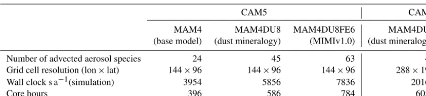
Earth system models are generally characterized by having a heavy computational burden in simulating atmospheric pro-cesses. The inclusion of MIMI requires eight dust mineral tracers (a net addition of seven) and six iron tracers. The total number of new aerosol tracers is 39 (13 in each of the three aerosol modes) if dust mineralogy is not already present or 18 new aerosol tracers if it is (e.g. NASA GISS model; Perlwitz et al., 2015a, b). The additional computational cost of MIMI within CESM-CAM5 is approximately a doubling of the re-quired core hours; around half of that is associated with dust mineralogy speciation and the other half with iron speciation and processing (Table 6). Note that additional computational tuning, or changes in configuration, could modify these com-putational change estimates. For example, with dust mineral-ogy (MAM4DU8) there is an approximate tenfold increase in required core hours due to model structural differences when transitioning from CAM5 to CAM6.
2.5 Observation and model iron calculations 2.5.1 Spatially aggregating limited observations The observations of total iron concentrations and the frac-tional solubility of iron used in this study are joint totals (1524 records) of those reported in Mahowald et al. (2009) and Myriokefalitakis et al. (2018). However, many of these observations represent averages of only one or a few days of iron and soluble iron measurements and can thus be diffi-cult to compare against annual, or longer, mean time periods
calculated within the model. Furthermore, building empirical distributions of iron properties from observations requires a larger sample size than currently available in many regions. We therefore tested how aggregating the observations spa-tially, sometimes termed “super-obbing”, altered our model evaluation. Our objective was to capture the small regional-scale properties of iron and not those at a point source; there-fore, we assume that the benefits gained by aggregating in this way, which include helping to produce a statistically use-ful number of observations, outweigh any potential biases. 2.5.2 Variations in model temporal averaging
The model was run at a 30 min time resolution. At each 30 min time step, soluble iron, total iron, and the ratio of soluble to total iron (iron solubility) were computed. The model output wasSi, (daily mean soluble iron concentration on dayi),Ti (daily mean total iron concentration on dayi), andRi (daily mean iron solubility on day i). Note that Ri is the daily mean of the calculated 30 min solubilities and hence is not equal toSi/Ti. We define online solubility as the average of ratios calculated as follows:
n
X
i=1 Ri
!
/n, (6)
wheren represents the total number of records over which the average was calculated. Online solubility is reported throughout this study. In Sect. 3.4, we then compare the av-erage of ratios to the ratio of avav-erages (defined as offline sol-ubility), calculated as follows:
n
P
i=1 Si
/n
n
P
i=1 Ti
/n
= S
T, (7)
whereSandT are the grid cell averages of soluble and to-tal iron concentrations, respectively, over the toto-tal time pe-riod considered in this study (2007 to 2011). While Eq. (7) is common within the literature, this methodology can produce larger variability in iron solubility across grid cells because it is based on both soluble and total iron annual mean con-centrations. In the online method, variability is reduced as extreme values in soluble and total iron concentrations gen-erally do not occur at the same time. We can define the oc-currence of extreme values, with respect to the time frame considered, by analysing a relativeZ-score metric calculated as follows:
ZFe,t=
Fet−Fet σFet or
ZFe,s=
Fes−Fes
σFes
Table 6.Simulation time (in seconds per simulated year) for the CESM-MAM4 model. The CAM5 base model, with the addition of dust mineralogy and with the addition of dust mineralogy and iron processing (i.e. MIMI v1.0), is shown. The cost of running the new higher-resolution CAM6 model with dust mineralogy is also shown for comparison. All CAM5 simulations were executed on 10 nodes with 36 cores per node for 2 years (2006–2007) with consistent output fields. CAM6 simulations are executed on 30 nodes with 36 cores per node.
CAM5 CAM6
MAM4 MAM4DU8 MAM4DU8FE6 MAM4DU8
(base model) (dust mineralogy) (MIMIv1.0) (dust mineralogy)
Number of advected aerosol species 24 45 63 46
Grid cell resolution (lon×lat) 144×96 144×96 144×96 288×192
Wall clock s a−1(simulation) 3954 5856 7836 20167
Core hours 396 586 784 6051
where Fe is either total (Fet) or soluble (Fes) iron. The rela-tive normalizedZscore can then be calculated as follows:
n
X
i=1
(zt,i−zs,i)/zt,i, (9)
whereZt,i andZs,iare theZscores of total and soluble iron concentrations, respectively, at each grid cell for each time stepi. TheZ-score metric provides a relative direction and distance of an instantaneous value with respect to its mean. The Z score is reported in multiples of the standard devia-tion (Eq. 8); therefore, a Z score of zero indicates that the data point value is identical to the mean value. To assess the relative difference in the variability at a given time be-tween the modelled total and soluble iron concentration and its mean, we calculated the difference in Z scores between total and soluble iron concentrations and normalized it using theZscore of total iron concentration (Eq. 9). Note that the
Z score of the soluble iron concentration could also be used to normalize the difference. This method allows for the ex-amination of how the occurrence of extreme concentration values in total and soluble iron influences the method of sol-ubility calculation (Eq. 6 vs. Eq. 7).
2.6 Iron ocean deposition source apportionment An ocean deposition source apportionment sub-study was designed to classify ocean deposition regions according to the dominant atmospheric soluble iron source, rather than ocean basins defined from a more traditional physical oceanographic viewpoint (e.g. Gregg et al., 2003). By incor-porating recent model estimates for dust and the importance of pyrogenic iron emissions (Luo et al., 2008; Matsui et al., 2018) the seven large-scale source regions defined in Ma-howald et al. (2008) were modified slightly to separate the major dust iron source regions from fire and anthropogenic combustion iron source regions. This resulted in a total of 10 iron emission source regions (Fig. 1; see also Table S1 for details).
Simulations in the source apportionment study used BAM-Fe, as described in Scanza et al. (2018), with slight modifica-tion. Briefly, anthropogenic combustion iron emissions were increased by a uniform factor of 5, and iron from fires fol-lowed the updated Fe : BC ratio (Table 4) and seasonal vari-ability in the fire BC emissions, all as per MIMI. Aerosols were externally mixed in BAM, and therefore altering the regional aerosol loading did not affect aerosol transport or deposition in the more significant way it could in MAM, in which aerosols are internally mixed. This information was then used in Sect. 4.3 to compare differences in the daily mean deposition of soluble iron between the BAM-Fe and MIMI models within each defined ocean region.
3 Modelled dust and iron aerosol concentrations compared to observations
In terms of Earth system modelling and the biogeochem-istry that connects the land–atmosphere–ocean components, we are ultimately motivated to improve the magnitude of the atmosphere-to-ocean iron deposition flux and its frac-tional solubility (from which the soluble iron flux can be de-rived). We compare the model results with a series of obser-vations and herein highlight some of the problems discovered when directly comparing with a sporadic (in both space and time) observation dataset, as is currently common practice (Myriokefalitakis et al., 2018).
3.1 Global dust comparisons
Comparison of dust AOD with regional dust AOD ob-servations (Fig. 2) from the AERONET observational datasets (Holben et al., 1998), as subsampled in Albani et al. (2014), shows good agreement globally (correlation:r2=
Figure 1.Major iron aerosol emission source regions.
of 1768 Tg dust a−1 in BAM (Scanza et al., 2018) because dust lifetime has proportionally decreased (Table S2), which affects coarse-mode dust aerosol (wherein 98 %–99 % of to-tal dust mass is emitted) more than fine-mode dust aerosol. Globally, both dust concentrations (correlation: r2=0.89) and deposition (correlation: r2=0.83) are simulated well compared to observations within MIMI. A higher correlation of modelled dust concentrations with observations is calcu-lated in the Northern Hemisphere (NH;r2=0.89) compared to the Southern Hemisphere (SH;r2=0.67), but the gradi-ent of the line of best fit is further from 1 : 1 (NH: 1.22 vs. SH: 1.07). Conversely, for dust deposition a lower correlation with observations is simulated in the NH (r2=0.75) com-pared to the SH (r2=0.60) but with a gradient of the line of best fit closer to 1 : 1 (NH: 1.07 vs. SH: 0.72). Overall, the results presented in this study suggest an improvement on previous dust modelling complications related to under-estimating dust deposition when tuned to dust concentration (Huneeus et al., 2011).
3.2 High-latitude dust and iron aerosol
Including the parametrization of Kok et al. (2014a) removes the requirement of a soil erodibility map (Table 1). In ad-dition, in previous versions of the model, high-latitude dust sources were zeroed because there were no observations at that time to support high-latitude sources of dust (Albani et al., 2014). However, more recent observations have sug-gested that high-latitude dust sources do exist (Bullard et al., 2016; Crusius et al., 2011; Tobo et al., 2019), often related to glacial processes (Bullard, 2017) with a higher fraction of bioavailable iron relative to lower-latitude dust sources (Shoenfelt et al., 2017). Thus, for the new version of the model we have allowed for the inclusion of high-latitude dust sources (Fig. 3). In general, aerosol dust and iron concentra-tions peak closest to the coastlines and during summer. Emis-sions of dust from>50◦N are∼1.3±0.2 % of the global dust total, which is half of the estimates derived from field
and satellite data at 2 %–3 % of the global total (Bullard, 2017; Bullard et al., 2016). However, the resulting magnitude and seasonality of dust concentrations have been shown in a recent study to be consistent with observed measurements from Svalbard (Tobo et al., 2019).
3.3 Global iron aerosol concentration and fractional solubility
There are several propositions explaining sources of soluble iron and the inverse relationship between total iron amount and iron solubility (Sholkovitz et al., 2012). While total iron mass concentrations are dominated by desert dust sources, soluble iron can be a product of mineral dust processed in the atmosphere or emitted from pyrogenic sources (Chuang et al., 2005; Guieu et al., 2005; Ito et al., 2019; Luo et al., 2008; Meskhidze et al., 2003; Schroth et al., 2009). Previ-ous studies have shown that either of these can explain the inverse relationship and that the spatial distribution of data is required to provide more information (Mahowald et al., 2018). Therefore, we explored how to best use the spatial data to compare with the model results. The 5-year (2007 to 2011) mean iron concentration from MIMI is compared to an extensive dataset of observations of total iron and its fractional solubility (Fig. 4). The model captures the global mean observational total iron concentration well; however, relatively low regional correlations (r2<0.4) occur in the south Indian (r2=0.0), South Atlantic (r2=0.34), North American (r2=0.35), and high-latitude (r2=0.06) ocean regions, suggesting that future model improvements can be focused here.
atmo-Figure 2.Dust aerosol optical depth, surface concentrations, and deposition in modal aerosol model and observations (Albani et al., 2014; Holben et al., 1998). Correlation (r2), gradient (m), and inter-cept (c) shown for global (G), Northern Hemisphere (N), and South-ern Hemisphere (S) regions.
spheric emission information, pyrogenic iron sources, and at-mospheric processing of iron, an estimate of 2 % solubility leads to underestimates of observed iron solubility in nearly all HNLC ocean regions (Fig. 4).
Aggregating observations onto a lower-resolution grid (sometimes termed super-obbing) compared with the model can help reduce the representation error when comparing
Figure 3. High-latitude (>60◦N) dust (sum of eight mineral species and four dust–iron species) and iron (sum of four dust–iron species) mass concentrations (µg m−3) at the surface model level.
with such limited observations (Schutgens et al., 2017). Fig. 5 uses an observational resolution one-third that of the model, and the model-to-observation comparison of the mean state is thus improved. Persistent observation-based features of the local environment become more obvious, while less frequent ones conversely diminish. At this obser-vational resolution, the low total iron concentrations in the North Atlantic∼30◦N, as seen in Fig. 4, are perhaps not a common feature, and the model much more precisely rep-resents the climatological state here than Fig. 4 might sug-gest. However, examining the North Pacific reveals that the model imprecisely represents the mean state here. Potential missing iron sources in remote regions, such as the North Pacific, include the following: (1) shipping emissions (Ito, 2013), which have a high soluble iron content from oil com-bustion (Schroth et al., 2009); (2) volcanic emissions, which provide a localized “fertilizer” to the surface ocean owing to the macronutrients and trace metal nutrients contained within them (Achterberg et al., 2013; Langmann et al., 2010; Rogan et al., 2016); and (3) low Asian and South American aerosol concentrations, either through underrepresenting combustion emission sources (Matsui et al., 2018) or in the transport and deposition of aerosol within these regions (Wu et al., 2018). These are discussed in more detail in Sect. 5.1 and 5.2.
Figure 4.Daily mean model total iron concentration and solubility from 2007 to 2011. Observations (circles) overlaid (at resolution of the model grid) as a mean from 1524 individual records in Mahowald et al. (2009) and in Myriokefalitakis et al. (2018). Also shown are scatter plots of the model mean and standard deviation compared to each available observation and identified by oceanic region. Correlation (r2), gradient (m), and intercept (c) for total iron with observations shown for each region.
Figure 5.Daily mean model total iron concentration and solubility from 2007 to 2011. Observations (circles) overlaid (at a resolution one-third of the model grid) as a mean from 1524 individual records in Mahowald et al. (2009) and in Myriokefalitakis et al. (2018).
1.3) values. However, the arithmetic means are not similar (model: 2.5, observation: 9.6) and while a high observation value of 155 % is likely to be an outlier and should be at most 100 %, it still informs us about what is possible, and simply discounting it (even at an adjusted 100 %) would re-quire strong justification. It is therefore advisable to instead alter the estimator of the average. Comparing model to ob-servation differences calculated using the median or geomet-ric mean reveals that they are similar in magnitude, as one would expect for log-normally distributed data (Fig. 6 in-sert). Although the median is robust with respect to outliers, the model results may not exhibit a uniform Gaussian distri-bution (Fig. 6 insert; solid compared to dashed lines), and of-ten the number of available observations is also low (Fig. 7), suggesting that its use also requires careful consideration. An equivalent methodology to the geometric mean in Fig. 7 would be to first log transform the data before calculating the arithmetic mean. Arguments pertaining to the appropri-ate methodology for comparing model results to temporally limited observations extend beyond the iron aerosol exami-nation in this study to all aerosol comparisons with limited observations.
3.4 Calculating iron solubility
aver-Figure 6.Histogram of observations (n=21) and daily model results (2007 to 2011) of iron solubility between 16 to 20◦N and 27 to 32◦W (one observation point and nine co-located model grid cells in Fig. 5). Mean (dashed lines), geometric mean (dot-dash lines), and median (full line) values shown the above respective dataset colour line. Note that the single observation value of 155 % is off the scale and placed as such with the value given above. Insert: log plot for the same data (solid lines) with projected log-normal distribution from the mean and standard deviation of the data (dashed lines).
ages) has when calculating iron solubility (Fig. 8). Through-out this study, the percent of iron solubility was calculated at each model time step (30 min) and then the daily mean output was analysed (online; Eq. 6) at an annual or 5-year mean time resolution. It is also acceptable to use the simulated soluble and total iron concentrations to generate the annual or 5-year mean iron solubility in a post-processing step (offline; Eq. 7). The resulting differences between methods are not insignifi-cant (Fig. 8); however, the offline method creates a distribu-tion in which low iron solubility is generally lower and the highest (>18 %) iron solubilities are generally higher. Over-all, the global annual mean iron solubility calculated online is one-third (34 %; NH=40 %, SH=29 %) higher than when calculated offline.
The average relativeZscore (Eqs. 8 and 9) is around zero for most model grid cells (Fig. 9), indicating that they mostly followed similar temporal and relative magnitude trends. However, even if the average relative Z scores are around zero and the ratio of relative standard deviations is around one, the ratio of online- to offline-calculated iron solubility is most likely>1. Temporal differences in the soluble and total iron concentration might therefore be controlling the overall solubility at each model grid cell. We also find that the ratio of online and offline solubility is>1 for most of the cases when the ratio of the relative standard deviations of soluble and total iron is<1 (Fig. S2), indicating that the differences in both methods of iron solubility calculation are sensitive to
the differences in the relative size of the tails of the distri-bution. That is, if soluble iron has narrower tails compared to total iron at any grid cell, it is highly likely that a higher solubility will be obtained in the online method compared to offline. The extreme ratio of the tails of soluble and total iron is only found in specific regions with the highest tem-poral variability in emissions and modelled solubilization of insoluble iron (Fig. S2).
Field measurements have generally suggested an inverse relationship between total and soluble iron concentrations (Myriokefalitakis et al., 2018). This means that high total iron concentrations are generally accompanied by low solu-ble iron concentrations and vice versa. By assuming that the field measurements faithfully represented the actual average values of soluble and total iron concentration at those loca-tions, we implicitly assume that all the measurements have a
Zscore of zero. In Fig. 9 we show that this is not the case with the modelled results, and the two variables can be rel-atively farther from their respective means even when aver-aged over the modelled time period.
Figure 7. Daily arithmetic mean, geometric mean, and median model solubility (2007 to 2011). Observations are overlaid (at res-olution one-third of the model grid) as the arithmetic mean, geo-metric mean, or median with respect to the model averaging. The number of observations is denoted by symbols: lowest confidence (one observation, diamond); intermediate confidence (two to four observations, triangle); highest confidence (five or more observa-tions, circle).
2014). It will also be important to consider differences in the solubility of iron induced by the choice of the order of op-erations as ocean biogeochemical models move away from using offline results from global climate or chemistry trans-port models to online results within Earth system models, which are designed to couple the two components at each time step. For short-term interactions between deposited iron and ocean biota, shorter-term averaging may be more impor-tant (e.g. Guieu et al., 2014), but for the long-term accumula-tion of iron that is (re)cycling in the oceans, the longer-term average may be more appropriate (Moore et al., 2013). One should be aware, however, that iron is readily removed from the ocean mixed layer, and thus the lifetime of iron may well be short enough for the online calculation to be more appro-priate much of the time (Guieu et al., 2014).
4 MIMI vs. BAM-Fe
In this section, we discuss how the new modal aerosol-mode version of MIMI compares to its predecessor bulk aerosol model version (BAM-Fe) throughout all three stages of the atmospheric iron life cycle.
4.1 Iron emission comparison
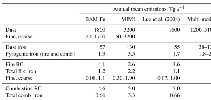
Globally averaged emissions of dust (3200 Tg a−1) and its iron component (126 Tg a−1) are within the current multi-model range (Table 7). The simulated annual mean iron in dust percentage is 4.1 %, with the highest percent occurring in the coarse mode at 6.5 % and the lowest percent occurring in the Aitken mode at 1.1 %. Accounting for dust mineralogy therefore increases the global mean iron percent by weight above the currently well-used global mean estimate of 3.5 % (e.g. Jickells et al., 2005; Shi et al., 2012).
Compared to BAM-Fe, MIMI dust emissions are∼80 % higher and the iron it contains is∼120 % higher (Table 7). Although both the BAM-Fe and MIMI models are globally tuned to a similar dust AOD (∼0.03) and based within the same host model (CESM), changing from a bulk aerosol scheme (e.g. Albani et al., 2014; Scanza et al., 2015) to a modal aerosol scheme reduces the aerosol lifetime signifi-cantly (Liu et al., 2012 and Table S2). The spatial distribu-tion of dust emissions is also different following the move to the Kok et al. (2014a, b) parameterization (Table 1), result-ing in the spatial distribution of dust AOD also beresult-ing altered (Fig. S3). Total pyrogenic iron emissions (sum of fires and anthropogenic combustion activity) in MIMI are higher than previous estimates by a factor of between 2 and 3 (Table 7), reflecting the growing evidence that they have been previ-ously underestimated (Conway et al., 2019; Ito et al., 2019; Matsui et al., 2018).
4.2 Iron atmospheric processing comparison
Figure 8.Mean solubility of iron when solubility is calculated at each 30 min model time step (“online”) and when it is calculated from the post-processing of daily mean soluble and total iron concentration (“offline”).
Table 7.Dust, fire, and anthropogenic combustion emissions of iron and relevant co-emitted aerosol emissions (to two significant figures). Multi-model emission range from the four global atmospheric iron models (including BAM-Fe) reported in Myriokefalitakis et al. (2018). Fine (sum of Aitken and accumulation modes) and coarse (coarse mode) mass emissions also given for dust, fire iron, and combustion iron.
Annual mean emissions; Tg a−1
BAM-Fe MIMI Luo et al. (2008) Multi-model
Dust 1800 3200 1600 1200–5100
Fine, coarse 20, 1700 50, 3200
Dust iron 57 130 55 38–130
Pyrogenic iron (fire and comb.) 1.9 5.5 1.7 1.8–2.7
Fire BC 4.1 2.6 3.6
Total fire iron 1.2 2.2 1.1
Fine, coarse 0.08, 1.1 0.30, 1.90 0.07, 1.00
Combustion BC 4.6 5.0 5.0
Total comb. iron 0.66 3.3 0.66
Fine, coarse 0.10, 0.56 0.50, 2.80 0.10, 0.56
Comparison of Fig. 10 to modelled pH estimates by Myriokefalitakis et al. (2015) shows generally good agree-ment in the NH, but in the SH MIMI simulates less acidic coarse-mode aerosol over continental regions and more acidic aerosol over marine regions. As iron models are un-able to capture the high observed iron solubility (>10 %) over SH marine regions (Myriokefalitakis et al., 2018) and in the absence of remote pH aerosol observations, we sug-gest that our basic parameterization captures an aerosol pH which is suitable for use in Earth system models
Model physics, and hence simulated cloud cover, are sig-nificantly different between CAM4 and CAM5. Figure 11a shows the relative model difference in the oxalate distribution between MIMI, which also includes an increase in the tuning factor by an order of magnitude (from 15 to 150; Table 5), and BAM-Fe by normalizing by the simulated cloud fraction in each model. The effect of oxalate on iron dissolution is therefore larger in MIMI over extratropical ocean regions, where iron models underrepresent solubility
(Myriokefali-takis et al., 2018), and land regions which are dense in trop-ical vegetation or industry (both centres of large aerosol pre-cursor gas emissions). Compared to observations (Myrioke-falitakis et al., 2011; Table S3) modelled oxalate concentra-tions are well represented at high observed concentraconcentra-tions but are biased low when observed concentrations are low (Fig. 11b). The low model bias is stronger within remote ob-servational regions (marine vs. urban observation sites), sug-gesting that the removal of secondary organic aerosol may be too strong within the model and/or that there is a missing marine aerosol precursor gas emission source (Facchini et al., 2008; O’Dowd and de Leeuw, 2007) in this model which sig-nificantly lowers simulated secondary organic aerosol, and thus oxalate, concentrations.
Figure 9.Relationship of online- to offline-derived iron solubility to the relativeZscore for total (ZFet) and soluble (ZFes) iron and the relative standard deviation (σFe/Fe) at each grid cell for the year 2007.
Figure 10. Surface-level annual mean interstitial aerosol pH. If [SO4]>[calcite] then pH=1 in Aitken and accumulation modes or 2 in coarse; otherwise, pH=7.5 (Table 5).
most regions of the world. A notable difference exists in the North Pacific region, where the soluble iron source in MIMI is lower than all other iron models, similar to total iron concentrations when compared to observations (Figs. 4 and 5). Future development of MIMI should thus be focused on the North Pacific, including the addition of shipping sol-uble iron emissions, which are relatively concentrated in this region (Ito, 2013). An improvement for MIMI can be seen over the Atlantic region directly downwind of Saharan solu-ble iron sources. In general, iron models are overrepresenting iron solubility close to dust sources compared to observa-tions (Myriokefalitakis et al., 2018), and in order for BAM-Fe to reach better agreement with observed iron solubility in
this region dust emissions of soluble iron had to be scaled downwards (Conway et al., 2019). We suggest that this im-provement is linked to the improved modal representation of aerosol pH in MIMI (Fig. 10).
4.3 Iron ocean deposition flux comparison
Similar to the previous study by Scanza et al. (2018), we re-port the amount of total and soluble iron deposited in each of the major ocean basins (Table 8) as defined by Gregg et al. (2003). We find that in MIMI the amount of total iron deposited to all ocean basins is approximately double that estimated in BAM-Fe (26 vs. 12 Tg Fe a−1, respectively), while soluble iron deposition is similar (∼0.5 Tg Fe a−1in both models). The larger mineral dust emission flux in MIMI (3200 Tg dust a−1 compared to BAM-Fe dust emissions of 1800 Tg dust a−1) is driving most of the increases in total iron deposition because it is the primary iron source (Ta-ble 7). In general, the magnitude of solu(Ta-ble iron deposition to the oceans is more evenly distributed across hemispheres in MIMI owing to a major reduction (approximately one-half) in the equatorial north–central Atlantic basin deposi-tion flux and increases to SH ocean deposideposi-tion fluxes of a factor of 2 to 4. In MAM4 dust is treated as internally mixed aerosol with sea salt, leading to higher rates of wet deposi-tion than when dust is externally mixed aerosol (Liu et al., 2012) as it is in CAM4. The internally mixed treatment of dust aerosol in MAM4 is thus an important factor leading to the lower simulated dust lifetime when compared to BAM-Fe (Table S2). Over the north–central Atlantic region, the com-bination of a lower soluble iron source (Fig. 12 compared to Fig. S4b by Myriokefalitakis et al., 2018), dust atmospheric lifetime (Table S2), lower aerosol pH (Fig. 10), and lower relative organic ligand processing (Fig. 11) will all work to-wards reducing the magnitude of atmospheric soluble iron deposition flux in MAM4 compared to BAM-Fe. There are significant increases in anthropogenic combustion iron de-position in all equatorial and NH ocean basins driven by the fivefold increase in combustion emissions implemented in MIMI. The percent contribution from pyrogenic iron to total iron deposition between MIMI and BAM-Fe is, how-ever, more similar for all northern and equatorial oceanic regions than southern oceanic regions. Beyond the correc-tion to anthropogenic combuscorrec-tion emissions, which are NH dominated, this could be due to differences in the emissions of both dust and fire aerosol, structural differences between models relating to the aerosol size and composition, which alters aerosol deposition rates, or a lower soluble iron source (Fig. 12); it is most likely to be a combination of all three.
Figure 11. (a)Relative difference in organic ligand reaction on in-cloud iron aerosol dissolution between MIMI and BAM-Fe. Due to significant differences in simulated cloud cover between CAM4 and CAM5 oxalate concentrations [OXL] are multiplied by the model-simulated cloud fraction in this figure. (b)Surface-level oxalate (OXL) concentration in the model and observations. Model values are monthly mean (2007–2011) and annual standard deviation. Observation values are from Table S3 in Myriokefalitakis et al. (2011) and reported with uncertainty where given.
Table 8.Global and regional ocean basin deposition (Gg a−1) of total and soluble iron in BAM-Fe (Scanza et al., 2018) and MIMI (this study). Deposition was multiplied by the ocean fraction of model grid cells and is reported at two significant figures. The percent contribution from pyrogenic (sum of fires and anthropogenic combustion) iron sources to deposition is also given. Ocean basins are those defined by Gregg et al. (2003) and previously used by Scanza et al. (2018).
Dust and comb. deposition; Gg a−1 Percent iron from pyrogenic sources; %
Total iron Soluble iron Total iron Soluble iron
BAM-Fe MIMI BAM-Fe MIMI BAM-Fe MIMI BAM-Fe MIMI
Global 12 000 26 000 500 530 3.3 5.0 7.6 23
N. Atlantic 1800 5300 46 86 1.9 2.9 4.8 11
N. Pacific 730 1200 35 36 10 19 15 43
NC. Atlantic 2900 5700 92 89 0.30 0.52 0.9 3.7
NC. Pacific 230 300 16 12 7.9 24 10 56
N. Indian 2700 7000 62 101 1.2 2.1 3.9 10
Eq. Atlantic 2600 2600 190 95 2.8 9.9 5.5 34
Eq. Pacific 59 91 6.2 6.7 21 37 25 68
Eq. Indian 830 1200 35 39 5.9 12 11 38
S. Atlantic 65 790 4.1 16 30 4.8 50 25
S. Pacific 21 250 1.4 6.4 41 7.8 50 30
S. Indian 42 200 3.0 6.9 51 16 58 46
Antarctic 270 1300 12 37 20 12 48 44
ocean regions (Fig. 13). In general, vertically distributing fire emissions results in small increases in soluble iron deposition (between 0 % and 20 %) in SH ocean regions and a larger increase (between 20 % and 40 %) in NH oceans, with con-verse lower land deposition close to the major regions of fire activity. The exception is in the sub-Arctic North Pacific, an HNLC region, where iron deposition from fires significantly increased until it was more than double that when surface fire emissions are used.
The dry deposition flux is sensitive to aerosol properties, surface roughness, and modelled turbulence. Although in-creasing the vertical resolution has been shown to increase
surface PM10 concentration (Menut et al., 2013) and better simulate the dust vertical profile (Teixeira et al., 2016), it is not yet clear if this would correspondingly increase the dry deposition flux.
Source region comparison
exam-Figure 12.Annual mean dust and pyrogenic (sum of fires and an-thropogenic combustion) soluble iron source (i.e. sum of emissions and atmospheric processing).
Figure 13. The ratio of soluble iron deposition from fires when emissions are emitted with a vertical distribution to fires when emis-sions are only at the surface (i.e. vertical/surface). Single year (2007) comparison only.
ined, and from this the boundaries of each region in Fig. 14 were delineated. The resulting eight ocean iron deposition regions are split equally into four in the NH and four in the SH. Note, however, that the NH–SH divide sits at 15◦S and not the Equator, which is due to transport differences in each hemisphere and the position of the Intertropical Convergence Zone. Of the four regions that can be defined as major dust deposition receptors (Fig. 14; bottom panel bar chart), the north Indian Ocean (no. 1), North Atlantic and central Pacific (no. 4), and South American dust (no. 7) regions have a sin-gle dominant source each, while the North Pacific (no. 3) re-gion is more variable. These dust-dominated iron deposition regions are similarly reproduced by other global iron mod-els (Ito et al., 2019; Myriokefalitakis et al., 2018). The re-gions of the mixed Southern Hemisphere oceans (no. 5) and Australian and South Pacific (no. 6) receive similar amounts of mineral dust and pyrogenic iron, suggesting that the iron sources are spatially closer and thus share much more similar transport pathways than the South East Asian ocean (no. 2) and South American pyrogenic (no. 8) regions, which have a much more distinct pyrogenic iron source signal. Deposition
Figure 14. (a) Eight soluble iron ocean deposition regions de-fined by dominant source region apportionment. Region 1: north Indian Ocean (NIND). Region 2: South East Asian ocean (SEAS). Region 3: North Pacific (NPAC). Region 4: North Atlantic and central Pacific (NACP). Region 5: Southern Hemisphere oceans (SHOC). Region 6: Australian and southern Pacific (AUSP). Re-gion 7: South American dust (SADU). ReRe-gion 8: South American pyrogenic (SAPY).(b)Contribution of each emission source region (Fig. 1) to the total iron deposition across the region. Contributions of dust and pyrogenic (sum of fires and anthropogenic combustion) iron from the source region are also shown. Regions contributing
<5 % are filtered out.
regions are more clearly defined when using this methodol-ogy compared to those from a more traditional classification of ocean basins based on physio-geographical oceanography (Fig. S4). This information can be used to assess which ocean regions are most likely to be affected by anthropogenic per-turbations to the magnitude of iron sources within different regions, whether through land use, land cover change, or in-dustrialization.
tempo-rally static in both model frameworks and therefore do not affect the variability in this study as much as fires and min-eral dust but will in the future if this is changed to repre-sent a seasonal emission cycle. We can see that each of the dust and fire updates in MIMI have a large impact by com-paring the Patagonian dust-dominated South American dust (SADU) region and the fire-dominated South American py-rogenic (SAPY) region. Most of the dust deposited (30 % to 90 %) in the ocean occurs during large dust events that are on just 5 % of the days (Mahowald et al., 2009), result-ing in large differences between median and mean deposition amounts in all regions, as seen in Fig. 15. It is important to note that the mean is always above the interquartile range, further supporting our previous arguments pertaining to the modelled mean not being an ideal estimate of the average as it does not represent the log-normal distribution of aerosol. Comparing the mean-to-median ratio suggests that extreme dust events are also more pronounced in MIMI (CAM5) than in BAM-Fe (CAM4).
5 Future directions
The purpose of model-to-observation comparisons is to iden-tify situations (regions, times, model settings, or combina-tions thereof) in which the model output is inconsistent with observed realities, with the goal being to further refine the model in the future. Each individual observation represents a snapshot of the atmospheric state at a specific point in space and time, and when an observation falls outside the distri-bution of model output values from the same location and time, we can view this as evidence of a model misspecifica-tion. For the example of iron modelling, constraining current model–observation discrepancies would benefit from further exploring the model sensitivity of simulated iron and its sol-ubility to uncertainties in five major parameter sets: dust iron emissions, pyrogenic iron emissions, atmospheric iron dis-solution chemistry, dry deposition rates, and wet deposition rates. In general, improving the modelled representation of secondary organic aerosol (including oxalate) and aerosol pH, particularly for remote regions, is an important task for aerosol modelling and one which would have co-benefits for iron aerosol modelling. Comparisons of the soluble fraction of other aerosol species with observations could also be used to guide model development.
Here we discuss some of the model parameters which are likely important for improving modelled iron emissions and deposition in MIMI, and thus iron process models in general, in the future.
5.1 Improving iron aerosol emissions
Downwind of significant mineral dust sources iron mod-els generally overestimate the observed amount of total iron (Myriokefalitakis et al., 2018), and soluble iron comparisons
Figure 15.Violin plots of 5 years of log10daily soluble iron deposi-tion (µg m−2d−1) within each grid cell for the eight ocean regions defined in Fig. 14. Only grid cells in which ocean fraction>0.5 are included in the analysis. Violin colour matches Fig. 1 region colour: north Indian Ocean (NIND); South East Asian ocean (SEAS); North Pacific (NPAC); North Atlantic and central Pacific (NACP); South-ern Hemisphere oceans (SHOC); Australian and southSouth-ern Pacific (AUSP); South American dust (SADU); South American pyrogenic (SAPY). Violin outline colours: blue lines: BAM results, orange lines: MAM results. Black cross: log10mean daily soluble iron de-position. Median, mean, and ratio (mean/median) values for all 5 years of daily deposition amounts across each basin are also given.
are highly sensitive to the assumed initial solubility of min-eral dust iron at emission (Conway et al., 2019). Conversely, in remote ocean regions, improving the representation of combustion emissions has been shown to be a necessary step towards more accurate representations of observed high iron solubilities at low iron concentrations (Ito et al., 2019). 5.1.1 Mineral dust iron aerosol emissions