Scheduling of Workflow Applications based on Width of the Graph in Grids (SWAWGG)

S

S

C

C

H

H

E

E

D

D

U

U

L

L

I

I

N

N

G

G

O

O

F

F

W

W

O

O

R

R

K

K

F

F

L

L

O

O

W

W

A

A

P

P

P

P

L

L

I

I

C

C

A

A

T

T

I

I

O

O

N

N

S

S

B

B

A

A

S

S

E

E

D

D

O

O

N

N

W

WI

ID

DT

T

H

H

O

O

F

F

T

T

HE

H

E

GR

G

R

AP

A

P

H

H

IN

I

N

G

GR

R

ID

I

DS

S

(

(S

S

WA

W

A

WG

W

GG

G

)

)

S

Sr

ri

i

ka

k

al

l

a

a

K

Ke

e

s

s

he

h

et

t

ti

t

i

,

,

R

Ra

am

ma

ac

c

ha

h

an

nd

dr

r

am

a

m

S

Si

ir

r

an

a

nd

da

as

s

1

TutorVista Global Pvt. Ltd., Department of Mathematics

2

Osmania University, Computer Science Department

ABSTRACT: Grid applications require allocation of distributed resources to a number of heterogeneous tasks. Effective Scheduling is a major concern of performance driven grid applications. A good allocation technique is nothing but efficient execution. Basically there are two different types of resource allocation algorithms.

1)Task based algorithms allocate resources to tasks using a Greedy approach.

2)Workflow based algorithms search for an efficient allocation for the entire workflow.

The workflow based approaches are better for data – intensive applications. In this paper, we are going to present a workflow - based technique that determines efficient mapping of tasks by calculating the task to be scheduled on to the available list of resources using the workflow task graph. Using simulation, we have implemented a workflow – based approach that uses a directed acyclic graph of workflow – based tasks. This Algorithm uses Breadth first traversal of the graph to schedule the tasks. Our results demonstrate that the width based scheduling of workflows can generate better allocation in grid where resource availability changes frequently.

KEYWORDS: Grid workflow, workflow scheduling, inter dependent tasks, Directed acyclic graph, distributed resources, ascending order allocation, descending order allocation , unordered allocation, level of the graph, parent node

1. INTRODUCTION

Grids have emerged as global cyber-infrastructure for the future-generation of e-business and e-Science applications, by integrating large-scale, heterogene ous, distributed resources. Many of the applications executed on grids are workflows. A workflow management system defines, executes and manages workflows on computing resources. A workflow is a set of linked inter dependent tasks. A workflow management system is responsible to define, manage and execute workflow applications on grid resources. A workflow management system may use a specific scheduling strategy for allocating the tasks in a workflow to suitable grid resources in order to meet the user requirements.Some workflow scheduling strategies have been proposed in literature. Jia Yu et al [YBR08] discussed existing workflow scheduling algorithms developed and

deployed by various grid projects. Jia Yu et al [YB06a] developed a genetic algorithm for opt imized scheduling. Jim Blythe et al [B+05] investigated that if underlying execution environment changes, the allocation may be redone. In this the execution time is high. Mustafizur Rahman et al [RVB07] developed a DCP-G (Dynamic Critical path for grids) algorithm this is designed for mapping tasks on to homogenous processors. These are some of the observations that bring new challenges in designing algorithm for workflow applications on grids. Scheduling of workflow applications based on width of the gra ph in grids (SWAWGG) addresses issues mentioned above.

The rest of the paper is organized as follows.

In section II we describe related work. Section III describes the SWAWGG. Section IV explains the process with an example. In section V we describe the SWAWGG algorithm. In section VI we discuss the complexities of the algorithms. Simulation environment and results are discussed in section VII. Finally, we conclude the paper in section VIII.

2. RELATED WORK

Review of literature reveals that grid envir onments are more failure prone as the resources may come and go at any time. Most of the time we get data intensive applications to be scheduled on grid. We use workflow – based algorithm for scheduling this type of tasks.

QoS requirements specified by the user and map workflows on available resources such that the execution of workflow can be completed to meet the QoS constraints specified by the user. Most QoS constraint based workflow scheduling is based on either cost or time constraints. SWAWGG algorithm is implemented using ascending order allocation, descending order allocation and unordered allocation depending on the prior constraints of cost and time which are specified by the user. For example when the constraint is cost it uses ascending order allocation and when the constraint is time it uses descending order allocation.In this algorithm we use the following terminology

Ascending order allocation: The resources are sorted in ascending order and allocated in the same order.

Descending order allocation: The resources are sorted in descending order and allocated in the same order.

Unordered allocation: In this the resources are not ordered, as and when the resource is available it is allocated to the gridlet that is waiting for the resource.

The main objectives of SWAWGG technique are i. Improves user benefit by completing the job

submitted by the user within the deadline. ii. Improves owner benefits by increasing the

resource utilization rate.

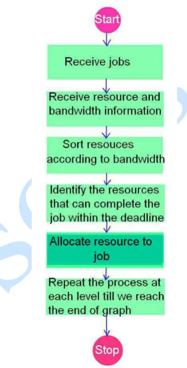
3. SCHEDULING ACTIVITY OF WORKFLO W APPLICATIONS BASED ON WIDTH OF THE GRAPH IN GRIDS (SWAWGG)

The grids are heterogeneous and dynamic environments consisting of network, storage and computing resources. The resources are sorted based on bandwidth. For a task graph the start time of each task is denoted as ST. This algorithm is des igned for scheduling all the tasks in a task graph with arbitrary communication and computation times to a set of grid resources. The terms gridlet, task and job are used interchangeably.For mapping a task on the resource, all avilable resources are considered and the time needed to complete the task on each resource is computed. The time is computed by using T=JOB_MI/RESOURCE_ MIPS.

Where T is the time needed to finish the gridlet. JOB_MI is the number of million instructions in the gridlet that is the required processing power and RESOURCE_MIPS is the Million instructions per second is the processing capacity of the resource. The resources that can complete the task within the deadline are identified and the task is assigned to the first resource that completes the job within deadline. When a task is mapped onto a resource the start time of each of the child node is calculated. The condition

for Scheduling a task from a task graph is we can schedule a task only when its parent task is completed execution. We follow the same procedure for scheduling next level nodes. That is our scheduling approach works based on width of the graph. Once we reach the end of the task graph the Algorithm stops.

Figure 1: Activity diagram for SWAWGG approach

Calculation of Start Time of each node in SWAWGG T = JOB_MI/ RESOURCE_MIPS

For each task Ti ST (Ti) = CT+T of PT

Where T is the Time in seconds required to finish the job.

ST (Ti) is the Start time of task Ti ST (Ti) = CT if Ti is the root Task CT is the Current Time

and PT is the Parent Task.

JOB_MI is the number of million instructions in the task.

available list of resources by traversing the task graph in breadth first manner and the task to be assigned has no unmapped parent tasks.

If the parent task is not completed its execution resource is free then the next task (T) whose parent completed execution is assigned to the resource and missed tasks of Breadth First Manner are kept in a Queue. Whenever a task is finished Queue is searched for the entry of its children.

Once the Parent task of missed tasks completes execution the tasks which are on the Queue are scheduled first then again it follows breadth first manner if there are any unmapped tasks.

Resource selection: After identifying the task to be scheduled, we need to se lect an appropriate resource for that task. The resources are sorted based on bandwidth in descending order. All the resources that can complete the task within the deadline are identified and the task is assigned to the first resource that completes the job within deadline. We call this allocation approach as descending order allocation. We use this approach because

If we use the descending order allocation approach the job is going to be finished much faster than the deadline.

This algorithm is also implemented by using unordered and ascending order allocation methods. Unordered allocation and ascending order allocation methods have the following advantages.

1) If we use descending order allocation, user has to pay more cost as the bandwidth of the resource is more. Since the job is done within the deadline usually end users prefer to get their job finished at lower cost.

2) If we select the descending order allocation approach next job may require a resource with higher than the available one, this causes the job to wait for execution and as a result all the child tasks are also delayed. This approach charges more from the user and there is no guarantee that it is completed much faster than the ascending order allocation.

Depending on the importance of execution time, Cost and resource utilization rate we can choose any one of the approaches among ascending order allocation, unordered allocation and descending order allocation.

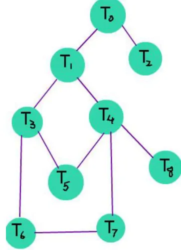
4. SWAWGG EXAMPLE

Figure 2a shows the workflow application. Figure 2 demonstrates mapping of tasks in a sample workflow with step by step explanation. The sample workflow consists of tasks T0, T1, T2, T3, T4, T5, T6, T7 and T8 with different data transfer and execution requirements. The task length and output size of each task are measured in million instructions and Kilo bytes respectively. These tasks are mapped onto four grid resources R1, R2, R3 and R4. We explain an

example using the descending order allocation of resources.

Figure 2a: Sample workflow of an application

In SWAWGG approach the external deadline that is the deadline by which workflow is to be completed is provided by the user. By using the External deadline internal deadlines for each of the task is generated depending on the length of workflow, length of each of the sub tasks and External deadline. After generating internal deadlines, resources that can complete the task with in limit are identified then using descending order allocation method resources are allocated to the subtask / gridlet. While traversing the graph of given workflow we use Breadth first Traversal.

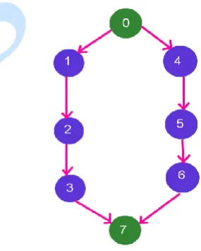
Figure 2b shows the Breadth first traversal of the graph of Figure 2a, External deadline given for the entire workflow and Total size of the workflow.

Figure 2b: Breadth First Search, length and deadline of the of graph 2a (Sample workflow)

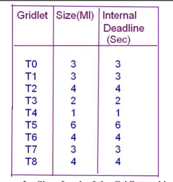
Figure 2c: Size of each of the Gridlet and internal deadline of each gridlet shown in graph 2a

The following are the available list of resources with their bandwidth that is processing power of resource shown in figure 2d.

Figure 2d: List of available resources and their bandwidth

As discussed earlier, the root task is scheduled first and the condition is until the parent task is completed the child task cannot be scheduled. The child task at each level is selected by following Breadth First Search (BFS) Traversal.

Figure 3: Resource allocation to gridlet and the Queue entries

As shown in figure 3 After T8 Breadth First Traversal gives us T7 but, unless its parent T6 is completed we cannot allocate resource to T7. Therefore T7 is stored in the Queue as shown above; T5 is not allocated until T3 finishes execution and T6 also dependent on T3. Once the current task finishes its execution a lookup operation to Queue is performed to search for the task whose parent completed execution just now. If there are any tasks waiting they will be scheduled next. The process continues in this way till all the tasks/ gridlets of the workflow are completed.

5. SWAWGG ALGORITHM

Figure 4 demonstrates the Algorithm for Scheduling of workflow applications based on width of the graph in grids.

Figure 4 demonstrates that the job to be mapped is found using Breadth First Search Algorithm of a graph.

If the job is the root job then it is mapped with the available resource.

If the job is not a root node and the status of its parent job is completed then the job is allocated with the next available resource.

Otherwise

If the parent job is not completed then the job will be waiting in the Queue and the next job t o be scheduled is the one whose parent completed the execution. All other jobs are stored in the Queue.

Once the Parent job is completed the waiting entries in the Queue are mapped first.

6. DISCUSSION

From our work it is evident that the Genetic algorithm is obtained by combining current best solutions and exploiting new search region over generations. The Genetic Algorithm is a Meta-heuristic best-effort workflow Scheduling Algorithm. DCP-G and SWAWGG are heuristic based best-effort workflow scheduling algorithms. DCP -G operates in batch mode ranking tasks based on critical path and re-ranking adjacent independent tasks is done throughout the algorithm. Complexity of DCP -G algorithm is O (v^2m+vgm) where v is the number of tasks in the workflow, m is the number of resources and g is the number of tasks in a group of tasks for the batch mode scheduling.

The complexity of SWAWGG algorithm is O (v(1+gm+logv)+e) where v is the number of vertices e is the number of edges is the number of resources available in the graph and g is the number of tasks in a group of tasks for the batch mode scheduling. SWAWGG algorithm is based on BFS approach, we use linear search for searching the Queue entries. Since the space is not a constraint with the present day computers and the solution can be found with the fewest arcs SWAWGG is a best approach when compared to DCP-G and GA.

Simulation results shown in the next section are based on SWAWGG using descending order allocation. We can see that as the resources in SWAWGG approach are already sorted and the entire graph is to be scheduled, SWAWGG algorithm gives good throughput. In case of a parallel workflow through put is much better than DCP-G because of ranking of nodes, finding the critical path and then re ranking nodes is the overhead in DCP-G. Throughput is almost same in case of a fork and join workflow that is number of jobs completed in the given time is same for the example we discussed. When it is tested with an arbitrary work flow it gives more throughput than the DCP-G Algorithm because we are using sorted list of resources and BFS. Instead of adjusting the graph every time SWAWGG uses a Queue where the gridlets which are waiting for their parents to be completed are stored. The complexity of SWAWGG is less when compared to DCP-G and GA. Simulation results shown in the next section give good results when compared to DCP-G and GA.

7. SIMULATION ENVIRONMENT AND RESULTS

The Algorithms for comparison DCP-G (Dynamic Critical path for grids) and GA (genetic algorithm) are implemented on a machine based on Pentium 1.6GHz with 120GB HDD and RAM of 1GB on Microsoft Windows XP. This experiment is carried

out on a simulated grid environment provided by GridSim.

The Simulation environment consists of resources. There are 4 resources having different processing capabilities in terms of Millions of Instructions per Second (MIPS). Further it is assumed that there are 8 gridlets.

SWAWGG is compared with DCP-G and GA the results are recorded on graphs.

The workflow generator can generate different workflows. The input parameters used for creating workflow are explained below.

Number of gridlets: Workflow consists of n number of gridlets.

Width of the workflow: Width of the workflow is the maximum number of nodes in a level.

The workflow generator can generate three types of workflows. They are explained below.

Parallel wo rkflow: In parallel workflow a set of gridlets make a chain with an entry and an exit gridlet. There can be several such chains in a workflow. Here one gridlet is dependent on only one gridlet, but the gridlets at the head of the chains are dependant on entry gridlet and the exit gridlet is dependent on the gridlets at the back of chains. A sample of parallel workflow is shown below

Figure 5a: Parallel workflow

Fork out and join in work flow: In this workflow forks of gridlets are created and then joined. That is it has one entry gridlet and one exit gridlet. A sample of fork out and join in workflow is shown below in figure 5.b.

Figure 5b: Fork out and join in workflow

Figure 5c: Arbitrary workflow

We evaluate the scheduling decisions on the basis of number of gridlets completed in the given amount of time. The resources that can complete the execution within the deadline are identified and then they are sorted in descending order if the prior constraint is time, when the prior constraint is cost the resources are sorted in descending order. The algorithm can also be executed using unordered allocation.

The following are the graphs drawn for comparison. figure 5d, figure 5e and figure 5f are the graphs drawn using descending order allocation.

Figure 5d:Parallel workflow

Figure 5d shows the graph between number of gridlets in the workflow and time taken by the workflow in case of a parallel workflow. From the figure we can see that SWAWGG is taking less time when compared to DCP-G and GA.

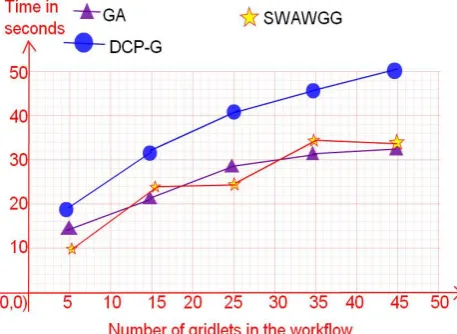
Figure 5e: Fork out and join in workflow

The number of gridlets in the workflow and their execution time for a fork out and join in workflow is plotted in the graph as shown in Figure 5e. The output of GA is not predictable because GA is obtained by combining current best solutions and exploiting new search region over generations. It can be observed that as the number of gridlets is increased there is increase in the execution time and by using SWAWGG is giving almost equal time when compared to GA and SWAWGG shows better results when compared to DCP-G.

Figure 5f: arbitrary workflow

search region over generations. These results demonstrate that SWAWGG algorithm gives better performance results when compared to DCP-G algorithm and genetic algorithm.

The SWAWGG Algorithm is tested using descending order allocation, unordered allocation and ascending order allocation methods. Resource utilization rate for each of the methods is shown in the following graph that is figure 5g.

The band width of the four resources considered for executing the workflow is given below.

R1 – 9.7 MIPS R2 – 4 MIPS R3 – 3 MIPS R4 – 1 MIPS

MIPS is the number of million instructions per second which is nothing but the resource processing capacity.

Figure 5g: resources and their utilization rate

According to the graph shown in figure 5g R1 (resource 1) is utilized more frequently when descending order allocation is used. R4 (Resource 4) is utilized more frequently when ascending order allocation is used. The green bars show the resource utilization rate using unordered allocation, in this allocation method the resources are not sorted and the available resource is assigned to the gridlet that is waiting for the resource irrespective of resource processing power and size of the gridlet.

Although the three allocation methods complete execution within the deadline given ascending order allocation is good when cost constraint is given, descending order allocation is good when time is the major constraint and when cost and time both are the constraints given we use unordered allocation in which resources are not sorted.

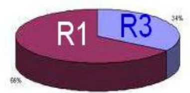
The following is a pie-chart demonstrates frequency of resource utilization for the example shown in figure 2a using descending order allocation.

Figure 5h: Resources R1 , R3 and their utilization rate

The resources with higher processing power are allocated each time when descending order allocation is used. Figure 5h shows the resource utilization of R1 (resource 1) and R3 (resource 3) for the sample workflow shown in figure 2a. The resource processing powers are shown in figure 2d. Resource 1 that is R1’s processing power is more therefore its utilization rate is higher than other resources. From the graph it can be observed that resource utilization rate of R1 is 66% and the next higher processing power resource is R3 whose resource utilization rate is 34%.

8. CONCLUSIONS

approach, ascending order allocation approach and unordered allocation approach.

Ascending order allocation approach improves user benefit by providing less cost. Descending order allocation approach improves user benefit by completing the workflow at a lesser time and unordered allocation approach improves resource owner benefit by minimizing the wastage of resources. Scheduling of workflow a pplications based on width of the graph in grid (SWAWGG) is a better approach for scheduling the workflow.

REFERENCES

[B+05] Jim Blythe, Sonal Jain, Ewa Deelman, Ken Kennedy, Anirban Mandal – Task scheduling strategies for workflow based

applications in grids IEEE International

Symposium on Cluster Computing and Grid (CCGrid), 2005.

[RVB07] Mustafizur Rahman, Srikumar

Venugopal, Rajkumar Buyya - A

dynamic critical path algorithm for

scheduling scientific workflow

applications on global grids, e-Science

and Grid Computing, IEEE International Conference 2007

[YB06] Jia Yu, Rajk umar Buyya - A Budget Constrained Scheduling of Workflow Applications on Utility Grids using

Genetic Algorithms, Workshop on

Workflows in Support of Large-Scale Science, Proceedings of the 15th IEEE International Symposium on High Performance Distributed Computing (HPDC), 2006.

[YB06b] Jia Yu, Rajkumar Buyya –Scheduling scientific workflow applications with deadline and budget constraints using

genetic algorithm, Scientific

Programming - Scientific Workflows archive Volume 14 Issue 3,4, December 2006

[YBR08] Jia Yu, Rajkumar Buyya, Kotagiri

Rammanoharrao – Workflow scheduling

algorithms for grid computing, Grid