An Alternating Direction Implicit Method for Modeling of Fluid Flow

(1)

SUMMER 2018, Vol 4, Issue 1, JOURNAL OF HYDRAULIC STRUCTURES Shahid Chamran University of Ahvaz

Journal of Hydraulic Structures J. Hydraul. Struct., 2018; 4(1):8-18

DOI: 10.22055/JHS.2018.24452.1061

An alternating direction implicit method for modeling of fluid

flow

Iraj Saeedpanah1

Arash Adib2

Abstract

This research includes of the numerical modeling of fluids in two-dimensional cavity. The cavity flow is an important theoretical problem. In this research, modeling was carried out based on an alternating direction implicit via Vorticity-Stream function formulation. It evaluates different Reynolds numbers and grid sizes. Therefore, for the flow field analysis and prove of the ability of the scheme, the numerical solution was carried out for different values of the Reynolds numbers. Also, the behavior of the vortex flow in cavity was predicted. This research compares results of applied numerical model with the results of Chia et al. [1] and Chen & Pletcher [2]. Comparing the results with those of the benchmarks show that alternating direction implicit is an effective and suitable formulation for the solution of the Navier–Stokes equations.

Keywords: Alternating direction implicit, Unsteady 2-D incompressible N-S equation, Two-dimensional, Cavity, Vortex flow

Received: 26 December 2017; Accepted: 22 April 2018

1. Introduction

Developing numerical methods for solving the Navier-Stokes equations (NSE) has its own challenges and difficulties. Also, the development of numerical methods to simulate fluid flows with applications has been a research area of great progress over the past half-century. The very common schemes used in computational fluid dynamics could be divided into three categories as: finite difference methods (FDM), finite element methods (FEM) and finite volume methods (FVM). Investigation about hydraulic structures is an interesting subject. Therefore, there are many studies which examine the hydraulic structures in different geometries. Driesen et al. [3] analyzed the flow pattern in a cavity. This problem thus is a good test for experimental flow

1_{Assistant Professor, Department of Civil Engineering, Faculty of Engineering, University of Zanjan,}

Zanjan, Iran. (*Corresponding author, [email protected])

2_{Associate Professor, Department of Civil Engineering, Shahid Chamran University of Ahvaz, Ahvaz,}

(2)

research [4–7]. Gurcan [8] researched about the effect of the Reynolds number on streamline cavity with free surfaces. An incompressible flow behavior inside the different triangular cavities is also presented in [7]. In addition, other researchers such as Agarwal [10], Ghia et al. [1], Chen and Pletcher [2] have studied about the numerical solution of NSE. The most recent works carried out in this regard are those by Ghia & Shin and Chen. They have analyzed the flow field in a cavity for the examination of their solution with different Reynolds numbers. Consequently, in this research, also, flow field in a cavity was taken as the case study, so that, the results of the simulations could be compared with the results of the simulations done by other researchers. According to Anderson et al. [11], the cavity is an excellent test for the solution of NSE for an incompressible fluid flow. This case of flow is important for inspection of the results from the view point of the ability of the scheme to predict complex of the flow fields. Moreover, in the case of flow in a cavity, vortex flow in a bounded geometry is created. Simulation of such a flow is of vital importance from the view point of applications of this type of flow. In this research, analysis of flow field in a cavity with Reynolds number of 100, 400, 1000 and 2000 was carried out by solving NSE.

2. Methodology

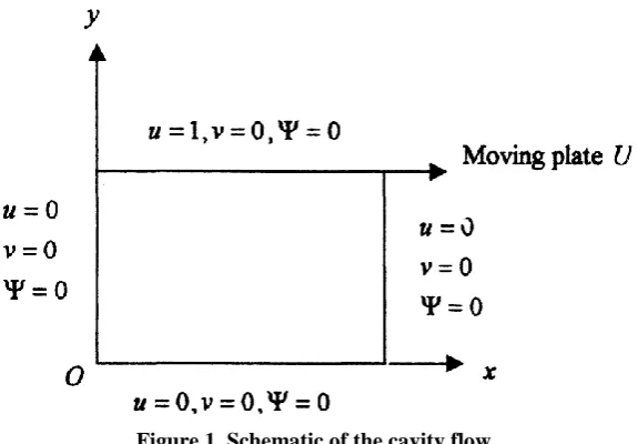
The problem considers incompressible flow in a cavity with an upper lid moving with a velocity U as shown in Figure 1.

Figure 1. Schematic of the cavity flow

The general non-dimensional, non conservative form of NSE:

    

  

                

    

  

                

     

2 2

Re 1

2 2

Re 1 0

y v

x v y

p y v v x v u t v

y u

x u x

p y u v x u u t u

y v x u

(3)

Application of certain mathematics operations on the Eqs, (1), (2) and (3) for the purpose of obtaining a Vorticity–Stream function formulation, the above equations are given in the following form as

                         2 2 2 2 Re 1 y x y v x u

t (2)













2 2 2 2

y

x



(3)

which are of parabolic and elliptic type, respectively.

An important advantage of this formulation is that pressure is not appeared in the above equations explicitly. So, the Vorticity–Stream function formulation does not contain the pressure term. x v y u      





,



(4)

                                      

 ₂ 2

2 2 2 2 2 2 2 2 2 y x y x y p x

p



(5)

Using numerical formulation of Vorticity-Stream function and employing the ADI scheme and Eq. (11), the velocity field is computed.

2.1. Discretization of vorticity equation

With regard to the fact that Eq. (4) is of parabolic type, this equation is discretized using the ADI scheme resulting in the efficient use of the nodes from the entire boundary. This provides high accuracy and more physical adaptation of the solution. More over with this scheme, three diagonal sets of equations are solved instead of five diagonal sets of equations. There is possibility of selection of better space and time steps and unconditional stability exists. Solution of ADI formulation gives the two following equations which are solved successively:

2 1 , , 1 , 2 , 1 , , 1 1 , 1 , , , 1 , 1 , , ,

)

(

2 Re

1 )

(

2 Re

1

2

2 /

)

(

2 1 2 1 2 1 2 1 2 1 2 1

y

x

y

V

x

U

t

n j i n j i n j i n j i n j i n j i n j i n j i n j i n j i n j i n j i n j i n j i

























































              (6-a) 2 1 1 , 1 , 1 1 , 2 , 1 , , 1 1 1 , 1 1 , , , 1 , 1 , , 1 ,

)

(

2 Re

1 )

(

2 Re

1

2

2 /

)

(

2 1 2 1 2 1 2 1 2 1 2 1 2 1 2 1

y

x

y

V

x

U

t

n j i n j i n j i n j i n j i n j i n j i n j i n j i n j i n j i n j i n j i n j i

























































                      (6-b)

(4)





n _x

j i x x n j i x n j i x

x

d

C

d

D

C

















_





















_



     2 1 2 1 2 1 , 1 , , 1

2

1

2

1

2

1

2

1

(7-a)





y

n j i y y n j i y n j i y

y

d

C

d

D

C

















_





















_



   

 ,11

1 , 1 1 ,

2

1

2

1

2

1

2

1

(7-b)

where the Courant and diffusion numbers are defined as

2 2 ) ( Re 1 , ) ( Re 1 , y t d x t d y t v C x t u C y x y x            

The right hand sides of Eq. (7) are defined respectively as





n

j i y y n j i y n j i y y

x C d d C d

D , 1 , , 1

2 1 2 1 1 2 1 2 1        _ _            _

 (8-a)





12 12

2 1 , 1 , , 1 2 1 2 1 1 2 1 2 1           _ _            _  n j i x x n j i x n j i x x

y C d d C d

D (8-b)

The values of u and v used in Eq. (7) could be used at time n or n+1/2. If the later time is taken, the stream function equation should be solved at time n+1/2, for which larger computation time will be utilized. Simplification of the above equations leads to

y n j i y n j i y n j i y x n j i x n j i x n j i x

D

C

B

A

D

C

B

A

























          2 1 2 1 2 1 2 1 2 1 2 1 1 , , 1 , , 1 , , 1 (9) in which

)

2

1 (

2

1

1 )

2

1 (

2

1 )

2

1 (

2

1

1 )

2

1 (

2

1

y y y y y y y y x x x x x x x x

d

C

d

B

d

C

A

d

C

d

B

d

C

A





























(10)

2.2. Discretization of stream function equation

Regarding that the stream function Eq. (3) is of elliptic type, the Guass Seidal point to point method is employed for solving this equation as

 

2





1 1 2 1

, 2 , 1, 1, , 1 , 1

1 2(1 )

k k k k k k

i j x i j i j i j i j i j



 





          _       _

(5)

in which y x   



(12)

Computation begins with solving the vorticity Eq. (6). Then, the vorticity in Eq. (11) is given

a new value and the stream function equation is solved for . This process is repeated until the

final convergent solution is achieved. After  computation, the velocity components are

computed using Eq. (4).

x

2 ψ

ψ

v

y

2 ψ

ψ

u

j 1, -i j 1, i j i, 1 -j i, 1 j i, j i,













  (13)

2.3. Discretization of poison equation

Computing the final flow field, in order to obtain pressure field, the poison Eq. (5) is discretized as follows;























2 2 2 2 2 2 2

)

(

)

(

)

(

2 y

x

y

x

p



(14)

This equation could be rewritten as

S P 2 (15) In which                                    2 2 2 2 2 2 2 y x y x

S



(16)

Therefore, we would have

                                                   2 1 , 1 1 , 1 1 , 1 1 , 1 2 1 , , 1 , 2 , 1 , , 1 , 4 ) ( 2 ) ( 2 2 y x y x S j i j i j i j i j i j i j i j i j i j i j i



(17)

Now, having Si,j and using the point by point Guass-Seidal elimination to discretize Eq. (15), pressure at all points of the flow domain is computed by







1



1 , 1 , 2 1 , 1 , 1 , 2 2 1 , ( ) ) 1 ( 2 1        _ _ _ _ _   k j i k j i k j i k j i k j i k j

i x s p p p p

p



(18)

2.4. Initial conditions

With regard to Figure 1, the initial conditions are defined as

0,

0

0 1,

0

1

(6)

2.5. Boundary conditions

The wall of the cavity is a stream line, and the stream function is constant on this surface and its value could be taken arbitrarily.

There is no explicit boundary condition for vorticity, so, boundary conditions should be constructed. The method for this purpose is the stream function equation and its Taylor series expansion. As a result, distinct formulations with different degrees of approximation are obtained. In this research, the first degree formulation is employed. With regard to Figure 1, the boundary conditions are defined as



                   xx x v u



0 0 0 JM j to 1 j : 1

i (20-a)



                   xx x v u



0 0 0 JM j to 1 j : IM

i (20-b)



                  yy y v u



0 0 0 IM i to 1 i : 1

j (20-c)



                  yy y v U u



0 0 IM i ا to 1 i : JM

j (20-d)

So, using certain mathematics for boundary conditions, the following relations are obtained for the boundaries.





 





 





 





 

y

U y y x x JMM i JM i JM i i i i j IMM j IM j IM j j j                   2 2 2 2 2 2 1 , , , 2 2 , 1 , 1 , 2 , 1 , , 2 , 2 , 1 , 1



(21)

(7)

are solved with the assumption that value of flow stream function on solid borders are zero. It should be mentioned that imposing boundary conditions of higher degrees leads to higher accuracy while causes instability in higher Reynolds numbers.

Eqs. (2) and (3) should be solved simultaneously. For this purpose, first the vorticity equation is solved, then, having the vorticity distribution, the poisson equation is solved for the stream function distribution. With stream function the boundary conditions of vorticity equation could be computed so that the vorticity equation could be solved for new solution at the next time-step. This process is repeated until the solution for the desired time is reached or the steady solution is achieved.

3. Results and Discussion

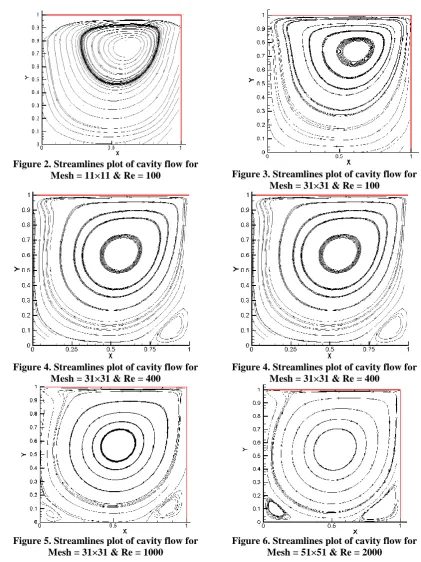
The fluid flow in a square cavity is the best problem to verify numerical results [4-7, 11]. Therefore flow field in a cavity was simulated. The velocity field at the top moving wall of the cavity shows a large recirculation region inside the cavity. With increasing moving wall velocity and the Reynolds number value, additional smaller recirculation zones appear in the corners of the cavity.

Figures 2 and 3 show the streamlines for Reynolds number 100 in two different computational grids of 31×31 and 11×11. As shown in Figures 4, 5 and 6, Computations are presented here for the Reynolds number 400 and 1000 in a 31×31 computational grid and for

Reynolds number 2000 in a 51×51 computational grid. The 11×11 computational grid is not able

(8)

Figure 2. Streamlines plot of cavity flow for

Mesh = 11×11 & Re = 100 Figure 3. Streamlines plot of cavity flow for Mesh = 31×31 & Re = 100

Figure 4. Streamlines plot of cavity flow for Mesh = 31×31 & Re = 400

(9)

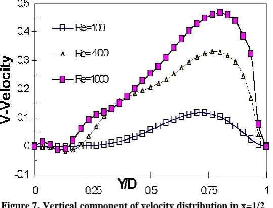
direction on the top is equal to the input value and at the solid boundary is zero. The vertical component is trivial compared with horizontal one due to swirling nature of flow. In other words the velocity fluctuations in the vertical direction are significantly higher than those in the horizontal direction.

Figure 7. Vertical component of velocity distribution in x=1/2

Figure 8 shows velocity field distribution at the centre of the cavity in x direction at y=D/2 (with D as the height of the cavity). On the solid boundary, the values of the velocity components are zero and the results show the nature and behavior of the flow very well.

Figure 8. Horizontal component of velocity distribution in y=D/2

(10)

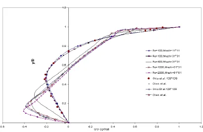
Figure 9. Comparison of vertical component of velocity distribution in x=L/2 with Ghia & Chen results

4. Conclusion

We have extended a vorticity-Stream function formulation for computation of unsteady incompressible fluid flow based on an alternating direction implicit. Therefore in this research, analysis of flow field in a cavity with different values of the Reynolds numbers 100, 400, 1000 and 2000 was carried out by solving the NSE using and Vorticity–Stream function formulation and the ADI algorithm. The solutions for wall cavity flow are stable and convergent. Moreover, we believe that more work need to be done in this subject. Therefore, we will try to solve this problem by using an ADI finite difference method. To this, special formulations with different degrees of approximation which satisfy the boundary conditions are obtained. Finally, comparing the results with the benchmarks show that alternating direction implicit is an effective and suitable formulation for the solution of NSE. Therefore the method is an efficient with promising results.

5. References

1. Ghia U, Ghia K N, Shin C T. (1982). High-Re solution for incompressible flow using the Navier-Stokes equations and a multigrid method. Journal of Computational Physics, 48(3), 387-411.

2. Chen KH, Pletcher RH, (1991), Primitive variable strongly implicit calculation procedure for viscous flows at all speeds. AIAA Journal, 29(8), 1241-1249.

3. Driesen C H, Kuerten J G M, Streng M. (1998). Low-Reynolds-number flow over partially covered cavities. Journal of Engineering Mathematics, 34(1-2), 3–21.

4. Koseff J R, Street R L. (1984). On end wall effects in a lid-driven cavity flow. Journal of Fluids Engineering, 106(4), 385–389.

(11)

quantitative observations. Journal of Fluids Engineering, 106(4), 390–398.

6. Prasad A K, Koseff J R. (1989). Reynolds number and end-wall effects on a lid-driven cavity flow. Physics of Fluids, 1(2), 208–218.

7. Aidun C K, Triantafillopoulos N G, Benson J D. (1991). Global stability of a lid-driven cavity with through flow: flow visualization studies. Physics of Fluids, 3(9), 2081–2091.

8. Gürcan F. (2003). Effect of the Reynolds number on streamline bifurcations in a double-lid-driven cavity with free surfaces. Computer & Fluids, 32(9), 1283–1298.

9. Erturk E, Gokcol O. (2007). Fine grid numerical solutions of triangular cavity flow. The European Physical Journal Applied Physics, 38(1), 97–105.

10. Agarwal R K. (1981). A third-order-accurate upwind scheme for Navier-Stokes solutions at high Reynolds numbers. AIAA Paper No. 81-0112, 15 p.