A language for modular spatio-temporal simulation.

(1)

E L S E V I E R Ecological Modelling 103 ( 1997 ) 105-113

|tBUNZnt

A language for modular spatio-temporal simulation

Tom Maxwell *, Robert Costanza

University of Maryland, Institute for Ecological Economics, Box 38, Solomons, MD 20 688, USA

Accepted 28 February 1997

Abstract

Creating an effective environment for collaborative spatio-temporal model development will require computational systems that provide support for the user in three key areas: (1) Support for modular, hierarchical model construction and archiving/linking of simulation modules; (2) support for graphical, icon-based model construction; (3) transparent, seamless support for state of the art distributed computing. The key requirement for this support is the adoption of a modeling standard, either in the form of an interface specification language (ISL), or a modular modeling language (MML). The ISL supports remote linking of simulation modules developed in disparate languages and environments. The MML provides a language standard for the development and archiving of simulation modules. Optimally, the implementation of these languages will include seamless links to graphical, icon-based simulation environments and distributed computing environments. In this paper we discuss the authors' program to develop and implement an MML-based integrated environment designed to provide this support for distributed modular spatio-temporal modeling. © 1997 Elsevier Science B.V.

Keywords: Modular; Hierarchical; Distributed; Spatial

I. Introduction

Protecting and preserving our natural life support systems requires the ability to understand the direct and indirect effects of h u m a n activities on these systems at multiple space-time scales. Our modeling and understanding o f these systems has

* Corresponding author. Tel.: + 1 410 3267388; e-mail: [email protected]; http:// kabir.cbl.cees.edu/Tom/ Maxwell.html

been largely isolated and unconnected in disciplinary specialties. There is great need for an integrated conceptual framework, as well as a practical toolbox allowing researchers f r o m m a n y disciplines to collaborate effectively to better understand the dynamics o f coupled environmental- economic systems. Supporting an inter- disciplinary research p r o g r a m o f this magnitude will require the development o f new modeling tools, data bases, and collaborative network infor- mation-sharing and simulation environments 0304-3800/97/$17.00 © 1997 Elsevier Science B.V. All rights reserved.

(2)

106 T. Maxwell, R. Costanza / Ecological Modelling 103 (1997) 105-113

to allow the linkage o f existing models and the evolution of a new set of modular, multi-faceted, adaptive models. In this paper we outline a number of these necessary advances and discuss current development efforts in this area.

2. Supporting collaborative modeling

Spatially explicit modeling of ecological-economic systems is essential if one's modeling goals include developing a relatively realistic description of past behavior and predictions of the impacts of alternative management policies on future system behavior (Risser et al., 1984; Costanza et al., 1990; Sklar and Costanza, 1991). There exists a rich set of research problems associated with the implementation of computer based collaborative technologies for spatially-articulated ecological economic modeling. Three important areas of on- going research and development are integrated support for: (1) modular, collaborative model development; (2) transparent access to high performance computing resources; (3) graphical display and manipulation of model structure and dynamics; and (4) integrating disparate spatio-temporal representations.

2.1. Collaborative, modular model development

One of the factors limiting the development of ecosystem models in general has been the inability of any single team of researchers to deal with the conceptual complexity of formulating, building, calibrating, and debugging complex models. The need for collaborative model building has been recognized (Goodall, 1974; Acock and Reynolds, 1990) in the environmental sciences. Realistic ecosystem models are becoming much too complex for any single group of researchers to implement single-handed, requiring collaboration between species specialists, hydrologists, chemists, land managers, economists, ecologists, and others. Communicating the structure of the model to others can become an insurmountable obstacle to collaboration and acceptance of the model.

A well-recognized method for reducing program complexity involves structuring the model as

a set of distinct modules with well-defined inter- faces (Gauthier and Ponto, 1970; Goodall, 1974; Acock and Reynolds, 1990; Silvert, 1993) Modu- lar design facilitates collaborative model construction, since teams of specialists can work independently on different modules with minimal risk of interference. Modules can be archived in distributed libraries and serve as a set of templates to speed future development. A modeling environment that supports modularity could provide a universal modeling language to promote global collaborative model development.

2.2. High performance computing

Tremendous computational resources are re- quired to integrate the equations of a large spatial model in a reasonable amount of computer time. Large models typically require supercomputers or parallel/distributed processing for efficient execu- tion. This class of models is a near ideal application for parallel processing since a typical model consists of a large number of cells that can be simulated semi-independently. Each processor can be assigned a different subset of cells, and most interprocessor communication is nearest-neighbor only. Despite their great promise and increasing availability, parallel architectures have not found much usage in the life sciences. The major barrier to wide acceptance of these techniques has been the difficulty of programming and debugging large parallel programs, and reluctance on the part of scientists to invest time in learning new languages and architectures

2.3. Graphical display

(3)

T. Maxwell. R. Costanza /Ecological Modelling 103 (1997) 105 113 107

ule dynamics. One major advantage of this graphical approach to modeling is that the process of modeling can become a consensus building tool. The graphical representation of the model can serve as a blackboard for group brainstorming, allowing policy makers, scientists, and stakehold- ers to all be involved in the modeling process. When applied in this manner the process of creating a model may be more valuable than the finished product.

3. Methods for supporting collaborative modeling

translate modules in other languages into MML for archiving and linking. The major advantage of this approach is that all modules can be archived and executed in a single unifying environment, which can provide extensive simulation services not found in a loosely coupled heterogeneous simulation. The modeling language should facilitate model development and communication be- cause it focuses on the issues of interest to the modelers while hiding unnecessary or dangerous implementation details, and encourages modular, hierarchical program design. We will discuss this approach for the remainder of this paper. There are two major methods for supporting

collaborative model construction, through implementation of a 'module wrapper', and through implementation of a 'modular modeling language'.

3.1. The module wrapper approach

This approach involves the development of a set of 'wrappers' which encapsulate legacy simulation code modules in order to integrate them into a single distributed environment, resulting in a 'federated' simulation. This wrapper is implemented as a library of functions (or distributed objects) that is embedded in the existing simulation codes to enable them to 'publish' (and 'sub- scribe to') simulation services over the network. Each module publishes its set of available services using a common high-level interface specification language, which is platform and programming language independent. The base infrastructure for implementing this approach is just becoming available with the advent of interoperability specifications such as CORBA (CORBA, 1996), and OGIS (OGIS, 1996). Significant infrastructure development remains to be done, however, before this approach become widely available.

3.2. Modular modeling language (MML)

This approach involves the utilization of a specialized language to support modular modeling. Modules can be developed, archived, and linked in this language. Converters can be created to

4. Properties of a modular modeling language and environment

A modular modeling language (MML) is only useful within the context of a modular modeling development environment (MMDE). The basic properties of a MML and MMDE are outlined here. For further reading on object oriented design methodology, consider the general references (Zeigler, 1976, 1990; Cook and Daniels, 1994; Erich Gamma et al., 1995; Robinson, 1996), as well as the environmental sciences references in Section 2.1.

4.1. Modular modeling language

Some of the key properties of a MML include: • Simplicity: the language should capture only details relevant to the dynamics of the model and leave all other computational details to the MMDE.

• Modularity: the separate components of the model should be represented in the language as a set of self-contained modules with well defined inputs and outputs. The module encap- sulates it's data and dynamics in the sense that it can only be interfaced through it's inputs and outputs.

(4)

108 T. Maxwell, R. Costanza / Ecological Modelling 103 (1997) 105-113

• Inheritance hierarchy: modules can subclass other modules. This allows modules to inherit some of the functionality (data and dynamics) of other modules while overriding other functionality. This property facilitates the construction of specialization hierarchies, in which each level of inheritance is composed of increasingly specialized modules.

• Connections: the language should include a method for declaring connections between modules (from output variables to input variables).

4.2. Modular modeling development environment

Some of the key properties of a MML-based development environment include:

• Graphical interface: the environment should provide a graphical interface to the MML, in which each element is represented by an icon, and inter-element connections are displayed graphically. Scientists unfamiliar with the environment should be able to begin building and running models almost immediately; the interface should be largely self-explanatory. • Simulation services: the modeling environment

should provide a number of user-transparent simulation services. These services should include: (i) modeling toolbox, tools for integrating differential equations, performing sensitivity analyses, and displaying the model output graphically in various forms, as well as providing math tools to support model building; (ii) network toolbox, tools for automatically distributing the simulation over a network of processors; and (iii) data access/storage utili- ties, tools for seamlessly linking to GIS/data- bases for simulation data input and output.

5. Spatial modeling language

In an attempt to address the conceptual and computational complexity barriers to spatio-temporal model development, we have implemented a realization of the MML and MMDE specifications (detailed in Section 4) which we call the spatial modeling language (SML) and the spatial

modeling environment (SME). The SML is described in this section, and the SME is described in Section 6.

5.1. Description of the S M L

The spatial modeling language (SML) is a data- parallel simulation design language designed to support modular simulation by incorporating the MML specifications outlined in Section 4.1. It is structured as a set of nested object definitions and attribute-value declarations. The declarative structure of the SML is described in this section, the SML infrastructure for handling spatial interac- tion is described in Section 6.

5. I. 1. Object definitions

The general form of a object definition in SML is:

< modifiers > < objectType > < objectName > : < parentObjectName >

where < objectName > is the name of the object, < objectType > is the type of the object, and < parentObjectName > is the name of the object that this object inherits from. Each command also accepts a set of modifiers, which denote special- izations of the declared object. Each object declaration can optionally be followed by a definition of the declared object, which is enclosed in brack- ets. Object definitions may contain declarations and definitions of other objects.

5.1.2. Attribute-value declarations

The general form of a attribute-value declaration in SML is:

< modifiers > < objectType > < objectName > = < value >

(5)

T. Maxwell, R. Costanza /Ecological Modelling 103 (1997) 105 113 109

5.1.3. SML object types

The object types supported by the current version of the SML include:

(1) Module: the module object is the unit of encapsulation of the model dynamics. Modules are designed to be self-contained archivable sub- models, which may interact with other modules through well-defined input and output ports. Module declarations may be nested to arbitrary depth, and modules may inherit from other modules.

(2) Variable: variable objects represent the atomic components of a module. Command qualifiers can be used to specify specific variable sub-classes, such as state variable, flux variable, map-dependent parameter, timeSeries, spatially interpolated timeSeries, and parameter.

(3) Frame: a frame object specifies the topology of the spatial implementation of a module. Frames are discussed in Section 6.

(4) Connection: a connection object establishes a link from an output variable in one module to an input variable in another module.

(5) Input: each module may declare a set of input ports. These ports behave as local variables within the module, i.e. they appear within the module's dynamic equations as variables declared within the module. Each port is connected to an output variable in another module. At the begin- ning of each update event, data is imported through each referenced port from the connected output variable and remapped (if necessary) into the importing module's frame.

(6) Event: the simulation is driven by a set of events. An event object contains a timestamp and a list of commands to be executed, sorted by dependency. Events are posted to a global list which is sorted by timestamp. The events in the list are executed sequentially to generate the dynamics of the simulation. When an event is executed the following steps occur: (ii) the global simulation time is set equal to the event's timestamp; (ii) the Event's Commands are executed; and (iii) the event uses it's schedule object to reschedule itself.

(7) Schedule: the schedule object controls the scheduling of Events. Schedules are arranged in a hierarchical structure, with variables inheriting

schedules from their modules and sub-modules inheriting schedules from super-modules. At any level of the hierarchy a schedule may be re- configured, overriding aspects of it's inherited schedule.

(8) Command: the atomic components of an event are command objects. Each command object is designed to perform a single 'action'. The currently supported command classes include: (i) update: update a variable's data structures, either by executing a set of equations of by importing data from another module; (ii) script: execute a script in the shell environment; (iii) pipe: execute a pipe operation.

(9) Pipe: all data input and output is performed using pipes. A pipe object links a variable object with an external data source/sink/display object. pipes exist for: (i) importing data from the GIS or database; (ii) archiving data to the GIS or database; and (iii) displaying data in real time using various formats.

5.2. An SML example

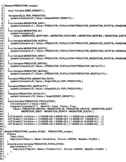
The SML code in lines 1-49 of Fig. 1 represents the declaration and definition of a simple module implementing predator dynamics (with migration). The line numbers in Fig. 1 were added for reference purposes, and are not part of the language. The SML code was imported from a set of equations generated using a graphical modeling tool such as STELLA. The module has a set of variable objects (declared with the variable command), which can be internal, or input from another module (declared with the input modifier, as in line 3). All internal variables can serve as exports to other modules. Each variable has an associated set of command declarations, which define the operations that are used to update the variable's values (as described in Section 6.4). The SME code generator automatically associates commands with events, which subsequently drive the simulation. The user may override the default event structure by defining a set of customized events if necessary.

(6)

110 T. Maxwell, R. Costanza / Ecological Modelling 103 (1997) 105-113

Fig. 1. An SML example.

defined) PREDATORS_module by adapting it to a specific study area. A frame is declared (lines 52-55) to specify the topology of the module. The initialization command ill for the predator state variable (line 40) is overridden by a map input pipe (lines 56-59) in order to specify the initial distribution of predators. This is accomplished by 'extending' the P R E D A T O R _ P O P U L A T I O N state variable declaration (line 56).

6. Spatial modeling environment

In an attempt to address the conceptual and computational complexity barriers to spatio-temporal model development, we have implemented a realization of the M M D E specification (detailed in Section 4) which we call the spatial modeling environment (SME) (Maxwell, 1994; Maxwell and Costanza, 1994, 1995). The spatial modeling language (SML) forms the core of (SME), which links icon-based graphical modeling environments with parallel supercomputers and a generic object database. This system will allow users to create and share modular, reusable model components, and utilize advanced parallel computer architectures without having to invest unnecessary time in

computer programming or learning new systems. The SME is described elsewhere (references above) in this paper we discuss only the aspects of the SME/SML which support spatial interactions.

6. I. The S M E driver

The SME driver is the distributed object-oriented simulation environment which incorporates the set of code modules that actually perform the spatial simulation. The SME code generator will convert an SML object hierarchy (typically developed using one of the SME/SML graphical model development tools) into a C + + object hierarchy which is incorporated into the SME driver application. The simulation is executed within the SME, which provides numerous simulation services such as transparent distributed computing, integrated visualization and analysis tools, and integrated GIS and database access.

6.2. Spatial representations: the PointGrid library

(7)

uses to build spatial representations. The P G L object structure is a mapping of (a subset of) an early version of the OG1S Open Geodata Model (OGIS, 1996) to C + + .

The P G L supports spatial representations as sets of Point objects (see below) with links. It transparently handles: (1) creation and decomposition (over processors) of Point Sets; (2) mapping of data over and between Point Sets; (3) iteration over Point Sets and Point Sub-Sets; (4) data access and update at each Point; and (5) swapping of variable-sized PointSet boundary (ghost) re- gions. Some of the important P G L classes are: • Point: corresponds to a cell in a GIS layer. • Aggregated point: corresponds to a cell in a

coarser resolution GIS layer.

• PointSet: a set of Points with (optional) links (grid, network, tree, population, etc.).

• DistributedPointSet: a PointSet distributed over processors with variable-sized boundary (ghost) layers.

• Coverage: one-to-one mapping from a Dis- tributedPointSet to the set of floating point numbers.

6.3. Modules and frames

Each module that is declared in the SML has a frame object that is used to configure the spatial representation of the module in the driver. All variable objects belonging to a module inherit the module's frame. The SME provides a set of available frame types, which currently includes 2D grids, networks, and trees. The user specifies a frame type and a frame configuration map (to be read from the GIS at runtime) for each module. The frame object is implemented in the driver as a DistributedPointSet object, i.e. each frame has a list of Point objects (POs), with each PO corresponding to a cell in the frame's map region, which includes a partition of the study area han- dled by the current processor plus a communication buffer zone. Every frame object in the SME includes methods for interacting with and trans- ferring data to/from other frames. The SML spatial variable object is implemented as a coverage object, i.e. each variable object in the driver contains a mapping from it's (module's) frame to the set of floats.

6.4. Defining spatial interactions in the S M L

Dynamic variables in the SML fall into two general classes: (1) spatial variables, which (at any point in time) have a different value at each cell of the frame; and (2) non-spatial variables, which have a single value in all cells. All operations on spatial variables (e.g. command u2 in Fig. 1, lines 12-14) are executed in a 'data parallel' mode. This means that an operation defined as A + B (where A, and B are spatial variables) results in a separate addition operation for each cell of the frame, using the variable values associated with that cell.

Defining the intercellular interactions requires an additional syntax. In any SML equation, a term defined as S@(x, y) (where S is a spatial variable with a grid frame, and x and y are integers) represents the value of S x cells to the north and y cells to the east. This syntax has a similar meaning in other frames. Fig. 1, line 12 shows an example of predator migration dynamics defined using this notation. We are currently developing an additional set of operators to declare common spatial operations, such as convo- lutions and spatial averages.

7. Patuxent landscape model example application

(8)

112 T. Maxwell, R. Costanza / Ecological Modelling 103 (1997) 105-113

6 7 8 9 10 11 12 13 14 15 161 17 18 19 20 21 22 23 24 25 26 27 28 29 3O 31 32 33 34 35 36 37 38 39 40 41 42 43 44 45 46 47 48 49 5O 51 5 2 53 54! 5 s 5 6 57i 5Bi 5 9 6O 61 62

Module PREDATORS_module {

input Variable DEERDENSITY { }

Variable KILLS_PER_PREDATOR {

update Command u0 { Value = Graph0(DEER_DENSITY); } }

f I u x Variable MIGRATION_EAST {

update Command u I { Value = PREDATOR_POPULATION*PREDATOR_MIGRATION RATE*SL::RANDOM(0.1,0.4); } )

f I u x Variable MIGRATION_IN { update Command u2 {

Value -- MIGRATION_NORTH@S + MIGRATION_SOUTH@N + MIGRATION_WEST@E + MIGRATION_EAST@W; } )

f I u x Variable MIGRATION NORTH {

update Command u3 { Value = PREDATOR_POPULATION*PREDATOR_MIGRATION_RATE*SL::RANDOM(0.1,0.4); } )

f I u x Variable MIGRATION_SOUTH {

update Command u4 { Value -- PREDATOR_POPULATION*PREDATOR_MIGRATION_RATE*SL::RANDOM(0.1,0.4); } }

f I u x Variable MIGRATION_WEST {

update Command u5 { Value = PREDATOR_POPULATION'PREDATOR_MIGRATION_RATE*SL::RANDOM(0.1,0.4); } }

f l u x Variable PREDATORBIRTHS {

update Command u6 { Value = (PREDATOR_POPULATION*PREDATOR_NATALITY); } }

f I u x Variable PREDATOR_DEATHS {

update Command u7 { Value = (PREDATOR_POPULATION*PREDATOR_MORTAUTY); } }

Variable PREDATORMIGRATION_RATE {

update Command u8 { Value = Graphl(KILLS_PER_PREDATOR); } }

Variable PREDATOR_MORTALITY {

update Command u9 { Value = Graph2(KILLS_PER_PREDATOR); } }

Variable PREDATOR_NATALITY {

update Command ul 0 { Value = Graph3(DEER DENSITY); } }

s t a t e Variable PREDATORPOPULATION { init Command il I { Value = 3000; }

integrateCommand111{ Method= Euler; Clamp= True;

Value = PREDATOR_BIRTHS + MIGRATION IN- PREDATORDEATHS- MIGRATION_EAST- MIGRATION_WEST- MIGRATION_NORTH- MIGRATION_SOUTH; }

}

LUT G raph0 { l i st Data = ( ( 0.0000E+00, 0.0000E+00 ), ( 1.0000E+00, 4.0000E-02 ), ...) } LUT Graph1 { list Data = ( ( 0.0000E+00, 1.0000E+00 ), ( 4.0000E-01,7.9500E-01 ), ...) } LUT Graph2 { list Data = ( ( 0.0000E+00, 1.0000E+00 ), ( 1.5000E-01,8.0000E-01 ), ...) } LUT Graph3 { list Data = ( ( 0.0000E+00, 5.0000E-02 ), ( 1.0000E+01,5.0000E-02 ), ...) } }

Module PREDATORS_module_PLM25 : PREDATORS_module { Frame {

Type = Grid;

map i m p o r t Pipe p l { Name = StudyArea; Source = GRASS; MapSet = PLM25; } }

extends s t a t e Variable PREDATOR_POPULATION { pipe Command il 1 {

map i m p o r t Pipe p2 { Name = P r e d a t o r l n i t l ; Source = GRASS; MapSet = PLM25; } }

} }

(9)

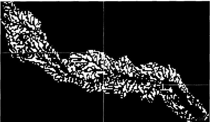
display a decomposition of the PLM grid frame over four processors as generated by the SME driver using a recursive N-section algorithm. Ap- plication of this model in the Patuxent watershed is expected to allow extensive analysis of past and future management options, and will form the basis for future application to other areas in the Chesapeake Bay watershed.

8. Conclusions

We believe that effectively managing human affairs through the next century will require ex- tremely complex and reliable computer models. Widespread utilization of modeling environments supporting graphical, hierarchical/modular design of distributed simulations will facilitate reliable, economical model construction. General adoption of this paradigm will support the development of libraries of modules representing reusable model components that are globally available to model builders, as well as making advanced computing architectures available to users with little computer knowledge.

References

Acock, B., Reynolds, J.F., 1990. Model Structure and Data Base Development. In: Dixon R.K., Meldahl R.S., Ruark G.A., Warren W.G. (Eds.), Process Modeling of Forest Growth Responses to Environmental Stress. Timber Press, Portland, OR.

Cook, S., Daniels, J., 1994. Designing Object Systems. Prentice Hall, New York.

CORBA, 1996. Object Management Group. URL: http:// www.omg.org/.

Costanza, R., Sklar, F.H., White, M.L., 1990. Modeling coastal landscape dynamics. BioScience 40, 91 107. ELM, 1995. Everglades Landscape Model. URL: http://

kabir.umd.edu /Glades/ELM.html.

Erich Gamma, R.H., Johnson, R., Vlissides, J., 1995. Design Patterns: Elements of Reusable Object-Oriented Software. Addison-Wesley, Reading, Massachusettss.

Fitz, H.C., DeBellevue, E., Costanza, R., Boumans, R., Maxwell, T., Wainger, L., 1996. Development of a general ecosystem model (GEM) for a range of scales and ecosys- tems. Ecol. Model. 88, 263 297.

Gauthier, R.L., Ponto, S.D., 1970. Designing Systems Pro- grams. Prentice-Hall, Englewood Cliffs, NJ.

Goodall, D.W., 1974. The Hierarchical Approach to Model Building. Center for Agricultural Publishing and Docu- mentation, Wageningen.

Maxwell, T., 1994. Distributed Modular Spatial Ecosystem Modelling.

Maxwell, T., Costanza, R., 1994. Spatial Ecosystem Modeling in a Distributed Computational Environment. In: van den Bergh, J., van der Straaten, J. (Eds.), Toward Sustainable Development: Concepts, Methods, and Policy. Island Press, Washington, D.C.

Maxwell, T., Costanza, R., 1995. Distributed modular spatial ecosystem modelling. Int. J. Comput. Simulation: Special Issue on Advanced Simulation Methodologies 5 (3), 247- 262.

OGIS, 1996. The OpenGIS Guide. URL: http://ogis.org/ guide/gnidel .htm.

PLM, 1995. Integrated Ecological Economic Modeling. URL: http://kabir.umd.edu/PLM/PLM Proj.html.

Risser, P.G., Karr, J.R., Forman, R.T.T., 1984. Landscape Ecology: Directions and Approaches. Illinois Natural His- tory Survey, Champaign, IL.

Robinson, P., 1996. Hierarchical Object-Oriented Design. Prentice Hall, New York.

Silvert, W., 1993. Object-oriented ecosystem modeling. Ecol. Model. 68, 91 118.

Sklar, F.H., Costanza, R., 1991. The Development of Dy- namic Spatial Models for Landscape Ecology. In: Turner, M.G., Gardner, R. (Eds.), Quantitative Methods in Land- scape Ecology. Springer-Verlag, New York, NY. Zeigler, B.P., 1976. Theory of Modeling and Simulation. Wi-

ley, New York.