Improving CUR Matrix Decomposition and the Nystrom Approximation via Adaptive Sampling

(1)

Improving CUR Matrix Decomposition and the Nystr¨om

Approximation via Adaptive Sampling

Shusen Wang [email protected]

College of Computer Science and Technology Zhejiang University

Hangzhou, Zhejiang 310027, China

Zhihua Zhang∗ [email protected]

Department of Computer Science and Engineering Shanghai Jiao Tong University

800 Dong Chuan Road, Shanghai, China 200240

Editor:Mehryar Mohri

Abstract

The CUR matrix decomposition and the Nyström approximation are two important low-rank matrix approximation techniques. The Nyström method approximates a symmetric positive semidefinite matrix in terms of a small number of its columns, while CUR approximates an arbitrary data matrix by a small number of its columns and rows. Thus, CUR decomposition can be regarded as an extension of the Nyström approximation.

In this paper we establish a more general error bound for the adaptive column/row sampling algorithm, based on which we propose more accurate CUR and Nyström algorithms with expected relative-error bounds. The proposed CUR and Nyström algorithms also have low time complexity and can avoid maintaining the whole data matrix in RAM. In addition, we give theoretical analysis for the lower error bounds of the standard Nyström method and the ensemble Nyström method. The main theoretical results established in this paper are novel, and our analysis makes no special assumption on the data matrices.

Keywords: large-scale matrix computation, CUR matrix decomposition, the Nystr¨om method,

randomized algorithms, adaptive sampling

1. Introduction

Large-scale matrices emerging from stocks, genomes, web documents, web images and videos everyday bring new challenges in modern data analysis. Most efforts have been focused on manipu-lating, understanding and interpreting large-scale data matrices. In many cases, matrix factorization methods are employed for constructing parsimonious and informative representations to facilitate computation and interpretation. A principled approach is the truncated singular value decompo-sition (SVD) which finds the best low-rank approximation of a data matrix. Applications of SVD such as eigenfaces (Sirovich and Kirby, 1987; Turk and Pentland, 1991) and latent semantic analysis (Deerwester et al., 1990) have been illustrated to be very successful.

(2)

However, using SVD to find basis vectors and low-rank approximations has its limitations. As pointed out by Berry et al. (2005), it is often useful to find a low-rank matrix approximation which posses additional structures such as sparsity or nonnegativity. Since SVD or the standard QR decomposition for sparse matrices does not preserve sparsity in general, when the sparse matrix is large, computing or even storing such decompositions becomes challenging. Therefore it is useful to compute a low-rank matrix decomposition which preserves such structural properties of the original data matrix.

Another limitation of SVD is that the basis vectors resulting from SVD have little concrete meaning, which makes it very difficult for us to understand and interpret the data in question. An example of Drineas et al. (2008) and Mahoney and Drineas (2009) has well shown this viewpoint; that is, the vector[(1/2)age₋(1/√2)height+ (1/2)income], the sum of the significant uncorrelated features from a data set of people’s features, is not particularly informative. Kuruvilla et al. (2002) have also claimed: “it would be interesting to try to find basis vectors for all experiment vectors, using actual experiment vectors and not artificial bases that offer little insight.” Therefore, it is of great interest to represent a data matrix in terms of a small number of actual columns and/or actual rows of the matrix.Matrix column selectionand theCUR matrix decompositionprovide such techniques.

1.1 Matrix Column Selection

Column selection has been extensively studied in the theoretical computer science (TCS) and nu-merical linear algebra (NLA) communities. The work in TCS mainly focuses on choosing good columns by randomized algorithms with provable error bounds (Frieze et al., 2004; Deshpande et al., 2006; Drineas et al., 2008; Deshpande and Rademacher, 2010; Boutsidis et al., 2011; Gu-ruswami and Sinop, 2012). The focus in NLA is then on deterministic algorithms, especially the rank-revealing QR factorizations, that select columns by pivoting rules (Foster, 1986; Chan, 1987; Stewart, 1999; Bischof and Hansen, 1991; Hong and Pan, 1992; Chandrasekaran and Ipsen, 1994; Gu and Eisenstat, 1996; Berry et al., 2005). In this paper we focus on randomized algorithms for column selection.

Given a matrixA_∈Rm×n, column selection algorithms aim to chooseccolumns ofAto con-struct a matrixC_∈_Rm×c _{such that}_k_A₋_CC†_A_k

ξachieves the minimum. Here “ξ=2,” “ξ=F,” and “ξ=_∗” respectively represent the matrix spectral norm, the matrix Frobenius norm, and the matrix nuclear norm, andC†denotes the Moore-Penrose inverse ofC. Since there are(n

c)possible

choices of constructingC, selecting the best subset is a hard problem.

In recent years, many polynomial-time approximate algorithms have been proposed. Among them we are especially interested in those algorithms with multiplicative upper bounds; that is, there exists a polynomial function f(m,n,k,c)such that withc(_≥k)columns selected fromAthe following inequality holds

kA₋CC†A_k_ξ _≤ f(m,n,k,c)_kA₋Akkξ

(3)

However, the column selection method, also known as the A_≈CX decomposition in some applications, has its limitations. For a large sparse matrix A, its submatrixC is sparse, but the coefficient matrixX_∈Rc×nis not sparse in general. TheCXdecomposition suffices whenm_≫n, becauseXis small in size. However, whenmandnare near equal, computing and storing the dense matrixXin RAM becomes infeasible. In such an occasion the CUR matrix decomposition is a very useful alternative.

1.2 The CUR Matrix Decomposition

The CUR matrix decomposition problem has been widely discussed in the literature (Goreinov et al., 1997a,b; Stewart, 1999; Tyrtyshnikov, 2000; Berry et al., 2005; Drineas and Mahoney, 2005; Mahoney et al., 2008; Bien et al., 2010), and it has been shown to be very useful in high dimensional data analysis. Particularly, a CUR decomposition algorithm seeks to find a subset ofccolumns of

Ato form a matrixC_∈Rm×c, a subset ofrrows to form a matrix R_∈Rr×n, and an intersection matrixU_∈Rc×r_{such that}_k_A₋_CUR_k

ξis small. Accordingly, we use ˜A=CURto approximateA.

Drineas et al. (2006) proposed a CUR algorithm with additive-error bound. Later on, Drineas et al. (2008) devised a randomized CUR algorithm which has relative-error bound w.h.p. if suffi-ciently many columns and rows are sampled. Mackey et al. (2011) established a divide-and-conquer method which solves the CUR problem in parallel. The CUR algorithms guaranteed by relative-error bounds are of great interest.

Unfortunately, the existing CUR algorithms usually require a large number of columns and rows to be chosen. For example, for anm×nmatrixAand a target rankk≪min{m,n},the subspace sam-pling algorithm(Drineas et al., 2008)—a classical CUR algorithm—requires

O

_(k_ε−2_log_k)_columns

and

O

_(k_ε−4_log2_k) _{rows to achieve relative-error bound w.h.p. The subspace sampling algorithm}

selects columns/rows according to the statistical leverage scores, so the computational cost of this algorithm is at least equal to the cost of the truncated SVD ofA, that is,

O

_(mnk)_{in general.}

How-ever, maintaining a large scale matrix in RAM is often impractical, not to mention performing SVD. Recently, Drineas et al. (2012) devised fast approximation to statistical leverage scores which can be used to speedup the subspace sampling algorithm heuristically—yet no theoretical results have been reported that the leverage scores approximation can give provably efficient subspace sampling algorithm.

The CUR matrix decomposition problem has a close connection with the column selection prob-lem. Especially, most CUR algorithms such as those of Drineas and Kannan (2003); Drineas et al. (2006, 2008) work in a two-stage manner where the first stage is a standard column selection pro-cedure. Despite their strong resemblance, CUR is a harder problem than column selection because “one can get good columns or rows separately” does not mean that one can get good columns and rows together. If the second stage is na¨ıvely solved by a column selection algorithm onAT, then the approximation factor will trivially be√2f1 (Mahoney and Drineas, 2009). Thus, more sophisticated error analysis techniques for the second stage are indispensable in order to achieve relative-error bound.

1. It is becausekA₋CUR_k2

F =kA−CC†A+CC†A−CC†AR†Rk2F =k(I−CC†)Ak2F+kCC†(A−AR†R)k2F ≤ kA−CC†Ak2

(4)

1.3 The Nystr¨om Methods

The Nyström approximation is closely related to CUR, and it can potentially benefit from the ad-vances in CUR techniques. Different from CUR, the Nyström methods are used for approximating symmetric positive semidefinite (SPSD) matrices. The methods approximate an SPSD matrix only using a subset of its columns, so they can alleviate computation and storage costs when the SPSD matrix in question is large in size. In fact, the Nyström methods have been extensively used in the machine learning community. For example, they have been applied to Gaussian processes (Williams and Seeger, 2001), kernel SVMs (Zhang et al., 2008), spectral clustering (Fowlkes et al., 2004), ker-nel PCA (Talwalkar et al., 2008; Zhang et al., 2008; Zhang and Kwok, 2010), etc.

The Nystr¨om methods approximate any SPSD matrix in terms of a subset of its columns. Specif-ically, given anm_×mSPSD matrixA, they require samplingc(<m) columns ofAto construct an m_×cmatrixC. Since there exists anm_×mpermutation matrixΠsuch thatΠCconsists of the first ccolumns ofΠAΠT_{, we always assume that}_C_{consists of the first}_c_{columns of}_A_{without loss of}

generality. We partitionAandCas

A =

W AT₂₁

A21 A22

and C =

W A21

,

whereWandA21are of sizesc×cand(m−c)×c, respectively. There are three models which are

defined as follows.

• The Standard Nystr¨om Method. The standard Nystr¨om approximation toAis

˜

Anys_c = CW†CT =

W AT₂₁

A21 A21W†AT21

. (1)

HereW†_{is called the}_{intersection matrix. The matrix}₍_W

k)†, wherek≤candWk is the best

k-rank approximation toW, is also used as an intersection matrix for constructing approxi-mations with even lower rank. But using W† results in a tighter approximation than using (Wk)†usually.

• The Ensemble Nystr¨om Method(Kumar et al., 2009). It selects a collection oftsamples,

each sampleC(i), (i=1,_···,t), containingccolumns ofA. Then the ensemble method com-bines the samples to construct an approximation in the form of

˜

A_tens_,_c =

t

∑

i=1

µ(i)C(i)W(i)†C(i)T, (2)

whereµ(i)_{are the weights of the samples. Typically, the ensemble Nystr¨om method seeks} to find out the weights by minimizing_kA₋A˜ens

t,ckF orkA−A˜enst,ck2. A simple but effective

strategy is to set the weights asµ(1)=_···=µ(t)=1 t.

• The Modified Nystr¨om Method(proposed in this paper). It is defined as

˜

Aimp_c = C C†A(C†)TCT.

(5)

flops to compute matrix multiplications. The matrix multiplications can be executed very efficiently in multi-processor environment, so ideally computing the intersection matrix costs time only linear inm. This model is more accurate (which will be justified in Section 4.3 and 4.4) but more costly than the conventional ones, so there is a trade-off between time and accuracy when deciding which model to use.

Here and later, we call those which use intersection matrixW†or(Wk)†the conventional Nystr¨om

methods, including the standard Nystr¨om and the ensemble Nystr¨om.

To generate effective approximations, much work has been built on the upper error bounds of the sampling techniques for the Nystr¨om method. Most of the work, for example, Drineas and Mahoney (2005), Li et al. (2010), Kumar et al. (2009), Jin et al. (2011), and Kumar et al. (2012), studied the additive-error bound. With assumptions on matrix coherence, better additive-error bounds were ob-tained by Talwalkar and Rostamizadeh (2010), Jin et al. (2011), and Mackey et al. (2011). However, as stated by Mahoney (2011), additive-error bounds are less compelling than relative-error bounds. In one recent work, Gittens and Mahoney (2013) provided a relative-error bound for the first time, where the bound is in nuclear norm.

However, the error bounds of the previous Nyström methods are much weaker than those of the existing CUR algorithms, especially the relative-error bounds in which we are more interested (Mahoney, 2011). Actually, as will be proved in this paper, the lower error bounds of the standard Nyström method and the ensemble Nyström method are even much worse than the upper bounds of some existing CUR algorithms. This motivates us to improve the Nyström method by borrowing the techniques in CUR matrix decomposition.

1.4 Contributions and Outline

The main technical contribution of this work is the adaptive sampling bound in Theorem 5, which is an extension of Theorem 2.1 of Deshpande et al. (2006). Theorem 2.1 of Deshpande et al. (2006) bounds the error incurred by projection onto column or row space, while our Theorem 5 bounds the error incurred by the projection simultaneously onto column space and row space. We also show that Theorem 2.1 of Deshpande et al. (2006) can be regarded as a special case of Theorem 5.

More importantly, our adaptive sampling bound provides an approach for improving CUR and the Nystr¨om approximation: no matter which relative-error column selection algorithm is employed, Theorem 5 ensures relative-error bounds for CUR and the Nystr¨om approximation. We present the results in Corollary 7.

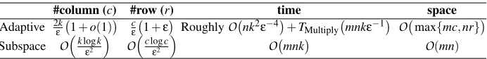
Based on the adaptive sampling bound in Theorem 5 and its corollary 7, we provide a concrete CUR algorithm which beats the best existing algorithm—the subspace sampling algorithm—both theoretically and empirically. The CUR algorithm is described in Algorithm 2 and analyzed in Theorem 8. In Table 1 we present a comparison between our proposed CUR algorithm and the subspace sampling algorithm. As we see, our algorithm requires much fewer columns and rows to achieve relative-error bound. Our method is more scalable for it works on only a few columns or rows of the data matrix in question; in contrast, the subspace sampling algorithm maintains the whole data matrix in RAM to implement SVD.

Another important application of the adaptive sampling bound is to yield an algorithm for the modified Nystr¨om method. The algorithm has a strong relative-error upper bound: for a target rank k, by sampling2_εk2 1+o(1)

(6)

#column (c) #row (r) time space

Adaptive 2_εk 1+o(1) c

ε 1+ε

RoughlyO nk2ε−4₊_T

Multiply mnkε−1 _O

max{mc,nr}

Subspace Oklogk ε2

Oclogc ε2

O _mnk O₍_mn₎

Table 1: Comparisons between ouradaptive samplingbased CUR algorithm and the best existing algorithm—thesubspace samplingalgorithm of Drineas et al. (2008).

kA₋A˜_kF

maxi,j|ai j|

kA₋A˜_k2 maxi,j|ai j|

kA₋A˜_k_∗

maxi,j|ai j|

kA₋A˜_kF

kA−AkkF

kA₋A˜_k2 kA−Akk2

kA₋A˜_k_∗ kA−Akk∗

Standard Ω m√k c

Ω m

c

Ω m₋c Ωq1+mk_c2

Ω m

c

Ω 1+k_c

Ensemble Ω m√k c

– Ω m−c Ωq1+mk

c2

– Ω 1+k

c

Table 2: Lower bounds of the standard Nystr¨om method and the ensemble Nystr¨om method. The blanks indicate the lower bounds are unknown to us. Here m denotes the column/row number of the SPSD matrix,cdenotes the number of selected columns, andkdenotes the target rank.

Finally, we establish a collection of lower error bounds of the standard Nyström and the ensem-ble Nyström that useW†as the intersection matrix. We show the lower bounds in Theorem 12 and Table 3; here Table 2 briefly summarizes the lower bounds in Table 3. From the table we can see that the upper error bound of our adaptive sampling algorithm for the modified Nyström method is even better than the lower bounds of the conventional Nyström methods.2

The remainder of the paper is organized as follows. In Section 2 we give the notation that will be used in this paper. In Section 3 we survey the previous work on the randomized column selection, CUR matrix decomposition, and Nystr¨om approximation. In Section 4 we present our theoretical results and corresponding algorithms. In Section 5 we empirically evaluate our proposed CUR and Nystr¨om algorithms. Finally, we conclude our work in Section 6. All proofs are deferred to the appendices.

2. Notation

First of all, we present the notation and notion that are used here and later. We letImdenote the

m_×midentity matrix,1mdenote them×1 vector of ones, and0denote a zero vector or matrix with

appropriate size. For a matrixA= [ai j]∈Rm×n, we leta(i)be itsi-th row,aj be itsj-th column, and

Ai:j be a submatrix consisting of itsito j-th columns (i≤ j).

Letρ=rank(A)_≤min_{m,n_}andk_≤ρ. The singular value decomposition (SVD) ofAcan be written as

A=

ρ

∑

i=1

σA,iuA,ivTA,i=UAΣAVTA=

UA,k UA,k⊥

ΣA,k 0

0 ΣA,k⊥

VT_A,_k VT_A,_k_⊥

,

(7)

whereUA,k (m×k),ΣA,k(k×k), andVA,k (n×k) correspond to the topksingular values. We denote

Ak=UA,kΣA,kV_A,T_k which is the best (or closest) rank-kapproximation toA. We also useσi(A) = σA,ito denote thei-th largest singular value. WhenAis SPSD, the SVD is identical to the eigenvalue

decomposition, in which case we haveUA=VA.

We define the matrix norms as follows. Let_kA_k1=∑i,j|ai j|be theℓ1-norm,kAkF= (∑i,ja2i j)1/2=

(∑iσ2A,i)1/2be the Frobenius norm,kAk2=maxx_∈Rn_,_k_x_k

2=1kAxk2=σA,1be the spectral norm, and kA_k∗=∑iσA,ibe the nuclear norm. We always usek · kξto representk · k2,k · kF, ork · k∗.

Based on SVD, the statistical leverage scoresof the columns ofArelative to the best rank-k approximation toAis defined as

ℓ[_jk]=v(_A,j)_k2

2, j=1,···,n. (3)

We have that∑nj=1ℓ

[k]

j =k. The leverage scores of the rows ofAare defined according toUA,k. The

leverage scores play an important role in low-rank matrix approximation. Informally speaking, the columns (or rows) with high leverage scores have greater influence in rank-k approximation than those with low leverage scores.

Additionally, let A†=VA,ρΣ_A,−1_ρUT_A,ρbe the Moore-Penrose inverse ofA(Ben-Israel and Gre-ville, 2003). WhenAis nonsingular, the Moore-Penrose inverse is identical to the matrix inverse. Given matricesA_∈Rm×n, X_∈Rm×p, andY_∈Rq×n,XX†A=UXUT_XA∈Rm×n is the projection ofAonto the column space ofX, andAY†Y=AVYVTY∈Rm×nis the projection ofAonto the row space ofY.

Finally, we discuss the computational costs of the matrix operations mentioned above. For an m_×ngeneral matrixA(assumem_≥n), it takes

O

_(mn2₎_{flops to compute the full SVD and}

_O

_(mnk)

flops to compute the truncated SVD of rankk (<n). The computation of A† _{also takes}

_O

_(mn2₎

flops. It is worth mentioning that, although multiplying an m_×n matrix by an n_×p matrix runs inmnpflops, it can be easily performed in parallel (Halko et al., 2011). In contrast, implementing operations like SVD and QR decomposition in parallel is much more difficult. So we denote the time complexity of such a matrix multiplication byTMultiply(mnp), which can be tremendously smaller

than

O

_(mnp)_{in practice.}

3. Previous Work

In Section 3.1 we present an adaptive sampling algorithm and its relative-error bound established by Deshpande et al. (2006). In Section 3.2 we highlight the near-optimal column selection algorithm of Boutsidis et al. (2011) which we will use in our CUR and Nystr¨om algorithms for column/row sampling. In Section 3.3 we introduce two important CUR algorithms. In Section 3.4 we introduce the only known relative-error algorithm for the standard Nystr¨om method.

3.1 The Adaptive Sampling Algorithm

Adaptive sampling is an effective and efficient column sampling algorithm for reducing the error incurred by the first round of sampling. After one has selected a small subset of columns (denoted

C1), an adaptive sampling method is used to further select a proportion of columns according to

the residual of the first round, that is, A₋C1C†1A. The approximation error is guaranteed to be

(8)

Lemma 1 (The Adaptive Sampling Algorithm) (Deshpande et al., 2006) Given a matrix A_∈ Rm×n, we let C1 ∈Rm×c1 consist of c1 columns of A, and define the residual B=A−C1C†₁A.

Additionally, for i=1,_···,n, we define

pi = kbik22/kBk2F.

We further sample c2 columns i.i.d. fromA, in each trial of which the i-th column is chosen with

probability pi. LetC2∈Rm×c2 contain the c2sampled columns and letC= [C1,C2]∈Rm×(c1+c2).

Then, for any integer k>0, the following inequality holds:

EkA₋CC†A_k_F2 _{≤ k}A₋Akk2F+

k c2k

A₋C1C†₁Ak2F,

where the expectation is taken w.r.t.C2.

We will establish in Theorem 5 a more general and more useful error bound for this adaptive sampling algorithm. It can be shown that Lemma 1 is a special case of Theorem 5.

3.2 The Near-Optimal Column Selection Algorithm

Boutsidis et al. (2011) proposed a relative-error column selection algorithm which requires only c=2kε−1_(1+o(1))_{columns get selected. Boutsidis et al. (2011) also proved the lower bound of}

the column selection problem which shows that no column selection algorithm can achieve relative-error bound by selecting less thanc=kε−1_{columns. Thus this algorithm is near optimal. Though an}

optimal algorithm recently proposed by Guruswami and Sinop (2012) attains the the lower bound, this algorithm is quite inefficient in comparison with the near-optimal algorithm. So we prefer to use the near-optimal algorithm in our CUR and Nystr¨om algorithms for column/row sampling.

The near-optimal algorithm consists of three steps: the approximate SVD via random projection (Boutsidis et al., 2011; Halko et al., 2011), the dual set sparsification algorithm (Boutsidis et al., 2011), and the adaptive sampling algorithm (Deshpande et al., 2006). We describe the near-optimal algorithm in Algorithm 1 and present the theoretical analysis in Lemma 2.

Lemma 2 (The Near-Optimal Column Selection Algorithm) Given a matrix A_∈Rm×n of rank

ρ, a target rank k(2_≤k<ρ), and0<ε<1. Algorithm 1 selects

c = 2k

ε

1+o(1)

columns ofAto form a matrixC_∈Rm×c, then the following inequality holds:

EkA₋CC†A_k2_F _≤ (1+ε)_kA₋Akk2F,

where the expectation is taken w.r.t.C. Furthermore, the matrixCcan be obtained in

O

_mk2_ε−4/3₊

nk3ε−2/3₊_T

Multiply mnkε−2/3

time.

(9)

Algorithm 1The Near-Optimal Column Selection Algorithm of Boutsidis et al. (2011).

1: Input: a real matrix A_∈Rm×n, target rank k, error parameterε_∈(0,1], target column numberc=

2k

ε 1+o(1)

;

2: Compute approximate truncated SVD via random projection such thatAk≈U˜kΣ˜kV˜k; 3: ConstructU_←_{columns of}₍_A₋_U˜_k_Σ˜_k_V˜_k₎_; V _←_{columns of ˜}_VT

k;

4: Computes←Dual Set Spectral-Frobenius Sparsification Algorithm (U_,V_,c₋2k/ε); 5: ConstructC1←ADiag(s), and then delete the all-zero columns;

6: Residual matrixD_←A₋C1C†₁A;

7: Compute sampling probabilities: pi=kdik22/kDk2F,i=1,···,n;

8: Samplingc2=2k/εcolumns fromAwith probability{p1,···,pn}to constructC2; 9: return C= [C1,C2].

3.3 Previous Work in CUR Matrix Decomposition

We introduce in this section two highly effective CUR algorithms: one is deterministic and the other is randomized.

3.3.1 THESPARSECOLUMN-ROWAPPROXIMATION(SCRA)

Stewart (1999) proposed a deterministic CUR algorithm and called it the sparse column-row ap-proximation (SCRA). SCRA is based on the truncated pivoted QR decomposition via a quasi Gram-Schmidt algorithm. Given a matrixA_∈Rm×n, the truncated pivoted QR decomposition procedure deterministically finds a set of columnsC_∈Rm×c by column pivoting, whose span approximates the column space of A, and computes an upper triangular matrixTC∈Rc×c that orthogonalizes those columns. SCRA runs the same procedure again onAT to select a set of rowsR_∈Rr×nand computes the corresponding upper triangular matrixTR∈Rr×r. LetC=QCTCandRT =QRTR denote the resulting truncated pivoted QR decomposition. The intersection matrix is computed by

U= (TT_CTC)−1CTART(TTRTR)−1. According to our experiments, this algorithm is quite effective but very time expensive, especially whencandrare large. Moreover, this algorithm does not have data-independent error bound.

3.3.2 THESUBSPACESAMPLING CUR ALGORITHM

Drineas et al. (2008) proposed a two-stage randomized CUR algorithm which has a relative-error bound with high probability (w.h.p.). In the first stage the algorithm samples c columns ofAto constructC, and in the second stage it samplesrrows fromAandCsimultaneously to constructR

andWand letU=W†. The sampling probabilities in the two stages are proportional to the leverage scores ofAandC, respectively. That is, in the first stage the sampling probabilities are proportional to the squared ℓ2-norm of the rows of VA,k; in the second stage the sampling probabilities are

proportional to the squaredℓ2-norm of the rows ofUC. That is why it is called thesubspace sampling algorithm. Here we show the main results of the subspace sampling algorithm in the following lemma.

Lemma 3 (Subspace Sampling for CUR ) Given an m_×n matrixAand a target rank k_≪min_{m,n_},

the subspace sampling algorithm selects c =

O

_(k_ε−2_log_k_log(1_/δ₎₎ _{columns and r} ₌

O

_c_ε−2_log_c_log(1_/δ₎_{rows without replacement. Then}

kA₋CUR_kF =

(10)

holds with probability at least 1₋δ, whereW contains the rows ofCwith scaling. The running time is dominated by the truncated SVD ofA, that is,

O

_(mnk).

3.4 Previous Work in the Nystr¨om Approximation

In a very recent work, Gittens and Mahoney (2013) established a framework for analyzing errors incurred by the standard Nystr¨om method. Especially, the authors provided the first and the only known relative-error (in nuclear norm) algorithm for the standard Nystr¨om method. The algorithm is described as follows and, its bound is shown in Lemma 4.

Like the CUR algorithm in Section 3.3.2, the Nystr¨om algorithm also samples columns by the subspace sampling of Drineas et al. (2008). Each column is selected with probability pj = 1_kℓ[jk]

with replacement, whereℓ[₁k],_···, ℓ[mk] are leverage scores defined in (3). After column sampling,C

andWare obtained by scaling the selected columns, that is,

C=A(SD) and W= (SD)TA(SD).

HereS_∈Rm×c is a column selection matrix thatsi j =1 if thei-th column ofAis the j-th column

selected, andD_∈_Rc×c_{is a diagonal scaling matrix satisfying}_d

j j=√1_cp_i ifsi j=1.

Lemma 4 (Subspace Sampling for the Nystr¨om Approximation) Given an m×m SPSD matrix

Aand a target rank k_≪m, the subspace sampling algorithm selects

c=3200ε−1_k_log(16k_/δ₎

columns without replacement and constructsCandWby scaling the selected columns. Then the inequality

A₋CW†CT

∗ ≤ (1+ε)kA−Akk∗,

holds with probability at least0.6₋δ.

4. Main Results

We now present our main results. We establish a new error bound for the adaptive sampling al-gorithm in Section 4.1. We apply adaptive sampling to the CUR and modified Nyström problems, obtaining effective and efficient CUR and Nyström algorithms in Section 4.2 and Section 4.3 respec-tively. In Section 4.4 we study lower bounds of the conventional Nyström methods to demonstrate the advantages of our approach. Finally, in Section 4.5 we show that our expected bounds can extend to with high probability (w.h.p.) bounds.

4.1 Adaptive Sampling

The relative-error adaptive sampling algorithm is originally established in Theorem 2.1 of Desh-pande et al. (2006) (see also Lemma 1 in Section 3.1). The algorithm is based on the following idea: after selecting a proportion of columns fromAto formC1by an arbitrary algorithm, the algorithm

randomly samples additional c2 columns according to the residualA−C1C†₁A. Here we prove a

(11)

Theorem 5 (The Adaptive Sampling Algorithm) Given a matrix A_∈_Rm×n _{and a matrix} _C_∈

Rm×csuch thatrank(C) =rank(CC†A) =ρ(ρ_≤c_≤n). We letR1∈Rr1×nconsist of r1rows ofA,

and define the residualB=A₋AR†₁R1. Additionally, for i=1,···,m, we define

pi = kb(i)k22/kBk2F.

We further sample r2rows i.i.d. fromA, in each trial of which the i-th row is chosen with probability

pi. LetR2∈Rr2×ncontain the r2sampled rows and letR= [R1T,RT2]T ∈R(r1+r2)×n. Then we have

EkA₋CC†AR†R_k_F2 _{≤ k}A₋CC†A_k2_F+ ρ

r2k

A₋AR†₁R1k2F,

where the expectation is taken w.r.t.R2.

Remark 6 This theorem shows a more general bound for adaptive sampling than the original one in

Theorem 2.1 of Deshpande et al. (2006). The original one bounds the error incurred by projection onto the column space of C, while Theorem 5 bounds the error incurred by projection onto the column space ofCand row space ofR simultaneously—such situation rises in problems such as CUR and the Nystr¨om approximation. It is worth pointing out that Theorem 2.1 of Deshpande et al. (2006) is a direct corollary of this theorem whenC=Ak(i.e., c=n,ρ=k, andCC†A=Ak).

As discussed in Section 1.2, selecting good columns or rows separately does not ensure good columns and rows together for CUR and the Nystr¨om approximation. Theorem 5 is thereby im-portant for it guarantees the combined effect column and row selection. Guaranteed by Theorem 5, any column selection algorithm with relative-error bound can be applied to CUR and the Nystr¨om approximation. We show the result in the following corollary.

Corollary 7 (Adaptive Sampling for CUR and the Nystr¨om Approximation) Given a matrixA_∈

Rm×n, a target rank k(_≪m,n), and a column selection algorithm

A

_col_{which achieves relative-error}

upper bound by selecting c_≥C(k,ε)columns. Then we have the following results for CUR and the Nystr¨om approximation.

(1) By selecting c_≥C(k,ε)columns ofAto constructCand r1=c rows to constructR1, both

using algorithm

A

_col_{, followed by selecting additional r}₂₌_c_/ε_{rows using the adaptive}

sam-pling algorithm to constructR2, the CUR matrix decomposition achieves relative-error upper

bound in expectation:

EA₋CUR

F ≤ (1+ε)

A₋Ak

F,

whereR=RT₁,R₂TT andU=C†AR†.

(2) SupposeAis an m_×m symmetric matrix. By selecting c1≥C(k,ε) columns ofA to

con-structC1using

A

coland selecting c2=c1/εcolumns ofAto constructC2using the adaptive

sampling algorithm, the modified Nystr¨om method achieves relative-error upper bound in expectation:

EA₋CUCT

F ≤ (1+ε)

A₋Ak

F,

whereC=C1,C2andU=C†A C†T.

(12)

Algorithm 2Adaptive Sampling for CUR.

1: Input:a real matrixA∈Rm×n, target rankk,ε∈(0,1], target column numberc=2k

ε 1+o(1)

, target row numberr=c

ε(1+ε);

2: Selectc=2k

ε 1+o(1)

columns ofAto constructC∈Rm×c_{using Algorithm 1;} 3: Selectr1=crows ofAto constructR1∈Rr1×nusing Algorithm 1;

4: Adaptively sampler2=c/εrows fromAaccording to the residualA−AR†1R1; 5: return C,R= [RT₁,R₂T]T_{, and}_U₌_C†_AR†_.

4.2 Adaptive Sampling for CUR Matrix Decomposition

Guaranteed by the novel adaptive sampling bound in Theorem 5, we combine the near-optimal col-umn selection algorithm of Boutsidis et al. (2011) and the adaptive sampling algorithm for solving the CUR problem, giving rise to an algorithm with a much tighter theoretical bound than exist-ing algorithms. The algorithm is described in Algorithm 2 and its analysis is given in Theorem 8. Theorem 8 follows immediately from Lemma 2 and Corollary 7.

Theorem 8 (Adaptive Sampling for CUR) Given a matrixA_∈_Rm×n_{and a positive integer k}_≪

min_{m,n_}, the CUR algorithm described in Algorithm 2 randomly selects c=2_εk(1+o(1))columns ofAto constructC_∈Rm×c, and then selects r=c

ε(1+ε)rows ofAto constructR∈Rr×n. Then we have

EkA₋CUR_kF = EkA−C(C†AR†)RkF ≤ (1+ε)kA−AkkF.

The algorithm costs time

O

_(m₊_n)k3_ε−2/3₊_mk2_ε−2₊_nk2_ε−4₊_T

Multiply mnkε−1

to compute matricesC,UandR.

When the algorithm is executed in a single-core processor, the time complexity of the CUR al-gorithm is linear inmn; when executed in multi-processor environment where matrix multiplication is performed in parallel, ideally the algorithm costs time only linear inm+n. Another advantage of this algorithm is that it avoids loading the wholem_×ndata matrixAinto RAM. Neither the near-optimal column selection algorithm nor the adaptive sampling algorithm requires loading the whole ofAinto RAM. The most space-expensive operation throughout this algorithm is computation of the Moore-Penrose inverses ofCandR, which requires maintaining anm_×cmatrix or anr_×n ma-trix in RAM. To compute the intersection mama-trixC†_AR†_{, the algorithm needs to visit each entry}

ofA, but it is not RAM expensive because the multiplication can be done by computingC†aj for

j=1,_···,nseparately. The above analysis is also valid for the Nystr¨om algorithm in Theorem 10.

Remark 9 If we replace the near-optimal column selection algorithm in Theorem 8 by the optimal

algorithm of Guruswami and Sinop (2012), it suffices to select c=kε−1₍₁₊_o(1))_{columns and r}₌

cε−1₍₁₊_ε₎_{rows totally. But the optimal algorithm is less efficient than the near-optimal algorithm.}

4.3 Adaptive Sampling for the Nystr¨om Approximation

(13)

kA−_A˜_k_F maxi,j|ai j|

kA−_A˜_k₂ maxi,j|ai j|

kA−_A˜_k_∗ maxi,j|ai j| Standard 0.99

q

m₋c₋k+k m_c₊+₉₉99_kk2 0.99_c(₊m₉₉+99) 0.99(m₋c) 1+ k c+99k

Ensemble 0.99

q

(m₋2c+c

t−k) +k m−c+c

t+99k

c+99k

2

– 0.99(m₋c) 1+ k c+99k

kA−_A˜_k_F kA−AkkF

kA−_A˜_k₂ kA−Akk2

kA−_A˜_k_∗ kA−Akk∗

Standard q1+ m2_k₋_c3

c2₍_m₋_k₎ m_c _mm−₋_kc 1+k_c

Ensemble

r

m−2c+c/t−k m−k

1+k(m−2_cc2+c/t)

– m_m−₋_kc 1+k c

Table 3: Lower bounds of the standard Nystr¨om method and the ensemble Nystr¨om method. The blanks indicate the lower bounds are unknown to us. Here m denotes the column/row number of the SPSD matrix,cdenotes the number of selected columns, andkdenotes the target rank.

Theorem 10 (Adaptive Sampling for the Modified Nystr¨om Method) Given a symmetric matrix

A_∈Rm×m _{and a target rank k, with c}

1 = 2_εk 1+o(1)

columns sampled by Algorithm 1 and c2=c1/εcolumns sampled by the adaptive sampling algorithm, that is, with totally c=2_εk2 1+o(1)

columns being sampled, the approximation error incurred by the modified Nystr¨om method is upper bounded by

EA₋CUCT

F ≤ E

A−C

C†A(C†)T_CT

F ≤ (1+ε)kA−AkkF.

The algorithm costs time

O

_mk2_ε−4₊_mk3_ε−2/3₊_T

Multiply m2kε−2

in computingCandU.

Remark 11 The error bound in Theorem 10 is the only Frobenius norm relative-error bound for the

Nystr¨om approximation at present, and it is also a constant-factor bound. If one uses the optimal column selection algorithm of Guruswami and Sinop (2012), which is less efficient, the error bound is further improved: only c= k

ε2(1+o(1))columns are required. Furthermore, the theorem requires

the matrixAto be symmetric, which is milder than the SPSD requirement made in the previous work.

This is yet the strongest result for the Nyström approximation problem—much stronger than the best possible algorithms for the conventional Nyström method. We will illustrate this point by revealing the lower error bounds of the conventional Nyström methods.

4.4 Lower Error Bounds of the Conventional Nystr¨om Methods

We now demonstrate to what an extent our modified Nyström method is superior over the conven-tional Nyström methods (namely the standard Nyström defined in (1) and the ensemble Nyström in (2)) by showing the lower error bounds of the conventional Nyström methods. The conventional Nyström methods work no better than the lower error bounds unless additional assumptions are made on the original matrixA. We show in Theorem 12 the lower error bounds of the conventional Nyström methods; the results are briefly summarized previously in Table 2.

(14)

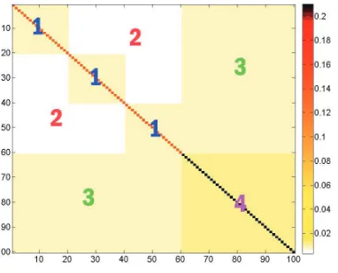
and off-diagonal entries equal toα_∈[0,1). For the Frobenius norm and nuclear norm bounds, we construct anm_×mblock diagonal matrixAwhich haskdiagonal blocks, each of which ism_k _×m_k in

size and constructed in the same way asB. For the lower bounds on_maxkA−A˜kξ

i,j|ai j|,αis set to be constant; for the bounds on kA−A˜kξ

kA−Akkξ,αis set to beα→1. The detailed proof of Theorem 12 is deferred to Appendix C.

Theorem 12 (Lower Error Bounds of the Nystr¨om Methods) Assume we are given an SPSD

ma-trixA_∈Rm×mand a target rank k. LetAkdenote the best rank-k approximation toA. LetA˜ denote

either the rank-c approximation to Aconstructed by the standard Nyström method in (1), or the approximation constructed by the ensemble Nyström method in (2) with t non-overlapping samples, each of which contains c columns ofA. Then there exists an SPSD matrix such that for any sampling strategy the approximation errors of the conventional Nyström methods, that is,_kA₋A˜_k_ξ,(ξ=2, F, or “_∗”), are lower bounded by some factors which are shown in Table 3.

Remark 13 The lower bounds in Table 3 (or Table 2) show the conventional Nystr¨om methods can

be sometimes very ineffective. The spectral norm and Frobenius norm bounds even depend on m, so such bounds are not constant-factor bounds. Notice that the lower error bounds do not meet ifW†

is replaced byC†A(C†)T_{, so our modified Nystr¨om method is not limited by such lower bounds.}

4.5 Discussions of the Expected Relative-Error Bounds

The upper error bounds established in this paper all hold in expectation. Now we show that the expected error bounds immediately extend to w.h.p. bounds using Markov’s inequality. Let the random variableX =_kA₋A˜_kF/kA−AkkF denote the error ratio, where

˜

A=CUR or CUCT.

Then we haveE(X)_≤1+εby the preceding theorems. By applying Markov’s inequality we have that

P X>1+sε < E(X)

1+sε <

1+ε

1+sε,

wheresis an arbitrary constant greater than 1. Repeating the sampling procedure fort times and lettingX(i)correspond to the error ratio of thei-th sample, we obtain an upper bound on the failure probability:

Pmin

i {X(i)}>1+sε

= PX(i)>1+sε∀i=1,···,t

< 1+ε

1+sε t

, δ, (4)

which decays exponentially witht. Therefore, by repeating the sampling procedure multiple times and choosing the best sample, our CUR and Nystr¨om algorithms are also guaranteed with w.h.p. relative-error bounds. It follows directly from (4) that, by repeating the sampling procedure for

t _≥ 1+ε (s₋1)εlog

₁

δ

times, the inequality

(15)

holds with probability at least 1₋δ.

For instance, we lets=1+log(1/δ), then by repeating the sampling procedure fort_≥1+1/ε

times, the inequality

kA₋A˜_kF ≤

1+ε+εlog(1/δ)_kA₋AkkF

For another instance, we let s =2, then by repeating the sampling procedure for t _≥(1+ 1/ε)log(1/δ)times, the inequality

kA₋A˜_kF ≤ (1+2ε)kA−AkkF

5. Empirical Analysis

In Section 5.1 we empirical evaluate our CUR algorithms in comparison with the algorithms in-troduced in Section 3.3. In Section 5.2 we conduct empirical comparisons between the standard Nystr¨om and our modified Nystr¨om, and comparisons among three sampling algorithms. We report the approximation error incurred by each algorithm on each data set. The error ratio is defined by

Error Ratio = kA−A˜kF

kA₋AkkF

,

where Ã=CUR for the CUR matrix decomposition, Ã=CW†CT for the standard Nyström method, and Ã=C C†A(C†)T_CT _{for the modified Nyström method.}

We conduct experiments on a workstation with two Intel Xeon 2.40GHz CPUs, 24GB RAM, and 64bit Windows Server 2008 system. We implement the algorithms in MATLAB R2011b, and use the MATLAB function ‘svds’ for truncated SVD. To compare the running time, all the compu-tations are carried out in a single thread by setting ‘maxNumCompThreads(1)’ in MATLAB.

5.1 Comparison among the CUR Algorithms

In this section we empirically compare our adaptive sampling based CUR algorithm (Algorithm 2) with the subspace sampling algorithm of Drineas et al. (2008) and the deterministic sparse column-row approximation (SCRA) algorithm of Stewart (1999). For SCRA, we use the MATLAB code released by Stewart (1999). As for the subspace sampling algorithm, we compute the leverages scores exactly via the truncated SVD. Although the fast approximation to leverage scores (Drineas et al., 2012) can significantly speedup subspace sampling, we do not use it because the approxima-tion has no theoretical guarantee when applied to subspace sampling.

Data Set Type Size #Nonzero Entries Source

Enron Emails text 39,861×28,102 3,710,420 Bag-of-words, UCI Dexter text 20,000×2,600 248,616 Guyon et al. (2004) Farm Ads text 54,877×4,143 821,284 Mesterharm and Pazzani (2011)

Gisette handwritten digit 13,500_×5,000 8,770,559 Guyon et al. (2004)

(16)

3 5 7 9 11 13 15 17 19 21 23 25 0 500 1000 1500 2000 2500 3000 3500 4000 T ime (s) a Elapsed Time Adaptive Sampling Subspace Sampling Deterministic

3 4 5 6 7 8 9 10 11 12 13 14 15 16 17 18 19 20 0 0.5 1 1.5 2 2.5 3 3.5

4x 10

4 T ime (s) a Elapsed Time Adaptive Sampling Subspace Sampling Deterministic

3 5 7 9 11 13 15 17 19 21 23 25 0.7 0.8 0.9 1 1.1 1.2 1.3 1.4 Erro r R a ti o a Approximation Error Adaptive Sampling Subspace Sampling Deterministic

(a)k=10,c=ak, andr=ac.

3 4 5 6 7 8 9 10 11 12 13 14 15 16 17 18 19 20 0.4 0.6 0.8 1 1.2 1.4 1.6 1.8 2 Erro r R a ti o a Approximation Error Adaptive Sampling Subspace Sampling Deterministic

(b)k=50,c=ak, andr=ac.

Figure 1: Results of the CUR algorithms on the Enron data set.

3 5 7 9 11 13 15 17 19 21 23 25 0 200 400 600 800 1000 1200 1400 1600 1800 2000 T ime (s) a Elapsed Time Adaptive Sampling Subspace Sampling Deterministic

3 4 5 6 7 8 9 10 11 12 13 14 15 16 17 18 19 20 0 500 1000 1500 2000 2500 3000 T ime (s) a Elapsed Time Adaptive Sampling Subspace Sampling Deterministic

3 5 7 9 11 13 15 17 19 21 23 25 0.9 0.95 1 1.05 1.1 1.15 Erro r R a ti o a Approximation Error Adaptive Sampling Subspace Sampling Deterministic

3 4 5 6 7 8 9 10 11 12 13 14 15 16 17 18 19 20 0.7 0.8 0.9 1 1.1 1.2 1.3 1.4 Erro r R a ti o a Approximation Error Adaptive Sampling Subspace Sampling Deterministic

(17)

3 5 7 9 11 13 15 17 19 21 23 25 0 500 1000 1500 2000 2500 3000 T ime (s) a Elapsed Time Adaptive Sampling Subspace Sampling Deterministic

3 4 5 6 7 8 9 10 11 12 13 14 15 16 17 18 19 20 0 1000 2000 3000 4000 5000 6000 7000 8000 T ime (s) a Elapsed Time Adaptive Sampling Subspace Sampling Deterministic

3 5 7 9 11 13 15 17 19 21 23 25 0.75 0.8 0.85 0.9 0.95 1 1.05 1.1 1.15 1.2 Erro r R a ti o a Approximation Error Adaptive Sampling Subspace Sampling Deterministic

3 4 5 6 7 8 9 10 11 12 13 14 15 16 17 18 19 20 0.5 0.6 0.7 0.8 0.9 1 1.1 Erro r R a ti o a Approximation Error Adaptive Sampling Subspace Sampling Deterministic

Figure 3: Results of the CUR algorithms on the Farm Ads data set.

3 5 7 9 11 13 15 17 19 21 23 25 0 500 1000 1500 2000 2500 3000 3500 4000 4500 T ime (s) a Elapsed Time Adaptive Sampling Subspace Sampling Deterministic

3 4 5 6 7 8 9 10 11 12 13 14 0 500 1000 1500 2000 2500 3000 3500 T ime (s) a Elapsed Time Adaptive Sampling Subspace Sampling Deterministic

3 5 7 9 11 13 15 17 19 21 23 25 0.85 0.9 0.95 1 1.05 1.1 1.15 1.2 1.25 Erro r R a ti o a Approximation Error Adaptive Sampling Subspace Sampling Deterministic

3 4 5 6 7 8 9 10 11 12 13 14 0.8 0.85 0.9 0.95 1 1.05 1.1 1.15 1.2 1.25 Erro r R a ti o a Approximation Error Adaptive Sampling Subspace Sampling Deterministic

(18)

We conduct experiments on four UCI data sets (Frank and Asuncion, 2010) which are sum-marized in Table 4. Each data set is represented as a data matrix, upon which we apply the CUR algorithms. According to our analysis, the target rankk should be far less thanmandn, and the column numberc and row numberrshould be strictly greater thank. For each data set and each algorithm, we setk=10 or 50, andc=ak,r=ac, wherearanges in each set of experiments. We repeat each of the two randomized algorithms 10 times, and report the minimum error ratio and the total elapsed time of the 10 rounds. We depict the error ratios and the elapsed time of the three CUR matrix decomposition algorithms in Figures 1, 2, 3, and 4.

We can see from Figures 1, 2, 3, and 4 that our adaptive sampling based CUR algorithm has much lower approximation error than the subspace sampling algorithm in all cases. Our adaptive sampling based algorithm is better than the deterministic SCRA on the Farm Ads data set and the Gisette data set, worse than SCRA on the Enron data set, and comparable to SCRA on the Dexter data set. In addition, the experimental results match our theoretical analysis in Section 4 very well. The empirical results all obey the theoretical relative-error upper bound

kA₋CUR_kF

kA₋AkkF ≤

1+2k

c 1+o(1)

= 1+2

a 1+o(1)

.

As for the running time, the subspace sampling algorithm and our adaptive sampling based algorithm are much more efficient than SCRA, especially when c andr are large. Our adaptive sampling based algorithm is comparable to the subspace sampling algorithm when c and r are small; however, our algorithm becomes less efficient when c andr are large. This is due to the following reasons. First, the computational cost of the subspace sampling algorithm is dominated by the truncated SVD ofA, which is determined by the target rankkand the size and sparsity of the data matrix. However, the cost of our algorithm grows withcandr. Thus, our algorithm becomes less efficient whenc andr are large. Second, the truncated SVD operation in MATLAB, that is, the ‘svds’ function, gains from sparsity, but our algorithm does not. The four data sets are all very sparse, so the subspace sampling algorithm has advantages. Third, the truncated SVD functions are very well implemented by MATLAB (not in MATLAB language but in Fortran/C). In contrast, our algorithm is implemented in MATLAB language, which is usually less efficient than Fortran/C.

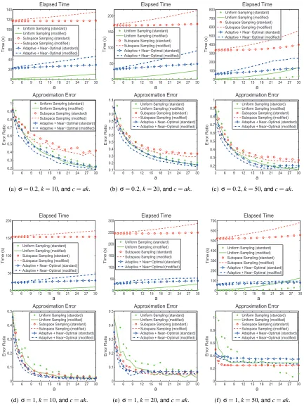
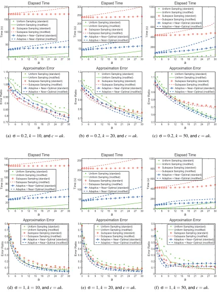
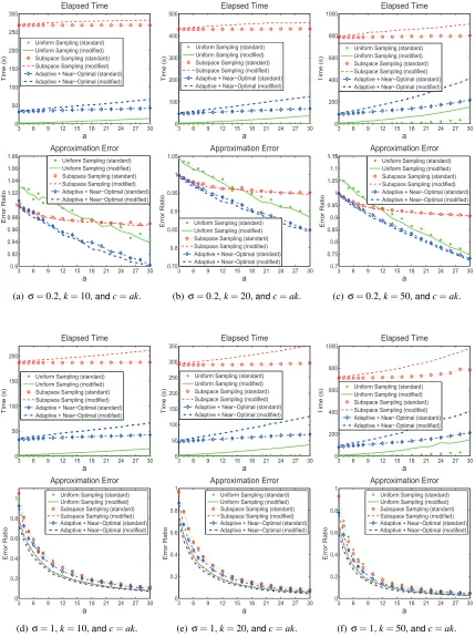
5.2 Comparison among the Nystr¨om Algorithms

In this section we empirically compare our adaptive sampling algorithm (in Theorem 10) with some other sampling algorithms including the subspace sampling of Drineas et al. (2008) and the uniform sampling, both without replacement. We also conduct comparison between the standard Nystr¨om and our modified Nystr¨om, both use the three sampling algorithms to select columns.

We test the algorithms on three data sets which are summarized in Table 5. The experiment setting follows Gittens and Mahoney (2013). For each data set we generate a radial basis function (RBF) kernel matrixAwhich is defined by

ai j=exp

−kxi−xjk 2 2

2σ2

,

wherexiandxj are data instances andσis a scale parameter. Notice that the RBF kernel is dense

(19)

Data Set #Instances #Attributes Source

Abalone 4,177 8 UCI (Frank and Asuncion, 2010) Wine Quality 4,898 12 UCI (Cortez et al., 2009)

Letters 5,000 16 Statlog (Michie et al., 1994)

kA₋AkkF/kAkF mkstd ℓ[k]

k=10 k=20 k=50 k=10 k=20 k=50

Abalone (σ=0.2) 0.4689 0.3144 0.1812 0.8194 0.6717 0.4894 Abalone (σ=1.0) 0.0387 0.0122 0.0023 0.5879 0.8415 1.3830 Wine Quality (σ=0.2) 0.8463 0.7930 0.7086 1.8703 1.6490 1.3715 Wine Quality (σ=1.0) 0.0504 0.0245 0.0084 0.3052 0.5124 0.8067 Letters (σ=0.2) 0.9546 0.9324 0.8877 5.4929 3.9346 2.6210 Letters (σ=1.0) 0.1254 0.0735 0.0319 0.2481 0.2938 0.3833

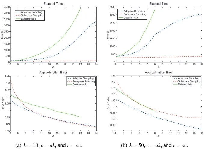
Table 5: A summary of the data sets for the Nystr¨om approximation. In the second tabularstd ℓ[k] denotes the standard deviation of the statistical leverage scores of Arelative to the best rank-kapproximation toA. We use the normalization factor m_k because m_kmean ℓ[k]₌_1.

ofσandkin the following two paragraphs. We run each algorithm for 10 times, and report the the minimum error ratio as well as the total elapsed time of the 10 repeats. The results are shown in Figures 5, 6, and 7.

Table 5 provides useful implications on choosing the target rankk. In Table 5, kA−AkkF

kAkF denotes ratio that is not captured by the best rank-k approximation to the RBF kernel, and the parameter

σhas an influence on the ratio _kA₋AkkF/kAkF. Whenσ is large, the RBF kernel can be well

approximated by a low-rank matrix, which implies that (i) a smallksuffices whenσis large, and (ii) kshould be set large whenσis small. So the settings (σ=1,k=10) and (σ=0.2,k=50) are more reasonable than the rest. Let us take the RBF kernel in the Abalone data set as an example. When

σ=1, the rank-10 approximation well captures the kernel, so kcan be safely set as small as 10; whenσ=0.2, the target rankkshould be set large, say larger than 50, otherwise the approximation is rough.

The standard deviation of the leverage scores reflects whether the advanced importance sam-pling techniques such as the subspace samsam-pling and adaptive samsam-pling are useful. Figures 5, 6, and 7 show that the advantage of the subspace sampling and adaptive sampling over the uniform sampling is significant whenever the standard deviation of the leverage scores is large (see Table 5), and vise versa. Actually, as reflected in Table 5, the parameterσinfluences the homogeneity/heterogeneity of the leverage scores. Usually, whenσis small, the leverage scores become heterogeneous, and the effect of choosing “good” columns is significant.

(20)

3 6 9 12 15 18 21 24 27 30 0 20 40 60 80 100 120 140 T ime (s) a Elapsed Time

Uniform Sampling (standard) Uniform Sampling (modified) Subspace Sampling (standard) Subspace Sampling (modified) Adaptive + Near−Optimal (standard) Adaptive + Near−Optimal (modified)

3 6 9 12 15 18 21 24 27 30 0 50 100 150 200 T ime (s) a Elapsed Time

3 6 9 12 15 18 21 24 27 30 0 100 200 300 400 500 600 700 800 T ime (s) a Elapsed Time

3 6 9 12 15 18 21 24 27 30 0.2 0.3 0.4 0.5 0.6 0.7 0.8 0.9 1 Erro r R a ti o a Approximation Error

(a) σ=0.2,k=10, andc=ak.

3 6 9 12 15 18 21 24 27 30 0.1 0.2 0.3 0.4 0.5 0.6 0.7 0.8 0.9 1 1.1 1.1 Erro r R a ti o a Approximation Error

(b)σ=0.2,k=20, andc=ak.

3 6 9 12 15 18 21 24 27 30 0.2 0.3 0.4 0.5 0.6 0.7 0.8 0.9 1 Erro r R a ti o a Approximation Error

(c)σ=0.2,k=50, andc=ak.

3 6 9 12 15 18 21 24 27 30 0 50 100 150 200 250 300 T ime (s) a Elapsed Time

3 6 9 12 15 18 21 24 27 30 0 0.1 0.2 0.3 0.4 0.5 Erro r R a ti o a Approximation Error

(d)σ=1,k=10, andc=ak.

3 6 9 12 15 18 21 24 27 30 0 0.1 0.2 0.3 0.4 0.5 Erro r R a ti o a Approximation Error

(e) σ=1,k=20, andc=ak.

3 6 9 12 15 18 21 24 27 30 0 0.2 0.4 0.6 0.8 1 Erro r R a ti o a Approximation Error

(f) σ=1,k=50, andc=ak.

(21)

3 6 9 12 15 18 21 24 27 30 0 200 400 600 800 1000 T ime (s) a Elapsed Time

3 6 9 12 15 18 21 24 27 30 0.75 0.8 0.85 0.9 0.95 1 1.05 1.1 1.15 Erro r R a ti o a Approximation Error

(a) σ=0.2,k=10, andc=ak.

3 6 9 12 15 18 21 24 27 30 0.7 0.8 0.9 1 1.1 1.2 Erro r R a ti o a Approximation Error

(b)σ=0.2,k=20, andc=ak.

3 6 9 12 15 18 21 24 27 30 0.5 0.6 0.7 0.8 0.9 1 1.1 Erro r R a ti o a Approximation Error

(c)σ=0.2,k=50, andc=ak.

3 6 9 12 15 18 21 24 27 30 0 20 40 60 80 100 120 140 160 T ime (s) a Elapsed Time

3 6 9 12 15 18 21 24 27 30 0 0.1 0.2 0.3 0.4 0.5 0.6 0.7 0.8 Erro r R a ti o a Approximation Error

(22)

3 6 9 12 15 18 21 24 27 30 0.9 0.92 0.94 0.96 0.98 1 1.02 1.04 1.06 1.08 Erro r R a ti o a Approximation Error

(a) σ=0.2,k=10, andc=ak.

3 6 9 12 15 18 21 24 27 30 0.75 0.8 0.85 0.9 0.95 1 1.05 Erro r R a ti o a Approximation Error

(b)σ=0.2,k=20, andc=ak.

3 6 9 12 15 18 21 24 27 30 0.7 0.75 0.8 0.85 0.9 0.95 1 1.05 1.1 1.15 1.15 Erro r R a ti o a Approximation Error

(c)σ=0.2,k=50, andc=ak.

(23)

Theorem 10; that is,

kA₋CUCT_kF

kA₋AkkF ≤

1+

r

2k

c 1+o(1)

= 1+

r

2

a 1+o(1)

.

As for the running time, our adaptive sampling algorithm is more efficient than the subspace sam-pling algorithm. This is partly because the RBF kernel matrix is dense, and hence the subspace sampling algorithm costs

O

_(m2_k)_{time to compute the truncated SVD.}

Furthermore, the experimental results show that usingU=C†A(C†)T_{as the intersection matrix}

(denoted by “modified” in the figures) always leads to much lower error than usingU=W†_(denoted

by “standard”). However, our modified Nyström method costs more time to compute the intersection matrix than the standard Nyström method costs. Recall that the standard Nyström costs

O

_(c3₎_time

to computeU=W†_{and that the modified Nystr¨om costs}

_O

_(mc2_{) +}_T

Multiply(m2c)time to compute

U=C†A(C†)T_{. So the users should make a trade-off between time and accuracy and decide whether}

it is worthwhile to sacrifice extra computational overhead for the improvement in accuracy by using the modified Nystr¨om method.

6. Conclusion

In this paper we have built a novel and more general relative-error bound for the adaptive sampling algorithm. Accordingly, we have devised novel CUR matrix decomposition and Nystr¨om approxi-mation algorithms which demonstrate significant improvement over the classical counterparts. Our relative-error CUR algorithm requires onlyc=2kε−1₍₁₊_o(1))_{columns and}_r₌_c_ε−1₍₁₊_ε₎_rows

selected from the original matrix. To achieve relative-error bound, the best previous algorithm— the subspace sampling algorithm—requiresc=

O

_(k_ε−2_logk)_{columns and}_r₌

_O

_(c_ε₋2_log_c)_rows.

Our modified Nyström method is different from the conventional Nyström methods in that it uses a different intersection matrix. We have shown that our adaptive sampling algorithm for the modified Nyström achieves relative-error upper bound by sampling onlyc=2kε−2_(1+o(1))_{columns, which}

even beats the lower error bounds of the standard Nyström and the ensemble Nyström. Our proposed CUR and Nyström algorithms are scalable because they need only to maintain a small fraction of columns or rows in RAM, and their time complexities are low provided that matrix multiplication can be highly efficiently executed. Finally, the empirical comparison has also demonstrated the effectiveness and efficiency of our algorithms.

Acknowledgments

This work has been supported in part by the Natural Science Foundations of China (No. 61070239) and the Scholarship Award for Excellent Doctoral Student granted by Chinese Ministry of Educa-tion.

Appendix A. The Dual Set Sparsification Algorithm

(24)

Algorithm 3Deterministic Dual Set Spectral-Frobenius Sparsification Algorithm.

1: Input:U₌_{_x_i_}n

i=1⊂Rl, (l<n);V ={vi}ni=1⊂Rk, with∑ n

i=1vivTi =Ik(k<n);k<r<n; 2: Initialize: s0=0,A0=0;

3: Computekxik22fori=1,···,n, and then computeδU=∑

n i=1kxik22 1₋√k/r ; 4: forτ=0 tor₋1do

5: Compute the eigenvalue decomposition ofAτ;

6: Find any index jin{1,···,n_}and compute a weightt>0 such that

δ−1

U kxjk22 ≤ t−1 ≤

vT_jAτ−(Lτ+1)Ik

−2

vj

φ(Lτ+1,Aτ)−φ(Lτ,Aτ) −

vT_jAτ−(Lτ+1)Ik

−1

vj;

where

φ(L,A) =

k

∑

i=1

λi(A)−L

₋1

, Lτ=τ−

√

rk;

7: Update the j-th component ofsτandAτ: sτ+1[j] =sτ[j] +t, Aτ+1=Aτ+tvjvTj;

8: end for

9: return s=1−

√

k/r r sr.

algorithm in Algorithm 3 and its bounds in Lemma 14, and we also analyze the time complexity using our defined notation.

Lemma 14 (Dual Set Spectral-Frobenius Sparsification) Let

U

₌_{_x₁_,_···_,_x_n_{} ⊂}_Rl_(l_<_n)

con-tain the columns of an arbitrary matrixX_∈Rl×n_{. Let}

_V

₌_{_v

1,···,vn} ⊂Rk (k<n)be a

decom-positions of the identity, that is, ∑ni=1vivTi =Ik. Given an integer r with k<r <n, Algorithm 3

deterministically computes a set of weights si≥0 (i=1,···,n) at most r of which are non-zero,

such that

λk

n

∑

i=1

sivivTi

≥1₋

r

k r

2

and tr

n

∑

i=1

sixixTi

≤ kX_k2_F.

The weights sican be computed deterministically in

O

rnk2

+TMultiply nl

time.

Here we mention some implementation issues of Algorithm 3 which were not described in detail by Boutsidis et al. (2011). In each iteration the algorithm performs once eigenvalue decomposition:

Aτ=WΛWT. HereAτis guaranteed to be SPSD in each iteration. Since

Aτ−αIk

q

= WDiag(λ1−α)q,···,(λk−α)q

WT,

(Aτ−(Lτ+1)Ik)qcan be efficiently computed based on the eigenvalue decomposition ofAτ. With

the eigenvalues at hand,φ(L,Aτ)can also be computed directly.

The algorithm runs inriterations. In each iteration, the eigenvalue decomposition ofAτrequires