From Predictive Methods to Missing Data Imputation:
An Optimization Approach
Dimitris Bertsimas [email protected]
Colin Pawlowski [email protected]
Ying Daisy Zhuo [email protected]
Sloan School of Management and Operations Research Center Massachusetts Institute of Technology
Cambridge, MA 02139
Editor:Francis Bach
Abstract
Missing data is a common problem in real-world settings and for this reason has attracted significant attention in the statistical literature. We propose a flexible framework based on formal optimization to impute missing data with mixed continuous and categorical variables. This framework can readily incorporate various predictive models including K-nearest neighbors, support vector machines, and decision tree based methods, and can be adapted for multiple imputation. We derive fast first-order methods that obtain high quality solutions in seconds following a general imputation algorithmopt.imputepresented in this paper. We demonstrate that our proposed method improves out-of-sample accuracy in large-scale computational experiments across a sample of 84 data sets taken from the UCI Machine Learning Repository. In all scenarios of missing at random mechanisms and various missing percentages, opt.impute produces the best overall imputation in most data sets benchmarked against five other methods: mean impute, K-nearest neighbors, iterative knn, Bayesian PCA, and predictive-mean matching, with an average reduction in mean absolute error of 8.3% against the best cross-validated benchmark method. Moreover, opt.impute leads to improved out-of-sample performance of learning algorithms trained using the imputed data, demonstrated by computational experiments on 10 downstream tasks. For models trained using opt.impute single imputations with 50% data missing, the average out-of-sampleR2is 0.339 in the regression tasks and the average out-of-sample
accuracy is 86.1% in the classification tasks, compared to 0.315 and 84.4% for the best cross-validated benchmark method. In the multiple imputation setting, downstream models trained usingopt.imputeobtain a statistically significant improvement over models trained using multivariate imputation by chained equations (mice) in 8/10 missing data scenarios considered.
Keywords: missing data imputation,K-NN, SVM, optimal decision trees
1. Introduction
The missing data problem is arguably the most common issue encountered by machine learning practitioners when analyzing real-world data. In many applications ranging from gene expression in computational biology to survey responses in social sciences, missing data is present to various degrees. As many statistical models and machine learning algorithms rely on complete data sets, it is key to handle the missing data appropriately.
c
Method Name Category Software Reference
Mean impute (mean) Mean Little and Rubin (1987)
Expectation-Maximization (EM) EM Dempster et al. (1977) EM with Mixture of Gaussians and Multinomials EM Ghahramani and Jordan (1994) EM with Bootstrapping EM Amelia II Honaker et al. (2011)
K-Nearest Neighbors (knn) K-NN impute Troyanskaya et al. (2001) SequentialK-Nearest Neighbors K-NN Kim et al. (2004)
IterativeK-Nearest Neighbors K-NN Caruana (2001); Br´as and Menezes (2007)
Support Vector Regression SVR Wang et al. (2006)
Predictive-Mean Matching (pmm) LS MICE Buuren and Groothuis-Oudshoorn (2011)
Least Squares LS Bø et al. (2004)
Sequential Regression Multivariate Imputation LS Raghunathan et al. (2001)
Local-Least Squares LS Kim et al. (2005)
Sequential Local-Least Squares LS Zhang et al. (2008)
Iterative Local-Least Squares LS Cai et al. (2006)
Sequential Regression Trees Tree MICE Burgette and Reiter (2010) Sequential Random Forest Tree missForest Stekhoven and B¨uhlmann (2012) Singular Value Decomposition SVD Troyanskaya et al. (2001) Bayesian Principal Component Analysis SVD pcaMethods Oba et al. (2003); Mohamed et al. (2009) Factor Analysis Model for Mixed Data FA Khan et al. (2010)
Table 1: List of Imputation Methods
In some cases, simple approaches may suffice to handle missing data. For example, complete-case analysis uses only the data that is fully known and omits all observations with missing values to conduct statistical analysis. This works well if only a few observations contain missing values, and when the data is missing completely at random, complete-case analysis does not lead to biased results (Little and Rubin, 1987). Alternately, some machine learning algorithms naturally account for missing data, and there is no need for preprocessing. For instance, CART and K-means have been adapted for problems with missing data (Breiman et al., 1984; Wagstaff, 2004).
In many other situations, missing values need to be imputed prior to running statistical analyses on the complete data set. The benefit of the latter approach is that once a set (or multiple sets) of complete data has been generated, practitioners can easily apply their own learning algorithms to the imputed data set. We focus on methods for missing data imputation in this paper.
Concretely, assume that we are given data X = {x1, . . . ,xn} with missing entries xid,(i, d)∈ M. The objective is to impute the values of the missing data that resemble the
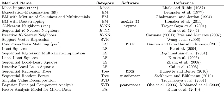
underlying complete data as closely as possible. This way, when one conducts statistical inference or pattern recognition using machine learning methods on the imputed data, the results should be similar to those obtained if full data were given. We outline some of the state-of-the-art methods for imputation in Table 1 and describe them briefly below. Part of the list is adapted from a review paper by Liew et al. (2011).
1.1 Related Work
The simplest method is mean impute, in which each missing valuexidis imputed as the mean
Joint modeling asserts some joint distribution on the entire data set. It assumes a para-metric density function (e.g., multivariate normal) on the data given model parameters. In practice, model parameters are typically estimated using an Expectation-Maximization (EM) approach. It finds a solution (often non-optimal) of missing values and model pa-rameters to maximize the likelihood function. Many software tools such as the R package Amelia 2implement the EM method with bootstrapping, assuming that the data is drawn from a multivariate normal distribution (Honaker et al., 2011). Joint modeling provides useful theoretical properties but lacks the flexibility for processing data types seen in many real applications (Van Buuren, 2007). For example, when the data includes continuous and categorical variable types, standard multivariate density functions often fail at modeling the complexity of mixed data types. However, under the assumption that the categorical variables are independent, we can use mixture models of Gaussians and Multinomials for imputation (Ghahramani and Jordan, 1994).
In contrast to joint modeling, fully conditional specification is a more flexible alterna-tive where one specifies the conditional model for each variable; it is especially useful in mixed data types (Van Buuren, 2007). To generalize to multivariate settings, a chained equation process — initializing using random sampling and conducting univariate imputa-tions sequentially until convergence — is typically used (Buuren and Groothuis-Oudshoorn, 2011). Each iteration is a Gibbs sampler that draws from the conditional distribution on the imputed values.
A simple example of conditional specification is based on regression. Least-Squares (LS) imputation constructs single univariate regressions, regressing features with missing values on all of the other dimensions in the data. Each missing value xid is then imputed as the
weighted average of these regression predictions (Bø et al., 2004; Raghunathan et al., 2001). Alternatively, in the Predictive-Mean Matching method (pmm), imputations are random samples drawn from a set of observed values close to regression predictions (Buuren and Groothuis-Oudshoorn, 2011). Imputation methods that use Support Vector Regression in place of LS for the regression step have also been explored (Wang et al., 2006).
When there is non-linear relationship between the variables, linear regression based imputation may perform poorly. Burgette and Reiter (2010) propose using Classification and Regression Trees (CART) as the conditional model for imputation. Extensions to random forests have also shown promising results (Stekhoven and B¨uhlmann, 2012). These decision tree based imputation methods are non-parametric approaches that do not rely upon distributional assumptions on the data.
One of the most commonly used non-parametric approaches isK-Nearest Neighbors (K -NN) based imputation. This method imputes each missing entryxidas the mean of thedth
dimension of theK-nearest neighbors that have observed values in dimensiond(Troyanskaya et al., 2001). Some extensions ofK-NN include sequentialK-NN, which starts by imputing missing values from observations with the fewest missing dimensions and continues imputing the next unknown entries reusing the previously imputed values (Kim et al., 2004). Iterative
xi (Kim et al., 2005). Sequential and iterative variations of Local-Least Squares resemble
theirK-NN imputation counterparts (Zhang et al., 2008; Cai et al., 2006).
Low dimensional representation-based imputation assumes that the data represents a noisy observation of a linear combination of a small set of principal components or factor variables. In the basic method, singular value decomposition (SVD) is used on the entire data set to determine the principal eigenvectors. The missing values are imputed as a linear combination of these eigenvectors. This process is iteratively repeated until conver-gence (Troyanskaya et al., 2001; Mazumder et al., 2010). Bayesian Principal Component Analysis is similar to SVD imputation but extends the method to incorporate information from a prior distribution on the model parameters (Oba et al., 2003; Mohamed et al., 2009). Some recent development of a variant of the EM algorithm for factor analysis also provides a missing data imputation method for mixed data (Khan et al., 2010).
Thus far, we have only discussed methods for single imputation which generate one set of completed data that will be used for further statistical analyses. Multiple imputation, on the other hand, imputes multiple times (each set is possibly different), runs the statistical analyses on each, and pools the results (Little and Rubin, 1987). Such method is able to capture the variability in the missing data and therefore generate potentially more accurate estimates to the larger statistical problem. However, multiple imputation methods are slower and require pooling results, which may not be appropriate for certain applications.
Within the multiple imputation framework, the procedure for generating multiple es-timates of missing values varies. Multivariate imputation by chained equations (mice), a popular multiple imputation method, generates estimates using: predictive mean match-ing, Bayesian linear regression, logistic regression, and others (Buuren and Groothuis-Oudshoorn, 2011). In all cases, the method initializes using random sampling and conducts univariate imputations sequentially until convergence. Each iteration is a Gibbs sampler that draws from the conditional distribution on the imputed values.
Because of its importance, missing data imputation remains an active research area. Although there are numerous methods, many of them have serious shortcomings. Joint modeling methods are not as effective when data sets violate normality assumptions, and a na¨ıve implementation often crashes during the computation of a singular covariance ma-trix (Honaker et al., 2011). Some conditional specification methods such as pmmare practi-cally reliable, but lack theoretical foundation and have no explicit formulation as an opti-mization problem. This stands in stark contrast to other areas of machine learning, where statistical models and optimization problems are deeply intertwined.
1.2 Contributions
We summarize our contributions in this paper below:
1. We pose the missing data problem under a general optimization framework. The framework produces an optimization problem with a predictive model-based cost func-tion that explicitly handles both continuous and categorical variables and can be used to generate multiple imputations. We present three cost functions derived from K -nearest neighbors, support vector machines, and optimal decision tree models. This optimization perspective provides fresh insight into the classical missing data problem and leads to new algorithms for more accurate data imputation.
2. For each imputation model, we derive first-order methods to find high-quality solutions to the missing data problem following a general imputation algorithmopt.impute pre-sented in this paper. These methods easily scale to data sets with n in the 100,000s and p in the 1,000s on a standard desktop computer and converge within a few it-erations. In addition, the first-order methods are robust and reliable for arbitrary missing patterns and mixed data types.
3. We evaluate the methods in computational experiments using 84 real-world data sets taken from the UCI Machine Learning Repository. Benchmarked against exist-ing imputation methods includexist-ing mean impute, K-nearest neighbors, iterative knn, Bayesian PCA, and predictive-mean matching,opt.imputeproduces the best overall imputation in more than 75.8% of all data sets, and results in an average reduction in mean absolute error of 8.3% against the best cross-validated benchmark method.
4. We demonstrate that the improved data imputations generated by opt.impute give rise to improved performance on 10 downstream classification and regression tasks. With 50% of missing data, classification models trained on data imputed viaopt.impute have an average testing accuracy of 86.1% compared to 84.4% for the best cross-validated benchmark method. In addition, regression models trained on data imputed via opt.impute have an average out-of-sample R2 value of 0.339 compared to 0.315 for the best cross-validated benchmark method. Finally, downstream models trained on multiple imputations produced by opt.impute significantly outperform multiple imputations produced bymicein 3/5 missing data scenarios for classification and 5/5 scenarios for regression.
2. Methods for Optimal Imputation
In this section, we pose the missing data problem as an optimization problem in which we optimize the missing values in all data points and dimensions simultaneously. We introduce a general imputation framework on mixed data (continuous and categorical) based upon first-order methods applied to this problem. Within this framework, we use K-nearest neighbors, SVM, and decision tree based imputation as examples to define three specific optimization problems. For each problem, we present two first-order methods used to find high-quality solutions: block coordinate descent (BCD) and coordinate descent (CD).
Let X = {xi}ni=1 be the data set given with p variables. Without loss of generality, we assume each data vector xi contains continuous variables indexed by d∈ {1,2, . . . , p0} and categorical variables indexed by d ∈ {p0 + 1, . . . , p0 +p1} with p0 +p1 = p. As a pre-processing step, we transform all continuous variables to have unit standard deviation. We leave all categorical variables unchanged, and assume the dth categorical variable d∈ {p0 + 1, . . . , p0 +p1} takes values among kd classes. Note that if all data is continuous p0 = 0, while if all data is categorical p1 = 0. The missing and known values are specified by the following sets:
M0 ={(i, d) : entry xid is missing, 1≤d≤p0}, N0 ={(i, d) : entry xid is known, 1≤d≤p0},
M1 ={(i, d) : entry xid is missing, p0+ 1≤d≤p0+p1}, N1 ={(i, d) : entry xid is known, p0+ 1≤d≤p0+p1}.
We also refer to the full missing pattern asM:=M0∪ M1. LetW ∈Rn×p0 be the matrix
of imputed continuous values, wherewid is the imputed value for entryxid,d∈ {1, . . . , p0}. Similarly, letV∈ {1, . . . , k1}×. . .×{1, . . . , kp1}be the matrix of imputed categorical values,
wherevid is the imputed value for entry xid,d∈ {p0+ 1, . . . , p0+p1}. We refer to the full imputation for observation xi as (wi,vi) in the following sections.
2.1 General Problem Formulation
As the task is to impute the missing values, for each model the key decision variables are the imputed values{wid: (i, d)∈ M0}and {vid: (i, d)∈ M1}. We also introduce auxiliary decision variables as well; denote these as U. For instance, in a K-NN based approach, indicator variables zij,1 ≤i, j ≤n are introduced to identify the neighbor assignment for
each pair of points xi, xj. For a given set of imputed values and a given model, there
is a cost function c(·) associated with it. Our goal is to solve the following optimization problem:
min c(U,W,V;X)
s.t. wid=xid (i, d)∈ N0,
vid=xid (i, d)∈ N1, (U,W,V)∈ U,
(1)
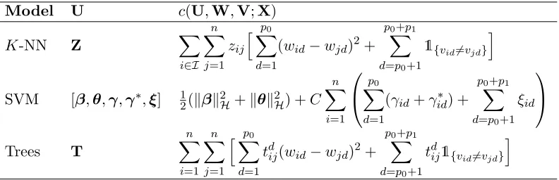
point has exactly K neighbors and the assignment variables are binary. We list the aux-iliary variables and cost functions corresponding to each of the imputation modelsK-NN, SVM, and trees in Table 2. Note that the cost function can be different for continuous and categorical variables. We can introduce a parameter that controls the relative contri-bution to the cost between the continuous and categorical variables, or scale continuous variables appropriately. For the remainder of the paper the latter is assumed for simplicity of notation.
Model U c(U,W,V;X)
K-NN Z X
i∈I
n
X
j=1
zij
hXp0
d=1
(wid−wjd)2+ p0+p1
X
d=p0+1
1{vid6=vjd}
i
SVM [β,θ,γ,γ∗,ξ] 12(kβk2
H+kθk2H) +C
n
X
i=1
p0 X
d=1
(γid+γid∗) + p0+p1
X
d=p0+1 ξid
Trees T
n
X
i=1
n
X
j=1
hXp0
d=1
tdij(wid−wjd)2+ p0+p1
X
d=p0+1
tdij1{vid6=vjd}
i
Table 2: Variables and cost functions for each imputation model. Variables for K-NN, SVM, and trees are defined in Sections 2.3, 2.4, and 2.5 respectively.
This problem is non-convex for K-NN, SVM, and tree models. To obtain a certifiable optimal solution, one can reformulate the problem with integer variables and solve it using a mixed integer solver. We ran computational experiments and found that solving such mixed integer problems requires a long time to reach a certifiably optimal solution. As a result, we present a general imputation algorithm opt.impute which approximates the solution to Problem (1) very fast using first-order methods.
2.2 First-Order Method for the General Problem
To obtain high-quality solutions to Problem (1), we can use first-order methods with random warm starts. In particular, we will focus on block coordinate descent (BCD) and coordinate descent (CD) (Bertsekas, 1999). Algorithm 1, which we refer to asopt.impute, implements BCD or CD for Problem (1). The variablesU,W,V,andXas well as the cost functionc(·) are summarized in Table 2 for K-NN, SVM, and trees. The detailed solution methods for Problems (2), (3), (4), and (5) forK-NN, SVM, and tree imputation models are described in Sections 2.3-2.5, respectively.
By construction, the objective function value strictly decreases by at least δ0 until termination. It follows that the number of steps needed for the algorithm to terminate is dδ1
0c(U
0,W0,V0;X)e, whereW0,V0 are the initialization values,Xis data, andU0 is the argmin in Equation (2). However, the algorithm is not guaranteed to find a global minimum for Problem (1) (Wright, 2015).
Algorithm 1 opt.impute
Input: X∈Rn×p0 × {1, . . . , k
1} ×. . .× {1, . . . , kp1},
a data matrix with some missing entries M={(i, d) :xid is missing}, δ0 >0, and warm start W0 ∈Rn×p0,
V0∈ {1, . . . , k
1} ×. . .× {1, . . . , kp1}.
Output: Ximp a full matrix with imputed values. Procedure:
Initialize δ ← ∞,Wold←W0,Vold←V0. while δ > δ0 do
1 UpdateU∗ using model dependent information:
U∗ ←arg min
U c(U,W
old,Vold;X)
s.t. (U,Wold,Vold)∈ U. (2)
2 Update the imputationW∗,V∗, following either: 2a block coordinate descent (BCD):
W∗,V∗ ←arg min
W,V c(U
∗
,W,V;X)
s.t. wid=xid (i, d)∈ N0,
vid=xid (i, d)∈ N1, (U∗,W,V)∈ U,
(3)
or
2b coordinate descent (CD):
w∗jr←arg min
wjr
c(U∗,W,V;X)
s.t. wid=xid (i, d)∈ N0,
vid=xid (i, d)∈ N1,
wid=w∗id (i, d)∈ M0\(j, r),
vid=vid∗ (i, d)∈ M1,
(U∗,W,V)∈ U,
(4)
vjr∗ ←arg min
vjr
c(U∗,W,V;X)
s.t. wid=xid (i, d)∈ N0,
vid=xid (i, d)∈ N1,
wid=w∗id (i, d)∈ M0,
vid=vid∗ (i, d)∈ M1\(j, r), (U∗,W,V)∈ U.
(5)
3 δ ←c(U∗,W∗,V∗;X)−c(Uold,Wold,Vold;X). 4 (Uold,Wold,Vold)←(U∗,W∗,V∗).
forU,W,Vthat we use in our optimization-based imputation procedure. After, we describe a cross-validation procedure to select the specific model and parameters for the imputation.
2.3 K-NN Based Imputation
We first define a distance metric between rows (wi,vi) and (wj,vj) as
dij := p0 X
d=1
(wid−wjd)2+ p0+p1
X
d=p0+1
1{vid6=vjd}. (6)
Next, we introduce the binary variables:
zij =
1, if (wj,vj) is among theK-nearest neighbors of (wi,vi)
with respect to distance metric (6),
0, otherwise.
We further define the set of indices I := {i:xi has at least one missing coordinate}. The
optimization problem for theK-NN based imputation model is:
min c(Z,W,V;X) :=X
i∈I
n
X
j=1
zij
hXp0
d=1
(wid−wjd)2+ p0+p1
X
d=p0+1
1{vid6=vjd}
i
s.t. wid =xid (i, d)∈ N0,
vid =xid (i, d)∈ N1,
zii= 0 i∈ I,
n
X
j=1
zij =K i∈ I,
Z∈ {0,1}|I|×· n
(7)
By optimality, it follows that zij = 1 if and only if (wj,vj) is among the K-nearest
neighbors of (wi,vi). Therefore, solving Problem (7) produces the missing value
imputa-tion which minimizes the sum of distances from each point (wi,vi), i∈ I to itsK-nearest
neighbors. Note that the relation 1{vid6=vjd} can be modeled with binary variables. Prob-lem (7) is a nonconvex optimization probProb-lem with both continuous and binary variables. Correspondingly, it is difficult to solve to provable optimality, even if the data set contains continuous variables only.
2.3.1 opt.knn
In step 1 , to update the auxiliary variables Z, first fix all imputed values W, V. Prob-lem (2) decomposes by i∈ I into the assignment problems:
min
zi
n
X
j=1
zijdij
s.t. zii= 0, n
X
j=1
zij =K,
zi ∈ {0,1}n·
(8)
The optimal solution to Problem (8) can be found using a simple sorting procedure on the distances {dij}nj=1. For each i ∈ I, we find the K-nearest neighbors of (wi,vi) and set zij = 1 for these neighbors,zij = 0, otherwise.
Next, we fixZand update the imputed valuesW,Vusing either BCD or CD. In step 2a , the BCD update, Problem (3) decomposes by dimensiond= 1, . . . , p. For each continuous dimensiond= 1, . . . , p0, we consider the following quadratic optimization problem:
min
wd
X
i∈I
n
X
j=1
zij(wid−wjd)2
s.t. wid =xid (i, d)∈ N0,
where wd∈ Rn are the imputed values in the dth dimension. Taking partial derivative of
the objective function with respect towid for some missing entry (i, d)∈ M0 and setting it to zero, we obtain after some simplifications:
(K+X
j∈I
zji)wid−
X
(j,d)∈M0
(zij+zji)wjd−
X
(j,d)∈N0
(zij+1{j∈I}zji)xjd = 0. (9)
For each continuous dimensiond, we have a system of equations of the form (9) which we can solve to determine the optimal imputed values wid,(i, d) ∈ M0. To simplify notation, suppose that the missing values for dimension d are we := (we1d, . . . ,wead) and the known
values areex:= (xe(a+1)d, . . . ,xend). Then, the set of optimal imputed missing valueswe is the
solution to the linear system Qwe =Rex, where
Q=
K+X
j∈I
zj1−2z11 −z12−z21 . . . −z1a−za1
−z21−z12 K+
X
j∈I
zj2−2z22 . . . −z2a−za2 ..
. . .. ...
−za1−z1a −za2−z2a . . . K+
X
j∈I
zja−2zaa
R=
z1(a+1)+1{(a+1)∈I}z(a+1)1 . . . z1n+1{n∈I}zn1 ..
. ...
za(a+1)+1{(a+1)∈I}z(a+1)a . . . zan+1{n∈I}zna
.
Note that whenKis sufficiently large, the matrixQis positive semidefinite and therefore invertible. IfQ is singular, then we may add a small positive perturbation to the diagonal ofQso that the matrix becomes positive semidefinite. Therefore, without loss of generality there is a closed-form solutionwe =Q−1Rexto this system of equations for each continuous dimensiond.
In order to update V, we solve the following integer linear optimization problem for each categorical dimensiond= (p0+ 1), . . . , p:
min
vd
X
i∈I
n
X
j=1
zijyij
s.t. vid=xid (i, d)∈ N1,
vid−vjd≤yijkd i= 1, . . . , n, j= 1, . . . , n, vjd−vid≤yijkd i= 1, . . . , n, j= 1, . . . , n, yij ∈ {0,1}n×n,
wherevd∈ {1, . . . , kd}n are the imputed values for the dth dimension. Here, the indicator
variables yij take values equal to 1{vjd6=vjd} in the optimal solution.
In step 2b , following the CD method, we update the missing imputed values one at a time. Eachwid,(i, d)∈ M0 is imputed as the minimizer of the following:
min
wid
n
X
j=1
zij(wid−wjd)2+
X
j∈I
zji(wjd−wid)2.
Solving the above gives
wid =
Pn
j=1zijwjd+
P
j∈Izjiwjd
K+P
j∈Izji
. (10)
We can interpret the missing value imputation (10) as a weighted average of the K
nearest neighbors ofxi, along with all pointsxj which includexi as a neighbor. Similarly,
each categorical variablevid,(i, d)∈ M1 is imputed as the minimizer of the following: min
vid
n
X
j=1
zij1{vid6=vjd}+
X
j∈I
zji1{vjd6=vjd}. The solution is
vid = mode
{vjd:zij = 1},{vjd :zji= 1} .
Here, we setvidto be the highest frequency category among the K nearest neighbors ofxi,
along with all points xj which include xi as a nearest neighbor. In practice, we use this
2.4 Mixed SVM Based Imputation
In this section, we consider a second model for imputation, based upon SVM regression for imputing continuous features and SVM classification for imputing categorical features. First, define vei ∈ {−1,1}
p2 to be a dummy encoded representation of v
i, where p2 =
Pp0+p1
d=p0+1kd−p1. Let ve
f ixed
id ,(i, d) ∈ N2 be the known dummy encoded values. For each
continuous featured∈ {1, . . . , p0}, let (βd, βd0) ∈Rp0+p2+1 be the coefficients for an SVM
regression model regressing featuredon the other features with the dummy encoding. Let (θd, θd0)∈Rp0+p2+1 be the coefficients for an SVM classification model predicting dummy
feature d based upon the other features. Note that it is also possible to use a multi-class SVM model to predict each categorical feature directly, as described by Crammer and Singer (2001), using parameters of the form M ∈ Rkd×(p0+p2+1) for each feature d ∈
{p0 + 1, . . . , p0 +p1}. In this case, we would keep the dummy encoded decision variables as covariates to predict the other features and add constraints relating vid,(i, d) ∈ M1 and evid,(i, d) ∈ M2. For illustrative purposes and simplicity of notation, we present the formulation using binary SVM to predict each dummy variabled.
We consider the following optimization problem:
min c([β,θ],W,Ve;X) :=
1 2 kθk
2+kβk2
+C n X i=1 p0 X d=1
(γid+γid∗) + n
X
i=1
p0+p1 X
d=p0+1 ξid
s.t. xid=wid (i, d)∈ N0,
e vid=ve
f ixed
id (i, d)∈ N2,
βdd= 0 d= 1, . . . , p0,
θdd= 0 d= 1, . . . , p2,
γid≥wid−(βTd
wi
e
vi
+βd0)− d= 1, . . . , p0, i= 1. . . , n,
γid∗ ≥(βTd
wi
e
vi
+βd0)−wid− d= 1, . . . , p0, i= 1. . . , n,
ξid≥1−evid(θ
T d wi e vi
+θd0) d= 1, . . . , p2, i= 1. . . , n,
γid≥0 d= 1, . . . , p0, i= 1. . . , n,
γid∗ ≥0 d= 1, . . . , p0, i= 1. . . , n,
ξid≥0 d= 1, . . . , p2, i= 1. . . , n,
e
vid∈ {−1,1} d= 1, . . . , p2, i= 1. . . , n. (11) This formulation is based upon SVM with a linear kernel; however we can extend Prob-lem (11) to arbitrary kernels, including the multi-class cases, using the modified objective function
c([β,θ],W,V;X) := 1 2(kβk
2
H+kθk2H) +C n X i=1 p0 X d=1
(γid+γid∗) + n
X
i=1
p0+p1 X
d=p0+1 ξid
,
Another important aspect of Problem (11) is the compound objective function, which is the summation of objective functions derived from both SVM regression and SVM classifi-cation methods. Observe that if we fix a single imputed entrywidorevid, the contribution to
the objective function scales linearly as (βTd
wi
e
vi
+βd0) ifdis continuous or scales linearly as (θTd
wi
e
vi
+θd0) if d is categorical. This is desirable because we do not wish to weight continuous and categorical variables unequally in our imputation. Next, we describe the updates in Algorithm 1 for mixed SVM based imputation, which we refer to as opt.svm.
2.4.1 opt.svm
In step 1 , we fix the imputed valuesW,Vand update the auxiliary variables [β,β0,θ,θ0]. Independent of the choice of kernel, Problem (2) decomposes by dimension pinto p0 SVM regression problems and p2 SVM classification problems for the categorical variables. For each continuous feature d∈ {1, . . . , p0}, we updateβd, βd0 by solving
min 1 2kβk
2+C
n
X
i=1
(γid+γid∗)
s.t. βdd= 0
γid≥wid−(βTd
wi
e
vi
+βd0)− i= 1. . . , n,
γid∗ ≥(βTd
wi
e
vi
+βd0)−wid− i= 1. . . , n,
γid≥0 i= 1, . . . , n,
γid∗ ≥0 i= 1, . . . , n.
(12)
Similarly, for each dummy feature d∈ {p0+ 1, . . . , p0+p2}, we updateθd, θd0 by solving
min 1 2kθk
2+C
n
X
i=1
ξid
s.t. θdd= 0
ξid≥1−evid(θ
T d
wi
e
vi
+θd0) i= 1. . . , n,
ξid≥0 i= 1, . . . , n.
(13)
Taking the Lagrangian duals, both Problems (12) and (13) can be reformulated as quadratic optimization problems which can be solved efficiently (Cortes and Vapnik, 1995).
integer optimization problems. For eachiwe solve
min
wi,evi
p0 X
d=1
(γid+γid∗) + p0+p1
X
d=p0+1 ξid
s.t. xid =wid (i, d)∈ N0,
γid≥wid−(βTd
wi
e
vi
+βd0)− d= 1, . . . , p0,
γ∗id≥(βTd
wi
e
vi
+βd0)−wid− d= 1, . . . , p0,
ξid≥1−evid(θ
T d wi e vi
+θd0) d= 1, . . . , p2,
γid≥0 d= 1, . . . , p0,
γ∗id≥0 d= 1, . . . , p0,
ξid≥0 d= 1, . . . , p2,
(14)
where (wi,evi) ∈ R
p0 × {−1,1}p2 is the imputation for observation x
i. Note that if all
features are continuous, Problem (14) reduces to a linear optimization problem. Because we are using the dummy encoding in this formulation, it is possible to obtain an imputation in which multiple classes are selected for a single categorical entry. In this case, when opt.svmterminates, we select the imputation among the set of potential candidates which minimizes the objective function of Problem (14).
In step 2b , we update the imputed values one at a time. To update wid,(i, d)∈ M0, we solve the one-dimensional linear optimization problem:
min
wid
p0 X
d=1
(γid+γid∗) + p0+p1
X
d=p0+1 ξid
s.t. γid≥wid−(βTd
wi
e
vi
+βd0)− d= 1, . . . , p0,
γ∗id≥(βTd
wi
e
vi
+βd0)−wid− d= 1, . . . , p0,
ξid≥1−evid(θ
T d wi e vi
+θd0) d= 1, . . . , p2,
γid≥0 d= 1, . . . , p0,
γ∗id≥0 d= 1, . . . , p0,
ξid≥0 d= 1, . . . , p2.
We updateevid,(i, d)6∈ N2 by solving the binary optimization problem: min
e
vid∈{−1,1}
n X i=1 p0 X d=1
max{wid−(βTd
wi
e
vi
+βd0)−,0}+ max{(βTd
wi
e
vi
+βd0)−wid−,0}
+ n X i=1 p2 X d=1
1−evid(θTd
wi
e
vi
+θd0)
2.5 Tree Based Imputation
Finally, we consider an imputation model based on classification and regression trees. For each dimension we train a decision tree to predict the missing values, using the other features as covariates. We train regression trees to predict each of the continuous variables and classification trees to predict each of the categorical variables. Given a regression tree for continuous dimensiond, we will impute xid,(i, d)∈ M0 to be the mean in dimensiond of all points in the same leaf node as xi. Similarly, given a classification tree for dimension d, we will imputexid,(i, d) ∈ M1 to be the mode in dimension dof all points in the same leaf node asxi.
For general prediction tasks, we can use greedy (Breiman et al., 1984) or globally opti-mal (Bertsimas and Dunn, 2017) solution methods to train the decision trees. In this case, we consider the latter approach because it admits a clear optimization model with mixed integer decision variables which fits into our framework for imputation. For each dimension
d, letTd∈ {0,1}n×n denote the set of indicator variables
tdij =
1, if (wi,vi),(wj,vj) are in the same leaf node
of the decision tree for dimension d,
0, otherwise.
Let (Td,W,V)∈ Tddenote the set of optimal decision tree constraints for dimension das
described in (Bertsimas and Dunn, 2017). We consider the following optimization problem:
min c(T,W,V;X) :=
n
X
i=1
n
X
j=1
hXp0
d=1
tdij(wid−wjd)2+ p0+p1
X
d=p0+1
tdij1{vid6=vjd}
i
s.t. wid=xid (i, d)∈ N0,
vid=xid (i, d)∈ N1,
(Td,W,V)∈ Td d= 1, . . . , p,
(15)
Next, we describe the updates in Algorithm 1 for decision tree based imputation, which we refer to asopt.tree.
2.5.1 opt.tree
In step 1 , we fix the imputed values W,V and update the decision tree variables T. For each continuous feature, we fit a regression tree to predict wd based upon the other features. Similarly, for each categorical feature, we fit a classification tree to predict vd based upon the other features. In practice, we may use greedy or optimal methods to find these trees; however, if we use greedy trees then the objective function valuec(T,W,V;X) is not guaranteed to be monotonically decreasing over the course of the algorithm.
integer optimization problems. For each continuous dimension d= 1, . . . , p0, we solve: min wd n X i=1 n X j=1
tdij(wid−wjd)2
s.t. wid=xid (i, d)∈ N0,
where wd ∈ Rn are the imputed values in the dth dimension. This is a quadratic
opti-mization problem with an explicit optimum. For eachwid,(i, d)∈ M0, an optimal solution
is
wid =
P
(j,d)∈Nd
0 t
d ijxjd
P
(j,d)∈Nd
0 t
d ij
, if P
(j,d)∈Nd
0 t
d ij ≥1,
1 |Nd
0|
X
(j,d)∈Nd
0
xjd, otherwise,
where Nd
0 := {(i, r) ∈ N0 :r = d}. This solution corresponds to setting each missing entry equal to the mean of all observed values in the same leaf node. If the number of non-missing values in the same leaf node as wid is zero, i.e.,
P
(j,d)∈Nd
0 t
d
ij = 0, then we set
all of the values in that leaf node to the mean impute solution.
For each categorical dimension d = p0 + 1, . . . , p0 +p1, we solve the following integer optimization problem: min vd n X i=1 n X j=1
tdij1{vid6=vjd}
s.t. vid=xid, (i, d)∈ N1,
wherevd∈ {1, . . . , kd}nare the imputed values for thedth dimension. An optimal solution
is
vid=
mode {xjd :tdij = 1,(j, d)∈ N1}
if |{xjd:tdij = 1,(j, d)∈ N1}| ≥1, mode {xjd : (j, d)∈ N1}
otherwise.
In step 2b , we update the missing imputed values one at a time, which results in slightly different closed form solutions for wid,(i, d) ∈ M0 and vid,(i, d) ∈ M1. First, we update the continuous variables wid,(i, d)∈ M0 by solving:
min wid 2 n X j=1
tdij(wid−wjd)2. (16)
An optimal solution to Problem (16) is
wid =
P
j6=itdijwjd
P
j6=itdij
, if P
j6=itdij ≥1,
1 |Nd
0|
X
(j,d)∈Nd
0
Next, we update the categorical variables vid,(i, d)∈ M1 one at a time by solving:
min
vid 2
n
X
j=1
tdij1{vid6=vjd}. (17)
An optimal solution to Problem (17) is
vid=
mode {vjd:tdij = 1}
, if |{vjd:tdij = 1}| ≥1,
mode {xjd : (j, d)∈ N1}
, otherwise.
Both of these updates coincide with the predicted values from the decision trees constructed.
2.6 Model Selection Procedure
Each of the above methods and choice of hyperparameters generates some imputed values. For single imputation, a single set of imputed values should be generated in the end. We propose the following procedure for model selection.
GivenXwith existing missing dataM0,M1, we generate an additional fixed percentage of data missingMvalid
0 ,Mvalid1 , with the known values as the hold-out set, and perform each of the imputation methods under the combined missing pattern. We evaluate the imputation quality on the hold-out validation set by measuring how closely the imputed values resemble the ground truth values. In particular, the mean absolute error (MAE) between true and imputed values for each imputation method is calculated. The validation MAE is defined to be
1 |Mvalid
0 |
X
(i,d)∈Mvalid
0
|wid−xid|+
1 |Mvalid
1 |
X
(i,d)∈Mvalid
1
1{vid6=xid}.
Lower values indicate closer imputation, and perfect imputation corresponds to an MAE of zero. Another metric of imputation quality is root mean squared error (RSME), which is given by
v u u t
1 |Mvalid
0 |
X
(i,d)∈Mvalid
0
(wid−xid)2+
1 |Mvalid
1 |
X
(i,d)∈Mvalid
1
1{vid6=xid}.
For each imputation method, the combination of hyperparameters that achieves the lowest MAE in validation (or RMSE) is selected, and theXis again imputed but under the original missing patternsM0,M1. This set of imputed values is now ready to be evaluated or used for downstream tasks.
Method Hyperparameters
K-NN K
SVM C,σ2
Trees cp
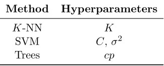
Table 3: Hyperparameters tuned via the model selection procedure outlined in Section 2.6.
σ2 is a parameter in the radial basis function kernel,K(xi,xj) = exp(
kxi−xjk
σ2 ). cp
is a complexity parameter related to the depth of the decision tree.
2.7 Extensions to Multiple Imputation
Thus far, we have described opt.impute methods for single imputation which output a single completed data set. On the other hand, multiple imputation methods output m≥2 different completed data sets for a single missing data problem. Afterwards, analysis is performed on each of the m data sets separately, and the results are pooled (Little and Rubin, 1987). For some applications, multiple imputation is preferred because it captures the variation in missing data imputation, which enables us to compute confidence intervals for downstream models trained on the imputed data sets. In addition, the pooled results from models fit on multiple imputed data sets may provide better point estimates than models fit on a single imputed data set in some cases.
To extend opt.impute to produce multiple imputations, we generate m warm starts using a probabilistic procedure, run opt.knn, opt.svm, or opt.tree from these starting points, and output the full set ofmcompleted data sets. These warm starts can be generated from sample draws under a previously estimated posterior distribution; an example would be using outputs from the mice procedure. This provides us with a representative set of imputations found by theopt.imputealgorithm, which converges to local optima. We refer to the multiple imputation method as opt.mi. In the computational experiments, we use the benchmark multiple imputation method miceto generate the warm starts.
Note that there are other possible ways of adapting opt.impute to the multiple im-putation schema. We may introducem instances of artificial noise in the observed values, and solve the resulting optimization problems. Alternatively, we may run opt.impute on
m bootstrapped samples of the original data set. Afterwards, we can analyze each of the
m imputed data sets separately and pool the results as before.
3. Real-World Data Experiments
3.1 Experimental Setup
To test the accuracy of the proposed missing data imputation method, we run a series of computational experiments on data sets taken from the UCI Machine Learning Repository for both regression and classification tasks. The data sets cover a range of number of obser-vationsnand number of featuresp, potentially mixed with both continuous and categorical variables. The numbers of continuous (p0) and categorical (p1) variables in each of these data sets are given in Table 10.
In these experiments, we use full data sets in which all entries are known, and we generate patterns of missing data for various percentages ranging from 10% to 50%. We take the full data setsXthat have no missing entries to be the ground truth. We run some of the most commonly-used and state-of-the-art methods for data imputation on these data sets to predict the missing values and compare against our optimization based imputation methods. The individual methods in this comparison are:
1. Mean Impute(mean): The simplest imputation method. For each missing valuexid,
imputes the mean of all known values in dimensiond.
2. Predictive-Mean Matching(pmm): An iterative method which imputes missing val-ues from known valval-ues in a given dimension using linear regressions. It is commonly used for multiple imputation and can be generalized to multiple missing dimensions using the chained equations process (Buuren and Groothuis-Oudshoorn, 2011). Im-plemented using the MICEpackage inR.
3. Bayesian PCA(bpca): A missing data estimation method based on Bayesian prin-cipal component analysis (Oba et al., 2003). Implemented using the pcaMethods package inR.
4. K-Nearest Neighbors (knn): A single-step, greedy method which imputes missing values using the K-nearest neighbors of an observation based upon Euclidean dis-tance. The candidate neighbors must have non-missing values in the imputed feature. Averaged distance is used if some other coordinates are missing. Implemented using theimputepackage inR.
5. IterativeK-Nearest Neighbors(iknn): Implemented inRand Julia, based on the description in the original papers (Br´as and Menezes, 2007; Caruana, 2001) .
6. Optimal Impute(opt.impute): All sub-methods below use warm starts including: mean, knn, bpca and five random starts where the values are imputed by a random sampling of the non-missing observations of that feature. The imputation which results in the lowest objective value is selected for each method.
(b) SVM Regression and Classification based (opt.svm): This method solves the maximum margin support vector machine problem (11) using a radial basis function kernel. For continuous variables, we use -support vector regression; for categorical variables, we use classical support vector machines. These prob-lems were solved using coordinate descent methods. The implementation was in
Juliausing thescikit-learn package inPython.
(c) Decision Tree based (opt.tree): This method solves the optimal decision-tree problem (15). For continuous variables, a single-leaf regularized regression tree is used; for categorical variables, a fast coordinate descent-based algorithm for solving Optimal Classification Trees is used (Bertsimas and Dunn, 2017). We run coordinate descent for the imputation problems. The implementation was
inJuliausing the packages glmnetandOptimalTrees.
In addition, we consider two composite methods: opt.cv, which selects the best method from opt.knn,opt.svm, andopt.tree; andbenchmark.cv, which selects the best method from mean, pmm, bpca, knn, and iknn. These composite methods use the cross-validation procedure described in Section 2.6. To generate the validation set for each missing data problem, we randomly sample an additional 10% of the entries to be hidden under the MCAR assumption. After running each individual method, we select the one that gives the lowest MAE on the validation set. We re-run this method on the original missing data set to obtain the final imputation.
Each imputation method was run for a maximum time limit of 12 hours on each data set. The quality of the imputations is evaluated using the same MAE and RMSE metrics defined in Section 2.6. For each of the opt.impute methods, we also record and present the convergence in objective value and MAE to show the progress over the iterations.
3.1.1 Missing Pattern
Because the mechanism which generates the pattern of missing data can affect imputa-tion quality, we run experiments under two different missing data mechanisms: missing completely at random (MCAR) and not missing at random (NMAR). These statistical as-sumptions are summarized in Table 4. The MCAR assumption implies that the missing pattern is completely independent from both the missing and observed values. The NMAR assumption implies that the missing pattern depends upon the missing values. There is an intermediate type of assumption, missing at random (MAR), which implies that the missing pattern depends only upon the observed values, but not upon the missing values. Because this assumption is less general than NMAR, we do not consider this mechanism for our experiments.
To generate MCAR patterns of missing data, we randomly sample a subset of the entries in X to be missing, assuming that each entry is equally likely to be chosen. The NMAR patterns are generated by sampling missingness indicators as independent Bernoulli random variables where each probability pid equals the probability that a normal random variable N(xid, ) is greater than a particular threshold for dimension d. The threshold for each
Mechanism of Missing Data Assumption
Missing Completely at Random (MCAR) f(M|Xobs,Xmiss) =f(M) Missing at Random (MAR) f(M|Xobs,Xmiss) =f(M|Xobs)
Not Missing at Random (NMAR) f(M|Xobs,Xmiss) is a function ofXmiss
Table 4: Statistical assumptions of mechanisms used to generate patterns of missing data Mfor data setX. Here, we suppose thatf is the underlying density of the missing pattern, andXobs,Xmissare the observed and missing components of the data set, respectively.
Note that regardless of the missing data scenarios generated for the experiments, in order to make fair comparisons, we always use MCAR as the generating mechanism for cross-validation.
3.1.2 Downstream Tasks
For 10 data sets from the UCI Machine Learning Repository, we run further experiments to evaluate the impact of these imputations on the intended downstream machine learning tasks. This selection includes a representative sample of 5 data sets for regression and 5 data sets for classification, with dependent variable observations Y ∈Rn and Y ∈ {0,1}n
respectively. We evaluate both single and multiple imputation methods in these experi-ments.
For single imputation, we consider opt.cv and benchmark.cv. First, we divide each downstream data set using a 50% training/testing split. Next, we randomly sample a fixed percentage of the entries in X to be missing completely at random, ranging from 10% to 50%. For each missing percentage, we impute the missing values in the training set and then fit standard machine learning algorithms to obtain a classification or regression model. We impute the missing values in the testing set by running the imputation methods on the full data set. For the regression tasks, we fit cross-validated LASSO and SVR models and compute the out-of-sample accuracy on the imputed testing set. For the classification tasks, we fit cross-validated SVM and Optimal Trees models and compute the out-of-sample R2
on the imputed testing set.
We also evaluate the performance of multiple imputation methods on the downstream tasks. In these experiments, we consider the following methods:
1. Multivariate Imputation by Chained Equations (mice): An iterative method which imputes each dimension with missing values one at a time drawing from distri-butions fully conditional on the other variables. We use predictive mean matching for continuous variables and logistic regression for categorical variables. This process is repeated to generate m fully imputed data sets. Implemented via the MICE package inR.
imputed data sets. We use warm starts produced bymice, and the best model among
K-NN, SVM, and trees is selected initially via cross-validation.
For bothmiceandopt.mi, we generatem= 5 multiple imputations for the training set and fit an ensemble of predictive models on these completed training sets. We make predictions on the test set by averaging the predictions from the model ensemble. For the classification tasks, we use a threshold value of 0.5. We run this experiment 100 times with different training/testing splits and distributions of missing values for each data set and report the averaged out-of-sample of the predictive models.
3.2 Results
We run the methods on 84 data sets from the UCI Machine Learning Repository. These data sets range in size from n = 23 to 5,875 observations and dimensionp = 2 to 124. In the following sections, we first show the convergence for each of the opt.imputemethods is fast and generally leads to a decrease in MAE. Next, we demonstrate that the quality of the imputations is significantly higher foropt.imputecompared to the reference methods, and that this leads to improved performance on downstream classification and regression tasks. We further discuss the sensitivity of imputation quality to the model parameters (K,
cp, C), warm starts, descent method (BCD or CD), and data characteristics including the missing pattern. Finally, we compare the computational burden of each method.
3.2.1 Convergence
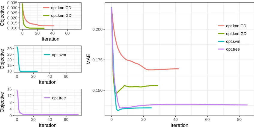
Figure 1 represents the change in objective value and MAE over the iterations for each of the opt.impute methods based on mean warm start, using iris data set as an example. We present results for opt.knn (CD and BCD), opt.svm (CD), and opt.tree(CD). The convergence is relatively fast for all methods; in particular, the BCD algorithm for K -NN converges significantly faster than the CD algorithm. When comparing the change in MAE, the value generally monotonically decreases with each iteration in concordance with the change in objective, especially during the first few iterations. In some paths, MAE increases slightly after a certain point. RMSE exhibits the same behavior and is therefore not plotted. This suggests a potential issue of overfitting to the known observations, which may be remedied by regularization or early stopping. In summary, the solution paths illustrate: 1) convergence is often fast, and 2) the objective functions are decent proxies for out-of-sample MAEs, and 3) imputation quality for each first-order method generally improves until convergence.
In general, we found that the BCD algorithm for opt.knndid not significantly improve upon imputation accuracy compared to the CD algorithm, but only improved upon speed. Because the BCD algorithms do not scale as well, we restricted our analysis to the CD algorithms foropt.svm andopt.tree.
3.2.2 Imputation Accuracy
0.010 0.015 0.020 0.025 0.030 0.035
0 20 40 60
Iteration
Objectiv
e opt.knn.CD
opt.knn.GD
10 15 20 25 30
0 20 40 60
Iteration
Objectiv
e
opt.svm
0 4 8 12 16
0 20 40 60
Iteration
Objectiv
e
opt.tree
0.150 0.175 0.200
0 20 40 60 80
Iteration
MAE
opt.knn.CD
opt.knn.GD
opt.svm
opt.tree
MAE (i.e., best imputation accuracy) is bolded. Among all data sets, at least one of the opt.impute methods obtains the lowest MAE in 76.2% of the data sets, followed by iknn and bpcaimputation methods with 9 and 4 wins each. Comparatively, mean,knn, andpmm impute have the weakest performances. Among the opt.impute methods, the tree based model achieves the lowest MAE in most data sets.
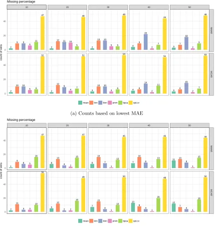
We repeat this experiment for other percentages of missing data with the winning counts summarized in Figure 2, using opt.cv as our proposed method. We show the number of times that each method achieves the best overall imputation with lowest MAE and RMSE under five different missing data percentages, as well MCAR and NMAR scenarios. In all missing data scenarios, our proposed method produces the best imputations in more than half of the data sets according to both performance metrics. Among the comparator methods,meanandpmmare generally among the weaker ones. When MAE is the metric, the heuristic method iknn performs the best among the benchmark methods, suggesting that the idea of iteratively updating the imputed values have merits. At higher percentages of missing values (the right-most subfigures), bpca improves in its performance when RMSE is the metric of evaluation, but still not as strong as opt.cv.
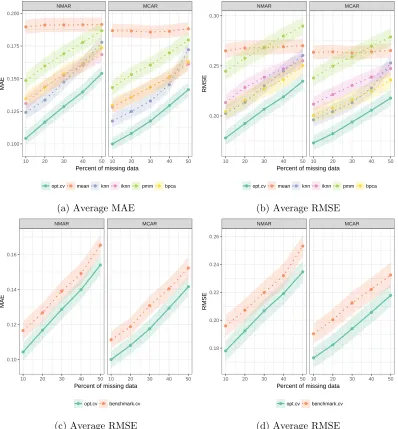
In Figure 3, we present summary results of the MAE and RMSE values as geometric means across all data sets for each missing percentage and missing data mechanism, with the confidence bands representing one geometric standard deviation multiplied above and divided below by the mean. Comparatively,opt.cvachieves the lowest average MAE and RMSE values for all missing percentages. At the 10% missing data percentage, the average MAE of the opt.cv imputations is 0.100, a reduction of 14.9% from the average MAE of 0.118 obtained by the best benchmark method knn. As missing percentages increase, opt.cvremains the most accurate imputation method, with the average MAE of 0.142 at 50% missing, a reduction of 12.1% from the average MAE of 0.172 obtained by the next best methodknn. The performance of opt.cvrelative to benchmark ones does not appear to differ drastically between the MCAR and NMAR scenarios, with overall higher MAE for NMAR across most methods, as expected.
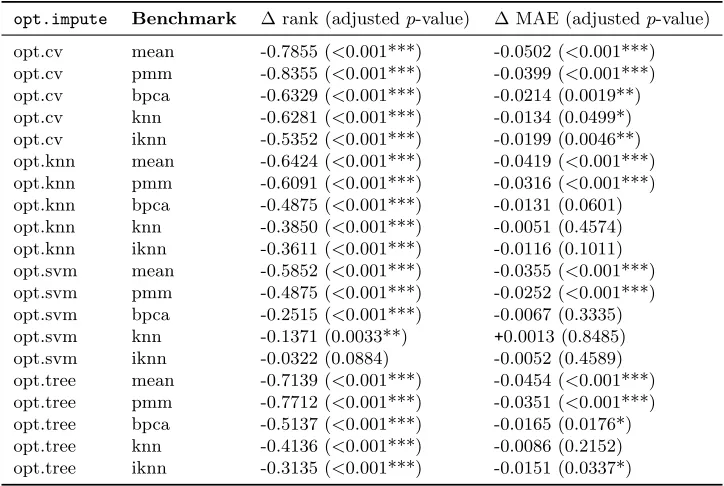
To isolate the effect of each individual method from the cross-validation procedure, we further summarize the results by comparing one method at a time against the benchmark ones. Table 5 presents the statistical comparisons between each opt.impute method and each benchmark method. We conduct pairwise Wilcoxon signed rank tests and paired t-tests between each pair of methods. When comparing opt.cv against the benchmark methods, our proposed cross-validated method achieves statistically significant lower rank and lower MAE compared to each benchmark. For each individual opt.impute method, with the exception of opt.svmagainst heuristiciknn, theopt.imputeone has statistically significant lower rank than every benchmark. The decrease in MAE is still statistically significant whenmean,bpca, andpmmare comparators, but no longer statistically significant when compared to knn or iknn. This suggests that each of the proposed methods holds its own against most benchmark ones, especially under rank comparisons, but the cross-validation procedure adds another layer of improvement in imputation quality.
47 2 9 9 6 11 52 2 10 10 5 6 46 2
12 11 10
5 52 2 12 9 4 7 48 2 13 13 5 5 54 3 10 10 3 6 44 4 9 22 2 7 51 4 6 14 2 11 48 3 7 18 2 9 53 3 6 15 2 7
10 20 30 40 50
NMAR MCAR 0 20 40 0 20 40
count of wins
mean knn iknn pmm bpca opt.cv
Missing percentage
(a) Counts based on lowest MAE
47 1 9 6 5 16 56 2 11 3 3 10 47 6 13 4 2 15 49 5 12 2 2 16 45 6 16 7 1 12 50 7 15 4 1 10 45 7 16 8 1 13 48 13 8 4 1 20 44 11 13 8 1 15 50 12 7 4 1 18
10 20 30 40 50
NMAR MCAR 0 20 40 0 20 40
count of wins
mean knn iknn pmm bpca opt.cv
Missing percentage
(b) Counts based on lowest RMSE
Table 5: Pairwise Wilcoxon signed-rank tests and t-tests between opt.impute and bench-mark methods, with thep-values adjusted for multiple comparisons.
opt.impute Benchmark ∆ rank (adjustedp-value) ∆ MAE (adjustedp-value)
opt.cv mean -0.7855 (<0.001***) -0.0502 (<0.001***) opt.cv pmm -0.8355 (<0.001***) -0.0399 (<0.001***) opt.cv bpca -0.6329 (<0.001***) -0.0214 (0.0019**) opt.cv knn -0.6281 (<0.001***) -0.0134 (0.0499*) opt.cv iknn -0.5352 (<0.001***) -0.0199 (0.0046**) opt.knn mean -0.6424 (<0.001***) -0.0419 (<0.001***) opt.knn pmm -0.6091 (<0.001***) -0.0316 (<0.001***) opt.knn bpca -0.4875 (<0.001***) -0.0131 (0.0601) opt.knn knn -0.3850 (<0.001***) -0.0051 (0.4574) opt.knn iknn -0.3611 (<0.001***) -0.0116 (0.1011) opt.svm mean -0.5852 (<0.001***) -0.0355 (<0.001***) opt.svm pmm -0.4875 (<0.001***) -0.0252 (<0.001***) opt.svm bpca -0.2515 (<0.001***) -0.0067 (0.3335) opt.svm knn -0.1371 (0.0033**) +0.0013 (0.8485) opt.svm iknn -0.0322 (0.0884) -0.0052 (0.4589) opt.tree mean -0.7139 (<0.001***) -0.0454 (<0.001***) opt.tree pmm -0.7712 (<0.001***) -0.0351 (<0.001***) opt.tree bpca -0.5137 (<0.001***) -0.0165 (0.0176*) opt.tree knn -0.4136 (<0.001***) -0.0086 (0.2152) opt.tree iknn -0.3135 (<0.001***) -0.0151 (0.0337*)
Further,opt.cvachieves highest imputation accuracy in more than 78.6% of the data sets compared to benchmark.cv.
3.2.3 Performance on Downstream Tasks
Next, we evaluate the performance of standard machine learning algorithms for classification and regression trained on the imputed data. We consider the data sets in Table 6, which were selected as a representative subsample from the UCI Machine Learning Repository data sets. These data sets range in size, havingn= 150 to 5,875 observations andp= 4 to 16 features. The difficulty of the regression or classification task on the completely known data set also varies widely. The baseline out-of-sample accuracy of an SVM model for the binary classification problems ranges from 77% to 100%, and the baseline out-of-sample
R2 of a LASSO model for the regression problems ranges from 0.09 to 0.82. For each of these data sets, the downstream tasks become more difficult as the missing data percentage increases.
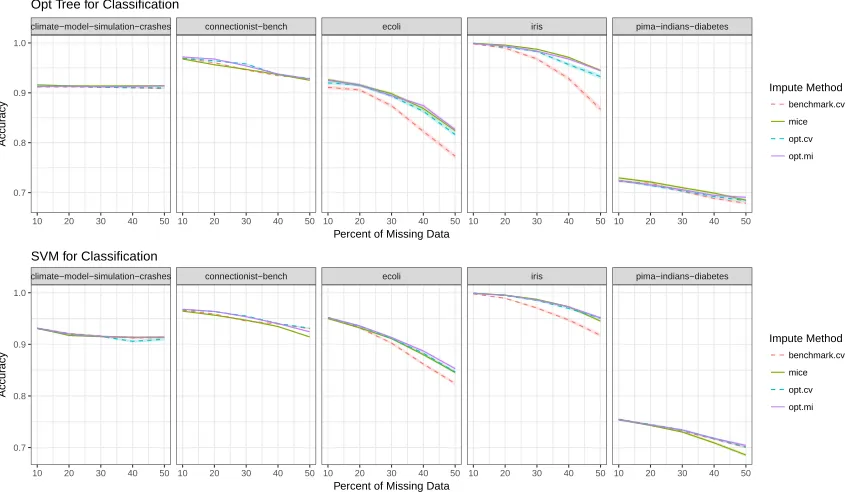
In Figure 4, we show how the imputation method chosen impacts the performance for downstream tasks, across different data sets and different missing data percentages. In Tables 7 and 8, we show pairwise t-test results, aggregating out-of-sample performance results by downstream task and missing percentage. These results include comparisons for both single and multiple imputation methods.
● ● ● ● ● ● ● ● ● ● ● ● ● ● ● ● ● ● ● ● ● ● ● ● ● ● ● ● ● ● ● ● ● ● ● ● ● ● ● ● ● ● ● ● ● ● ● ● ● ● ● ● ● ● ● ● ● ● ● ● NMAR MCAR
10 20 30 40 50 10 20 30 40 50 0.100
0.125 0.150 0.175 0.200
Percent of missing data
MAE
● opt.cv ● mean ● knn ● iknn ● pmm ● bpca
(a) Average MAE
● ● ● ● ● ● ● ● ● ● ● ● ● ● ● ● ● ● ● ● ● ● ● ● ● ● ● ● ● ● ● ● ● ● ● ● ● ● ● ● ● ● ● ● ● ● ● ● ● ● ● ● ● ● ● ● ● ● ● ● NMAR MCAR
10 20 30 40 50 10 20 30 40 50 0.20
0.25 0.30
Percent of missing data
RMSE
● opt.cv ● mean ● knn ● iknn ● pmm ● bpca
(b) Average RMSE
● ● ● ● ● ● ● ● ● ● ● ● ● ● ● ● ● ● ● ● NMAR MCAR
10 20 30 40 50 10 20 30 40 50 0.10
0.12 0.14 0.16
Percent of missing data
MAE
● opt.cv ● benchmark.cv
(c) Average RMSE
● ● ● ● ● ● ● ● ● ● ● ● ● ● ● ● ● ● ● ● NMAR MCAR
10 20 30 40 50 10 20 30 40 50 0.18
0.20 0.22 0.24 0.26
Percent of missing data
RMSE
● opt.cv ● benchmark.cv
(d) Average RMSE
Downstream Task Name (n, p) Baseline Accuracy orR2
Classification
climate-model-crashes (540, 18) 0.95 connectionist-bench (990, 10) 0.93
ecoli (336, 8) 0.96
iris (150, 4) 1.00
pima-indians-diabetes (768, 8) 0.77
Regression
abalone (4177, 7) 0.51
auto-mpg (392, 8) 0.82
housing (506, 13) 0.71
parkinsons-telemonitoring-total (5875, 16) 0.09 wine-quality-white (4898, 11) 0.27
Table 6: Data sets considered for downstream regression and classification tasks. For clas-sification tasks, we list the average baseline out-of-sample accuracy of an SVM model fit on the full data set, and for regression tasks, we list the average baseline out-of-sampleR2 of a LASSO model fit on the full data set.
accuracy and R2 is monotonically increasing with the missing percentage. At 50% missing data, the average improvement in out-of-sample accuracy is 1.7% for classification tasks, and the average improvement in out-of-sampleR2 is 0.024 for regression tasks.
For the multiple imputation methods, we observe that the improvement of opt.miover mice is statistically significant for all missing percentages in the regression tasks, and 3/5 missing percentages in the classification tasks. At the 50% missing percentage, the average improvement is 0.5% in sample accuracy for classification tasks and 0.010 in out-of-sampleR2 for regression tasks. While these improvements are smaller than those for single imputation, they are significant at thep= 0.001 level.
Overall, these results suggest that opt.impute leads to gains in out-of-sample perfor-mance in both single and multiple imputation settings. The relative improvements are consistently greatest at the highest missing percentages, where the imputation method se-lected has the largest impact on the downstream performance.
Finally, we compare the performance of single vs multiple imputation for opt.impute. We observe that the improvement of opt.mioveropt.cvis statistically significant in 8/10 scenarios, with the largest improvements occurring at the highest missing percentages. At the 50% missing percentage, the average improvement is 0.4% in out-of-sample accuracy for classification tasks and 0.017 in out-of-sampleR2 for regression tasks. These improvements are similar to the gains in performance overmice.
3.2.4 Sensitivity to Parameters
Model performance can be impacted by various parameters. For a specific data set and model, the performance can be sensitive to hyperparameters such as the number of neighbors
climate−model−simulation−crashes connectionist−bench ecoli iris pima−indians−diabetes
10 20 30 40 50 10 20 30 40 50 10 20 30 40 50 10 20 30 40 50 10 20 30 40 50 0.7
0.8 0.9 1.0
Percent of Missing Data
Accur
acy
Impute Method
benchmark.cv
mice
opt.cv
opt.mi Opt Tree for Classification
climate−model−simulation−crashes connectionist−bench ecoli iris pima−indians−diabetes
10 20 30 40 50 10 20 30 40 50 10 20 30 40 50 10 20 30 40 50 10 20 30 40 50 0.7
0.8 0.9 1.0
Percent of Missing Data
Accur
acy
Impute Method
benchmark.cv
mice
opt.cv
opt.mi SVM for Classification
(a) Average out-of-sample accuracy values with standard errors of Optimal Trees and SVM models
abalone auto−mpg housing parkinsons−telemonitoring−total wine−quality−white
10 20 30 40 50 10 20 30 40 50 10 20 30 40 50 10 20 30 40 50 10 20 30 40 50 0.0
0.2 0.4 0.6 0.8
Percent of Missing Data
OSR2
Impute Method
benchmark.cv
mice
opt.cv
opt.mi SVR for Regression
abalone auto−mpg housing parkinsons−telemonitoring−total wine−quality−white
10 20 30 40 50 10 20 30 40 50 10 20 30 40 50 10 20 30 40 50 10 20 30 40 50 0.0
0.2 0.4 0.6 0.8
Percent of Missing Data
OSR2
Impute Method
benchmark.cv
mice
opt.cv
opt.mi LASSO for Regression
(b) Average out-of-sampleR2 values with standard errors of SVR and LASSO models
∆ Out-of-Sample Accuracy (adjustedp-value)
Missing % opt.mi-mice opt.cv-benchmark.cv opt.mi-opt.cv
10 -0.0001 (1.0000) 0.0016 (0.0059**) 0.0006 (0.2076) 20 0.0018 (0.0059**) 0.0026 (<0.001***) 0.0008 (0.2076) 30 0.0005 (0.9858) 0.0082 (<0.001***) 0.0002 (1.0000) 40 0.0018 (0.0491*) 0.0113 (<0.001***) 0.0043 (<0.001***) 50 0.0052 (<0.001***) 0.0171 (<0.001***) 0.0038 (<0.001***)
Table 7: Pairwise t-tests between opt.impute and benchmark methods for downstream classification tasks, with thep-values adjusted for multiple comparisons.
∆ Out-of-SampleR2 (adjustedp-value)
Missing % opt.mi-mice opt.cv-benchmark.cv opt.mi-opt.cv
10 0.0014 (<0.001***) 0.0034 (<0.001***) 0.0013 (<0.001***) 20 0.0029 (<0.001***) 0.0113 (<0.001***) 0.0027 (<0.001***) 30 0.0071 (<0.001***) 0.0161 (<0.001***) 0.0077 (<0.001***) 40 0.0085 (<0.001***) 0.0195 (<0.001***) 0.0108 (<0.001***) 50 0.0097 (<0.001***) 0.0237 (<0.001***) 0.0174 (<0.001***)
Table 8: Pairwise t-tests between opt.impute and benchmark methods for downstream regression tasks, with thep-values adjusted for multiple comparisons.
percentage may affect the imputation quality as well. This section explores how these parameters impact the imputation quality.
We found that all of the imputation model hyperparameters that we investigated affect imputation accuracy. Figure 5 shows the relationship between the hyperparameters and MAE for various data sets and missing patterns. For opt.knn (CD and BCD), the out-of-sample MAE first decreases and then increases as the hyperparameter increases. When K
reaches the sample size, the imputation is equivalent to mean imputation. For opt.svm, the imputation accuracy remains relatively constant with respect to changes in parameter
C after a certain threshold. There were no external parameters for trees, as the trees in each step were pruned during the training process. Overall, these plots suggest that the opt.impute methods are relatively robust even if their hyperparameters are not known exactly.
k=22 k=10
k=40
0.075 0.100 0.125 0.150 0.175 0.200
0 25 50 75 100
k
MAE
(a)K inopt.knn.CD
k=19 k=46 k=13
0.075 0.100 0.125 0.150 0.175 0.200
0 25 50 75 100
k
MAE
(b)K inopt.knn.BCD
C=0.95 C=0.99 C=0.65
0.075 0.100 0.125 0.150 0.175 0.200
0.00 0.25 0.50 0.75 1.00
C
MAE
(c)C foropt.svm
Figure 5: Sensitivity of MAE to the choice of K for the number of neighbors for K-NN coordinate descent,K-NN block coordinate descent, and the trade-off parameter
Cfor SVM in data setiris. The colors represent different missing data percent-ages. The parameter value that achieves lowest MAE is labeled for each missing data percentage.
3.2.5 Computational Speed
Next, we compare the computational time required for all imputation methods across a selection of six UCI data sets and missing data patterns. Each method was run on a single thread of a machine with an Intel Xeon CPU E5-2650 (2.00 GHz) Processor and limited to 8 GB RAM with a time limit of 4 hours. For variousopt.impute methods, we report the running times for mean warm starts, as multiple warm starts can be trivially parallelized. The results are shown below in Table 9.
Mean imputation is almost instantaneous and is therefore not presented in the table. For small-scale problems on the iris data set, all imputation methods finish quickly. As the data dimension p increases (for example, in the libras-movement data set), most opt.impute methods scale better than the pmm method. As the sample size n increases,
opt.knn.CDalso scales better thanpmm, as seen inbanknote-authenticationandskin-segmentation. Among the opt.impute methods, tree based imputation scales very well with respect to
sample size nbut not dimension p. Despite its high imputation quality, SVM based impu-tation scales relatively poorly with respect to bothnandp. Among the proposed methods, opt.knn.CDhas the best scalability in both nand p.
In particular, when comparing coordinate descent and block coordinate descent methods, the former performs best when the data size is large. When n is in the 100,000s, the coordinate descent method still converges within one hour (see skin-segmentation). For the block coordinate descent method, each iteration requires solving a separate system of linear equations for each continuous dimension, or an integer optimization problem for each of the categorical dimensions. On the other hand, the main bottleneck of opt.knn.CD is computing the K-NN assignment on X to update Z each iteration, which requires only
Time (in seconds)
Benchmark opt.impute
Name (n, p) Missing % bpca knn pmm knn.CD knn.BCD svm.CD tree.CD
iris (150, 4)
10 0.802 0.088 0.353 0.006 0.023 0.131 0.049 30 1.717 0.446 0.474 0.036 0.041 0.498 0.091 50 1.875 0.736 0.334 0.085 0.097 0.762 0.062 banknote-authen. (1372, 4)
10 2.262 2.552 1.717 0.261 1.285 3.269 0.046 30 14.058 14.914 1.911 0.772 4.981 15.625 0.116 50 17.820 16.889 2.141 1.578 17.573 15.280 0.159 libras-movement (360, 90)
10 2.624 0.088 0.353 0.006 0.023 0.131 0.049 30 3.423 0.446 0.474 0.036 0.041 0.498 0.091 50 1.892 0.736 0.334 0.085 0.097 0.762 0.062 mushroom (5644, 76)
10 26.432 387.386 4782.855 8.037 72.169 1442.942 -30 46.726 8.134 1068.476 12.818 17.572 - -50 63.556 10.155 893.243 10.511 12.948 - -skin-segmentation (245057, 3)
10 392.310 1144.120 12193.105 1144.144 144.679 - 9.574
30 450.584 1380.138 - 1420.641 - - 15.616
50 615.037 2503.464 - 2582.102 - - 17.818
cnae-9 (1080, 856)
10 30.310 13.038 - 12.701 12.727 -
-30 58.205 13.970 - 13.931 13.972 -
-50 126.059 14.361 - 14.284 14.343 -