Noisy Sparse Subspace Clustering
Yu-Xiang Wang [email protected]
Machine Learning Department Carnegie Mellon University Pittsburgh, PA 15213
Huan Xu [email protected]
Department of Mechanical Engineering National University of Singapore Singapore 117576
Editor:Matthias Hein
Abstract
This paper considers the problem of subspace clustering under noise. Specifically, we study the behavior of Sparse Subspace Clustering (SSC) when either adversarial or random noise is added to the unlabeled input data points, which are assumed to be in a union of low-dimensional subspaces. We show that a modified version of SSC is provably effective
in correctly identifying the underlying subspaces, even with noisy data. This extends theoretical guarantee of this algorithm to more practical settings and provides justification to the success of SSC in a class of real applications.
Keywords: Subspace clustering, robustness, stability, compressive sensing, sparse
1. Introduction
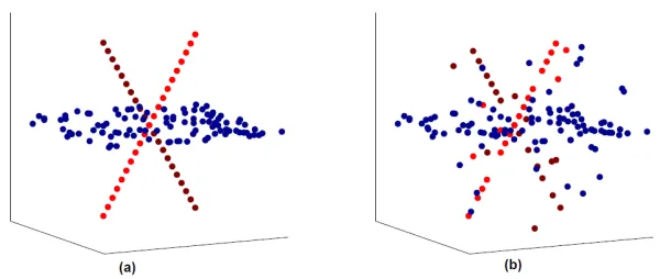
Subspace clustering is a problem motivated by many real applications. It is now widely known that many high dimensional data including motion trajectories (Costeira and Kanade, 1998), face images (Basri and Jacobs, 2003), network hop counts (Eriksson et al., 2012), movie ratings (Zhang et al., 2012) and social graphs (Chen et al., 2014) can be modeled as samples drawn from the unionof multiple low-dimensional linear subspaces (illustrated in Figure 1). Subspace clustering, arguably the most crucial step to understand such data, refers to the task of clustering the data into their original subspaces and uncovering the underlying structure of the data. The partitions correspond to different rigid objects for motion trajectories, different people for face data, subnets for network data, like-minded users in movie database and latent communities for social graph.
Figure 1: Exact (a) and noisy (b) data in union-of-subspace
et al., 2010, 2013) and Sparse Subspace Clustering (SSC) (Elhamifar and Vidal, 2009, 2013). For a comprehensive survey and comparisons, we refer the readers to the tutorial (Vidal, 2010). Among these algorithms, SSC is known to enjoy superb empirical performance,even for noisy data. For example, it is the state-of-the-art algorithm for motion segmentation on Hopkins155 benchmark (Tron and Vidal, 2007; Elhamifar and Vidal, 2009), and has been shown to be more robust than LRR as the number of clusters increase (Elhamifar and Vidal, 2013).
The key idea of SSC is to represent each data point by a sparse linear combination of the remaining data points using `1 minimization. Without introducing the notations (which is deferred in Section 3), the noiseless and noisy versions of SSC solve respectively
min ci
kcik1 s.t. xi=X−ici, and min ci
kcik1+λ
2kxi−X−icik
2,
for each data column xi, and the hope is that ci will be supported only on indices of the data points from the same subspace as xi. While this formulation is for linear subspaces, affine subspaces can also be dealt with by augmenting data points with an offset variable 1. Effort has been made to explain the practical success of SSC by analyzing the noiseless version. Elhamifar and Vidal (2010) show that under certain conditions,disjoint subspaces (i.e., they are not overlapping) can be exactly recovered. A recent geometric analysis of SSC (Soltanolkotabi et al., 2012) broadens the scope of the results significantly to the case when subspaces can be overlapping. However, while these analyses advanced our understanding of SSC, one common drawback is that data points are assumed to be lying
exactlyon the subspaces. This assumption can hardly be satisfied in practice. For example, motion trajectories data are only approximately of rank-4 due to perspective distortion of camera, tracking errors and pixel quantization (Costeira and Kanade, 1998); similarly, face images are not precisely of rank-9 since human faces are at best approximatedby a convex body (Basri and Jacobs, 2003).
same geometric gap determines whether SSC succeeds for the noiseless case. Indeed, when the noise vanishes, our results reduce to the noiseless case results of Soltanolkotabi et al..
While our analysis is based upon the geometric analysis of Soltanolkotabi et al. (2012), the analysis is more involved: In SSC, sample points are used as the dictionary for sparse recovery, and therefore noisy SSC requires analyzing a noisy dictionary. We also remark that our results on noisy SSC areexact, i.e., as long as the noise magnitude is smaller than a threshold, the recovered subspace clusters are correct. This is in sharp contrast to the majority of previous work on structure recovery for noisy data where stability/perturbation bounds are given—i.e., the obtained solution isapproximately correct, and the approxima-tion gap goes to zero only when the noise diminishes.
Lastly, we remark that an independently developed work (Soltanolkotabi et al., 2014) analyzed the same algorithmunder a statistical modelthat generates the data. In contrast, our main results focus on the cases when the data are deterministic. Moreover, when we specialize our general result to the same statistical model, we show that we can handle a significantly larger amount of noise under certain regimes.
The paper is organized as follows. In Section 2, we review previous and ongoing works related to this paper. In Section 3, we formally define the notations, explain our method and the models of our analysis. Then we present our main theoretical results in Section 4 with examples and remarks to explain the practical implications of each theorem. In Sec-tion 5 and 6, proofs of the deterministic and randomized results are provided. We then evaluate our method experimentally in Section 7 with both synthetic data and real-life data, which confirms the prediction of the theoretical results. Lastly, Section 8 summa-rizes the paper and discuss some open problems for future research in the task of subspace clustering.
2. Related works
In this section, we review previous and ongoing theoretical studies on the problem of sub-space clustering.
2.1 Nominal performance guarantee for noiseless data
Most previous analyses concern about the nominal performance of a particular subspace clustering algorithm with noiseless data. The focus is to relax the assumptions on the underlying subspaces and data generation.
A number of methods have been shown working under theindependent subspace assump-tion including the early factorizaassump-tion-based methods (Costeira and Kanade, 1998; Kanatani, 2001), LRR (Liu et al., 2010) and the initial guarantee of SSC (Elhamifar and Vidal, 2009). Recall that the data points are drawn from a union of subspaces, the independent subspace
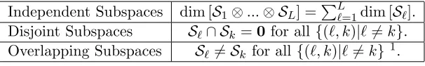
Independent Subspaces dim [S1⊗...⊗ SL] =PL
`=1dim [S`]. Disjoint Subspaces S`∩ Sk =0 for all {(`, k)|`6=k}. Overlapping Subspaces S`6=Sk for all{(`, k)|`6=k}1.
Table 1: Comparison of conditions on the underlying subspaces.
Disjoint subspace assumption only requires pairwise linear independence, and hence is more meaningful in practice. To the best of our knowledge, only GPCA (Vidal et al., 2005) and SSC (Elhamifar and Vidal, 2010, 2013) have been shown to provably handle the data underdisjoint subspaceassumption. GPCA however is not a polynomial time algorithm. Its computational complexity increases exponentially with respect to the number and dimension of the subspaces.
Soltanolkotabi et al. (2012) developed a geometric analysis that further extends the performance guarantee of SSC, and in particular it covers some cases when the underlying subspaces areoverlapping, meaning that two subspaces can even share a basis. The analysis reveals that the success of SSC relies on the difference of two geometric quantities (inradius
r and incoherence µ) to be greater than 0, which leads to by far the most general and strongest theoretical guarantee for noiseless SSC. A summary of these assumptions on the subspaces and their formal definition are given in Table 1.
We remark that our robust analysis extends from Soltanolkotabi et al. (2012) and there-fore is inherently capable of handling the same range of problems, namely disjoint and overlapping subspaces. This is formalized later in Section 4.
2.2 Robust performance guarantee
Previous studies of the subspace clustering under noise have been mostly empirical. For instance, factorization, spectral clustering and local affinity based approaches, which we mentioned above, are able to produce a (sometimes good) solution even for noisy real data. Convex optimization based approaches like LRR and SSC can be naturally reformulated as a robust method by relaxing the hard equality constraints to a penalty term in the objective function. In fact, the superior results of SSC and LRR on motion segmentation and face clustering data are produced using the robust extension in Elhamifar and Vidal (2009) and Liu et al. (2010) instead of the well-studied noiseless version.
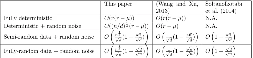
As of writing, there have been very few subspace clustering methods that is guaranteed to work when data are noisy. Besides the conference version of the current paper (Wang and Xu, 2013), an independent work (Soltanolkotabi et al., 2014) also analyzed SSC under noise. Subsequently, there has been noisy guarantees for other algorithms, e.g., thresholding based approach (Heckel and B¨olcskei, 2013) and orthogonal matching pursuit (Dyer et al., 2013). The main difference between our work and Soltanolkotabi et al. (2014) is that our guarantee works for a more general set of problems when the data and noise may not be
This paper (Wang and Xu, 2013)
Soltanolkotabi et al. (2014) Fully deterministic O(r(r−µ)) O(r(r−µ)) N.A. Deterministic + random noise O((n/d)14(r−µ)) O(r−µ) N.A.
Semi-random data + random noise O
n14
√ d(1−
aff
√ d)
O√1
d(1−
aff
√ d)
O1−√aff
d
Fully-random data + random noise O
n14
√ d(1−
√ d √
n)
O√1 d(1−
√ d √
n)
O1−
√ d √
n
Table 2: Comparison of the level of noise tolerable for noisy subspace clustering methods. Note that “aff” is theunnormalized affinity defined in Soltanolkotabi et al. (2012)
.
random, whereas the key arguments in the proof in Soltanolkotabi et al. (2014) rely on the assumption that data points are uniformly distributed on the unit sphere within each subspace, which corresponds to the “semi-random model” in our paper. As illustrated in Elhamifar and Vidal (2013, Figure 9 and 10), the semi-random model is not a good fit for either the motion segmentation and the face clustering data sets, as in these data sets there is a fast decay in the singular values of each subspace. The uniform distribution assumption becomes even harder to justify as the dimension dof each subspace gets larger—a regime where the analysis in Soltanolkotabi et al. (2014) focuses on.
Moreover, with a minor modification in our analysis that sharpens the bound of the tuning parameter that ensures the solution is non-trivial, we are able to get a result that is stronger than Soltanolkotabi et al. (2014) in cases when the dimension of each subspace
d ≤ O(√n) 2. This result extends the provably guarantee of SSC to a setting where the signal to noise ratio (SnR) is allowed to go to 0 as the ambient dimension gets large. In summary, we compare our results in terms of the level of noise that can be provably tolerated in Table 2. These comparisons are in the same setting modulo some slight differences in the noise model and successful criteria. It is worth noting that whend > O(√n), Soltanolkotabi et al. (2014)’s bound is sharper. We will provide more details in the Appendix.
Lastly, we note that the notion of robustness in this paper is confined to the noise/arbitrary corruptions added to the legitimate data. It is not the robustness against outliers in the data, unless otherwise specified. Handling outliers is a completely different problem. Solutions have been proposed for LRR in Liu et al. (2012) by decomposing a `2,1 norm column-wise
sparse components and for SSC in Soltanolkotabi et al. (2012) by objective value thresh-olding. However these results require non-outlier data points to be free of noise, therefore are not comparable to the study in this paper.
3. Problem setup
In this section, we specify the notations that will be use throughout the paper and explain the formal problem setup.
3.1 Notations
We denote the uncorrupted data matrix byY ∈Rn×N, where each column ofY (normalized to unit vector 3) belongs to a union ofL subspaces
S1∪ S2∪...∪ SL.
Each subspace S` is of dimensiond` and containsN` data samples withN1+N2+...+
NL =N. We observe the noisy data matrix X =Y +Z, where Z is some arbitrary noise matrix. Let Y(`) ∈ Rn×N` denote the selection of columns in Y that belongs to S
`, and denote the corresponding columns in X and Z by X(`) and Z(`) respectively. Without loss of generality, letX = [X(1), X(2), ..., X(L)] be ordered. In addition, we use subscript “−i” to represent a matrix that excludes column i, e.g.,X−(`i)= [x(1`), ..., xi(−`)1, x(i+1`) , ..., x(N`)
`].
Calli-graphic letters such as X,Y` represent the set containing all columns of the corresponding matrix (e.g.,X and Y(`)).
For any matrix X, P(X) represents the symmetrized convex hull of its columns, i.e.,
P(X) = conv(±X). Also let P−(`i) := P(X−(`i)) and Q(−`)i := P(Y−(`i)) for short. PS and
ProjS denote respectively the projection matrix and projection operator (acting on a set)
to subspaceS. Throughout the paper,k · krepresents 2-norm for vectors and operator norm for matrices; other norms will be explicitly specified (e.g.,k · k1,k · k∞).
3.2 Method and the criterion of success
Original SSC solves the linear program
min ci
kcik1 s.t. xi =X−ici, (3.1)
for each data point xi. Solutions are arranged into matrix C = [c1, ..., cN], then spectral clustering techniques such as Ng et al. (2002) are applied on the affinity matrix W =
|C|+|C|T (| · | represents entrywise absolute value). Note that when Z 6= 0, this method breaks down: indeed (3.1) may even be infeasible.
To handle noisy X, a natural extension is to relax the equality constraint in (3.1) and solve the following unconstrained minimization problem instead (Elhamifar and Vidal, 2013):
min ci
kcik1+λ
2kxi−X−icik
2. (3.2)
We will focus on Formulation (3.2) in this paper. Notice that (3.2) coincides with stan-dard LASSO. Yet, since our task is subspace clustering, the analysis of LASSO (mainly for the task of support recovery) does not extend to SSC. In particular, existing literature for LASSO to succeed requires the dictionaryX−i to satisfy the Restricted Isometry Prop-erty (RIP for short; Cand`es, 2008) or the Null-space property (Donoho et al., 2006), but neither of them is satisfied in the subspace clustering setup.4
3. We assume the normalization condition for ease of presentation. Our results can be extended to the case when each column of the noisy data pointsX=Y +Z is normalized, as well as the case where no normalizing is performed at all, under simple modifications to the conditions.
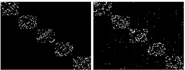
Figure 2: Illustration of LASSO-Subspace Detection Property/Self-Expressiveness Prop-erty. Left: SEP holds. Right: SEP is violated even though spectral clustering is likely to cluster this affinity graph perfectly into 5 blocks.
In the subspace clustering task, there is no single “ground-truth” C to compare the solution against. Instead, the algorithm succeeds if each sample is expressed as a linear combination of samples belonging to the same subspace, as the following definition states.
Definition 1 (LASSO Subspace Detection Property) We say the subspaces {S`}k `=1 and noisy sample points X from these subspaces obey LASSO subspace detection property with parameter λ, if and only if it holds that for all i, the optimal solution ci to (3.2)with
parameter λsatisfies:
(1) ci is not a zero vector, i.e., the solution is non-trivial, (2) Nonzero entries of ci
correspond to only columns of X sampled from the same subspace as xi.
This property ensures that the output matrixC and (naturally) the affinity matrixW are exactly block diagonal with each subspace cluster represented by a disjoint block. The property is illustrated in Figure 2. For convenience, we will refer to the second requirement alone as “Self-Expressiveness Property” (SEP), as defined in Elhamifar and Vidal (2013).
Note that the LASSO Subspace Detection Property is a strong condition. In practice, spectral clustering does not require the exact block diagonal structure for perfect segmen-tation (check Figure 8b in our simulation section for details). A caveat is that it is also not sufficient for perfect segmentation, since it does not guarantee each diagonal block forms a connected component. This is a known problem for SSC (Nasihatkon and Hartley, 2011), although we observe that in practice graph connectivity is usually not a big issue. Proving the high-confidence connectivity (even under probabilistic models) remains an open prob-lem, except for the almost trivial cases when the subspaces are independent (Liu et al., 2013; Wang et al., 2013).
3.3 Models of analysis:
4. Main results
In this section, we present our theoretical guarantee for LASSO-SSC under the four afore-mentioned models. We will start by describing subspace clustering for a fixed dataset where each data point can be perturbed by an arbitrary noise of bounded size. Then we will in-crementally add stochastic assumptions and state the corresponding results with conditions that reveal explicit dependence on parameters of the model.
4.1 Deterministic model
We start by defining two concepts adapted from the original proposal of Soltanolkotabi et al. (2012).
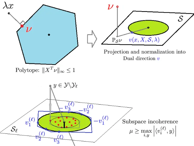
Definition 2 (Projected Dual Direction) Let ν be the optimal solution to the dual op-timization program5
max
ν hx, νi − 1 2λν
Tν, subject to: kXTνk
∞≤1;
and S is a low-dimensional subspace. The projected dual direction v is defined as
v(x, X,S, λ), kPSν
PSνk .
Definition 3 (Projected Subspace Incoherence Property) Compactly denote projected dual direction vi(`) =v(x(i`), X−(`i),S`, λ) and V(`) = [v(1`), ..., v
(`)
N`]. We say that vector set X` is µ-incoherent to other points if
µ≥µ(X`) := max y∈Y\Y`
kV(`)Tyk∞.
Here, µ measures the incoherence between corrupted subspace samples X` and clean data points in other subspaces (illustrated in Figure 4). As kyk = 1 by the normalization assumption, the range of µ is [0,1]. In case of random subspaces in high dimension, µ is close to zero. Moreover, as we will see later, for deterministic subspaces and random data points,µis proportional to their expected angular distance (measured by cosine of canonical angles).
Definition 2 and 3 differ from the dual direction and subspace incoherence property of Soltanolkotabi et al. (2012) in that we require a projection to a particular subspace to cater to the analysis of the noise case. Also, since they reduce to the original definitions when data are noiseless and λ → ∞, these definitions can be considered as a generalization of their original version.
Definition 4 (inradius) The inradius of a convex body P, denoted by r(P), is defined as the radius of the largest Euclidean ball inscribed in P.
The inradius of aQ(−`i)describes the dispersion of the data points. Well-dispersed data lead to larger inradius and skewed/concentrated distribution of data have small inradius. An illustration is given in Figure 3.
Figure 3: Illustration of inradius and data distribution. The inradius measures how well data points represent a subspace.
Figure 4: Illustrations of the projected dual direction and subspace incoherence property. The projected dual direction in Definition 2 is essentially an Euclidean projec-tion to the polytope, followed by a projecprojec-tion to the subspace and normalizaprojec-tion. There is a dual direction associated with each data point in the subspace. Jointly,
n
x
maxi
hv
(`)
i , xi
≤µ
o
Definition 5 (Deterministic noise model) Consider arbitrary additive noise Z to Y, each column zi is bounded by the two quantities below:
δ:= max
i kzik, δ1 := maxi,` kPS`zik,
As we assume the uncorrupted data point y has unit norm, δ essentially describes the amount of allowable relative error.
Theorem 6 Under the deterministic noise model, compactly denote µ` :=µ(X`), r`:= min
{i:xi∈X`}
r(Q(−`i)), r:= min `=1,...,Lr`.
If µ` < r` for each `= 1, ..., L, furthermore
δ ≤ min `=1,...,L
r(r`−µ`) 2 + 7r`
then LASSO subspace detection property holds for all weighting parameter λ in the range
1
r−2δ−δ2 < λ <`=1min,..,L
r`−µ`−2δ1 δ(1 +δ)(2 +r`−δ1)
which is guaranteed to be non-empty.
We now offer some discussions of the theorem and the proof will be given in Section 5.
Noiseless case. Whenδ= 0, i.e., there is no noise, the condition reduces toµ`< r`, which coincides with the result in Soltanolkotabi et al. (2012). The exact LP formulation (3.1) is equivalent to λ→ ∞. Our result implies that unconstrained LASSO formulation (3.2) works for anyλ > 1r.
Signal-to-Noise Ratio. Condition δ ≤ r(2+7r−µr) can be interpreted as the breaking point under increasing magnitude of attack. This suggests that SSC by (3.2) is provably robust to arbitrary noise having signal-to-noise ratio (SnR) greater than Θ r(r1−µ)
. (Notice that 0< r <1, and hence 7r+ 2 = Θ(1).)
Tuning parameterλ. The range of the parameterλin the theorem depends on unknown
parameters µ, r and δ, and therefore cannot be used in practice to choose the parameter in practice. It does however justify that when δ is small, the range of λthat LASSO-SSC works is large, therefore not hard to tune. In practice, we do not need to knowλ in prior. One approach is to trace the Lasso path (Tibshirani et al., 2013) until we have about k
non-zero entries in the coefficient vector. If we would like to use a single λfor all columns, a good point to start is to takeλto be in the order of O min 1
jmaxi6=j|xTixj|
, this ensures the solution to be at least non-trivial.
Agnostic subspace clustering. The robustness to deterministic error is important,
If each subspace has decaying singular values (e.g., motion segmentation, face clustering (Elhamifar and Vidal, 2013) and hybrid system identification(Vidal et al., 2003)), the de-terministic guarantee allows for the flexibility in choosing the cut-off points, e.g., take 90% of the energy as signal and treat the remaining spectrum as noise. If one keeps a smaller number of singular values ( a smaller subspace dimension), the inradius will likely to be larger 6, although the noise level also increases. It is possible that the conditions in Theo-rem 6 are satisfied for some decomposition (e.g., those with a large spectral gap) but not others. The nice thing is that this is not a tuning parameter, but rather a theoretical prop-erty that remains agnostic to the users. In fact, the algorithm will be provably effective as long as the conditions are satisfied for any signal noise decomposition (not restricted to rank-projection). None of these is possible if distributional assumptions are made to either the data or the noise.
4.2 Randomized models
We further analyze three randomized models with increasing level of randomness.
• Deterministic+Random Noise. Subspaces and samples in subspace are arbitrary; the noise obeys the Random Noise model (Definition 7).
• Semi-random+Random Noise. Subspace is deterministic, but samples in each space are drawn iid uniformly from the intersection of the unit sphere and the sub-space; the noise obeys the Random Noise model.
• Fully random. Both subspace and samples are drawn uniformly at random from their respective domains; the noise is iid Gaussian.
In each of these models, we improve the performance guarantee over our conference version (Wang and Xu, 2013). In the most well-studied semi-random model, we are able to handle cases where the noise level is much larger than the signal, and hence improves upon the best known result for SSC Soltanolkotabi et al. (2014). A detailed comparison of the noise tolerance of these methods is given in Table 2.
Definition 7 (Random noise model) Our random noise model is defined to be any ad-ditive Z that is (1) column wise iid; (2) spherical symmetric; and (3) kzik ≤ δ for all i= 1, ..., N with probability at least 1−1/N.
A good example of our random noise model is iid Gaussian noise. Let each entry Zij ∼
N(0, σ2/n). It is known that (see Lemma 18) for some constantC
P δ := max i kzik>
r
1 +6 logN
n σ
!
≤C/N2.
Theorem 8 (Deterministic+Random Noise) Under random noise model, compactly denote r`,r and µ` as in Theorem 6, furthermore let
:=
s
6 logN n−max`d`
≤
r
Clog(N)
n .
If µ` < r` for all `= 1, ..., k,
δ < min `=1,...,L
r`−µ` 2√d`+ 2
, and δ(1 +δ)< min `=1,...,L
r(r`−µ`) 4r`+ 6
,
then with probability at least 1−9/N, LASSO subspace detection property holds for all weighting parameter λ in the range
1
r−2δ−δ2 < λ <`=1min,...,L
r`−µ`−δ−δ
√ d`
δ(1 +δ)(3 +r`−δ
√ d`)
(4.1)
which is guaranteed to be non-empty.
Low SnR paradigm. Compared to Theorem 6, Theorem 8 considers a more benign
noise which leads to a stronger result. In particular, without assuming any statistical model on how data are generated, we show that LASSO-SSC is able to tolerate noise of level O
(lognN)1/4(r(r`−µ`))1/2
or O
(dlognN)1/2(r`−µ`)
(whichever is smaller). This extends SSC’s guarantee with deterministic data to cases where the noise can be significantly larger than the signal. In fact, the SnR can go to 0 as the ambient dimension gets large.
On the other hand, Theorem 8 shows that LASSO-SSC is able to tolerate a constant level of noise when the geometric gap r`−µ` is as small as O(
p
d/n). This is arguably near-optimal (when d is small) as the projection of a constant-level random noise into a
d-dimensional subspace has an expected magnitude of the same order, which could easily close up the small geometric gap for some non-trivial probability if the noise is much larger.
Margin of error. Since the bound depends critically on (r` −µ`)—the difference of inradius and incoherence—which is the geometric gap that appears in the noiseless guarantee of Soltanolkotabi et al. (2012). We will henceforth call this gap the margin of error.
We now analyze this margin of error under different generative models. We start from the semi-random model, where the distance between two subspaces is measured as follows.
Definition 9 The affinity between two subspaces is defined by:
aff(Sk,S`) =
q
cos2θ(1)
k` +...+ cos2θ
(min(dk,d`))
k` ,
where θk`(i) is the ith canonical angle between the two subspaces. Let U
k and U` be a set of
orthonormal bases of each subspace, then aff(Sk,S`) =kUkTU`kF.
When data points are randomly sampled from each subspace, the geometric entity µ(X`) can be expressed using this (more intuitive) subspace affinity, which leads to the following theorem.
Theorem 10 (Semi-random model+random noise) Under the semi-random model with random noise, there exists a non-empty range ofλsuch that LASSO subspace detection prop-erty holds with probability1−N9−L12
P
`6=`0 (N 1
`+1)N`0e
−t
4−6PL
`=1(eγ1(n
−d`)+eγ2d`+e−
√
as long as the noise level obeys
δ(1 +δ)≤max `,`0
s
n−d
6 logN √
logκ
40K2√dd`
1−K1K2aff(√ S`,S`0) d`0
,
where K1 := (tlog[(N`+ 1)N`0] + logL), K2 := 4 q
1
logκ`, κ` := N`/d`, logκ
d := min`
logκ`
d` , and γ1, γ2 are absolute constants.
The proof is essentially substituting the incoherence and inradius parameters in Theorem 8 with meaningful bounds, so Theorem 10 can be regarded as a corollary of Theorem 8.
Overlapping subspaces. Similar to the results in Soltanolkotabi et al. (2012),
Theo-rem 10 demonstrates that LASSO-SSC can handle overlapping subspaces with noisy sam-ples. By Definition 9, aff(Sk,S`) can be small even ifSk and S` share a basis.
Comparison to Soltanolkotabi et al. (2014). In the high dimensional setting when n d, our result is able to handle the low SnR regime when δ = Θ(n1/4/d1/2), while Soltanolkotabi et al. (2014) needs δ to be bounded by a small constant.
In the case whendis a constant fraction ofn, however, our bound is worse by a factor of
√
d. Soltanolkotabi et al. (2014) is still able to handle a small constant noise while we needs
δ < O(√1
d). The suboptimal bound might be due to the fact that we are simply developing the theorem for the semi-random model as a corollary of Theorem 8 and haven not fully exploit the structure of the semi-random model in the proof.
We now turn to the fully random case.
Theorem 11 (Fully random model) Suppose there are L subspaces each with dimen-sion d, chosen independently and uniformly at random. For each subspace, κd+ 1 points are chosen independently and uniformly from the unit sphere inside each subspace. Each measurement is corrupted by iid Gaussian noise ∼N(0, σ2/n). Furthermore, if
d < c(κ) 2logκ
24 logN n, and σ(1 +σ)<
c(κ)2logκ
20
√ n d ,
then with probability at least1−10
N−N e
−√κd, the LASSO subspace detection property holds
for anyλ in the range
C1 √
d
c(κ)√logκ < λ <
C2c(κ) √
nlogκ
σ√dlogN , (4.2)
which is guaranteed to be non-empty. Here, C1, C2 are absolute constants.
The results under this simple model are very interpretable. It provides intuitive guideline in how robustness of LASSO-SSC change with respect to the various parameters of the data. One one hand, it is sensitive to the dimension of each subspace d, since the σ ≤Θ(˜ n√1/4
d). This dependence on subspace dimension d is not a critical limitation as most interesting applications indeed have very low subspace-dimension, as summarized in Table 3. On the other hand, the dependence on the number of subspaces L (in both logκ and logN since
Application Cluster rank
3D motion segmentation (Costeira and Kanade, 1998) rank = 4 Face clustering (with shadow) (Basri and Jacobs, 2003) rank = 9
Diffuse photometric face (Zhou et al., 2007) rank = 3
Network topology discovery (Eriksson et al., 2012) rank = 2
Hand writing digits (Hastie and Simard, 1998) rank = 12
Social graph clustering (Chen et al., 2014) rank = 1
Table 3: Rank of real subspace clustering problems
(a) Noiseless SSC (b) Noisy LASSO-SSC
Figure 5: Geometric interpretation and comparison of the (a)noiseless SSC and(b)noisy LASSO-SSC.
4.3 Geometric interpretations
A geometric illustration of the condition in Theorem 6 is given in Figure 5 in comparison to the geometric separation condition in the noiseless case.
The left pane depicts the separation conditionµ`≤r` in Theorem 2.5 of Soltanolkotabi et al. (2012). The blue polygon represents the the intersection of halfspaces defined with dual directions that are also the tangent to the red inscribing sphere. More precisely, this is
x∈ S`
hvi`, xi
≤r` . From our illustration ofµin Figure 4, we can easily tell thatµ`≤r`
if and only if the projection of external data points fall inside this solid blue polygon. We call this solid blue polygon the successful region.
The right pane illustrates our guarantee of Theorem 6 under bounded deterministic noise. The successful condition requires that the whole red ball (analogous to uncertainty set in Robust Optimization (Ben-Tal and Nemirovski, 1998; Bertsimas and Sim, 2004)) around each external data point to fall inside the dashed red polygon, which is smaller than the blue polygon by a factor related to the noise level and the inradius.
become clear in the proof, the key of showing SEP boils down to provinghνi(`), xji<1 for all pairs of (νi(`), xj) where
νi(`)= arg max ν hν, x
(`)
i i − 1 2λkνk
2 s.t. kνTX(`)
−ik∞≤1,
andxj is any point from another subspace. In the noiseless case we can always takeνi(`) ∈ S` and hνi(`), xji ≤ µr``. For noisy data and LASSO-SSC, we can no longer do that. In fact, for any fixed λ, the dual solution will be uniquely determined by a projection of λx(i`) on to the feasible region kνTX(`)
−ik∞ ≤ 1 (see the first pane of Figure 4). The absolute value of the inner producthνi(`), xjiwill depend on the magnitude of the dual solution, especially its component perpendicular to the current subspace. Indeed by carefully choosing the error, we can make PS⊥
` ν very correlated with some external data point xj.
To illustrate this further, we plot the shape of this feasible region in 3D (see Figure 6(b)). From the feasible region alone, it seems that the magnitude of dual variable can potentially be quite large. Luckily, the quadratic penalty in the objective function allows us to exploit the optimality of the solution ν and bound the “out-of-subspace” component of ν, which results in a much smaller region where the solution can potentially be (given in Figure 6(c)). The region for the “in-subspace” component is also smaller as is shown in Figure 7. A more detailed argument of this is given in Section 5.3 of the proof.
Admittedly, the geometric interpretation under noise is slightly messier than the noise-less case, but it is clear that the largest deterministic noise LASSO-SSC can tolerate must be smaller than geometric gap r` −µ`. Theorem 6 show that a sufficient condition is
δ ≤ O(r(r`−µ`)). It remains unclear whether this gap can be closed without additional assumptions.
Finally, we note that for the random noise model in Theorem 8, the geometric in-terpretation is similar, except that the impact of the noise is weakened. Thanks to the randomness and the corresponding concentration of measure, we may bound the reduction of the successful region with a much smaller value comparing to the adversarial noise case.
5. Proof of the Deterministic Result
In this section, we provide the proof for Theorem 6.
Instead of analyzing (3.2) directly, we consider an equivalent constrained version by introducing slack variable ei:
P0 : min ci,ei
kcik1+ λ
2keik
2 s.t. x(`)
i =X−ici+ei. (5.1)
The constraint can be rewritten as
yi(`)+zi(`) = (Y−i+Z−i)ci+ei. (5.2) The dual program of (5.1) is:
D0 : max
ν hxi, νi − 1 2λν
Tν s.t. k(X
Figure 6: Illustration of (a) the convex hull of noisy data points, (b) its polar set and
(c) the intersection of polar set and kν2k bound. The polar set (b) defines the feasible region of (5.7). It is clear that ν2 can take very large value in (b) if we
only consider feasibility. By considering optimality, we know the optimalν must be inside the region in (c).
Recall that we want to establish the conditions on noise magnitudeδ, structure of the data (µ and r in the deterministic model and affinity in the semi-random model), and ranges of valid λ such that by Definition 1, the solutionci is non-trivial and has support indices inside the column setX−(`i) (i.e., satisfies SEP).
The proof is hence organized into three main steps:
(1) Proving SEP by duality. First we establish a set of conditions on the optimal dual vari-able ofD0corresponding to all primal solutions satisfying SEP. Then we construct such
a dual variableνas a certificate of proof. This is presented in Section 5.1, 5.2 and 5.3.
(2) Proving non-trivialness by showing that the optimal value is smaller than the value of the trivial solution (i.e., c∗= 0 and e∗=x(i`)). This step is given in Section 5.4. (3) Showing the existence of a properλ. As it will be made clear later, conditions for (1)
includeλ < Aand (2) requiresλ > Bfor some expressionAandB. Then it is natural to requestB < A, so that a validλexists. It turns out that this condition boils down toδ < C for some expression C. This argument is carried over in Section 5.5.
5.1 Optimality Condition
Consider a general convex optimization problem:
min
c,e kck1+
λ
2kek
2 s.t. x=Ac+e. (5.4)
We state Lemma 12, which extends Lemma 7.1 in Soltanolkotabi et al. (2012).
Lemma 12 Consider a vector y ∈ Rd and a matrix A ∈
Rd×N. If there exists a triplet (c, e, ν)obeying y=Ac+eandc has supportS⊆T, furthermore the dual certificate vector ν satisfies
ATsν = sgn(cS), ν=λe, kAT
T∩Scνk∞≤1, kATTcνk∞<1,
then any optimal solution (c∗, e∗) to (5.4) obeys c∗Tc = 0.
Proof For optimal solution (c∗, e∗), we have:
kc∗k1+ λ 2ke
∗k2
=kc∗Sk1+kc∗T∩Sck1+kc∗Tck1+ λ
2ke
∗k2
≥kcSk1+hsgn(cS), c∗S−cSi+kc∗T∩Sck1+kc∗Tck1+ λ
2kek
2+hλe, e∗−ei
=kcSk1+hν, AS(c∗S−cS)i+kc∗T∩Sck1+kc∗Tck1+ λ
2kek
2+hν, e∗−ei
=kcSk1+ λ
2kek
2+kc∗
T∩Sck1− hν, AT∩Sc(c∗T∩Sc)i+kc∗Tck1− hν, ATc(c∗Tc)i. (5.5)
To see λ2ke∗k2 ≥ λ
2kek
2+hλe, e∗−ei, note that the right hand side equals toλ −1 2e
Te+ (e∗)Te
(c, e) and (c∗, e∗) are feasible solution, such thathν, A(c∗−c)i+hν, e∗−ei=hν, Ac∗+e∗−
(Ac+e)i= 0. Also, note thatkcSk1+ λ2kek2=kck1+λ2kek2.
With the inequality constraints of ν given in the lemma statement, we have
hν, AT∩Sc(c∗T∩Sc)i=hATT∩Scν,(c∗T∩Sc)i ≤ kATT∩Scνk∞kc∗T∩Sck1 ≤ kc∗T∩Sck1.
Substitute into (5.5), we get:
kc∗k1+ λ
2ke
∗k2≥ kck 1+
λ
2kek
2+ (1− kAT
Tcνk∞)kc∗Tck1,
where (1− kAT
Tcνk∞) is strictly greater than 0.
Using the fact that (c∗, e∗) is an optimal solution,kc∗k1+λ2ke∗k2 ≤ kck1+λ2kek2.
There-fore, kc∗Tck1 = 0 and (c, e) is also an optimal solution. This concludes the proof.
The next step is to apply Lemma 12 with x = x(i`) and A = X−i and then construct a triplet (c, e, ν) such that dual certificate ν satisfying all conditions and c satisfies SEP. Then we can conclude that all optimal solutions of (5.1) satisfy SEP.
5.2 Construction of Dual Certificate
To construct the dual certificate, we consider the followingfictitious optimization problem (and its dual) that explicitly requires that all feasible solutions satisfy SEP7 (note that one can not solve such problem in practice without knowing the subspace clusters, and hence the name “fictitious”).
P1: min c(i`),ei
kc(i`)k1+ λ
2keik
2 s.t. y(`)
i +zi = (Y
(`) −i +Z
(`) −i)c
(`)
i +ei; (5.6)
D1 : max ν hx
(`)
i , νi − 1 2λν
Tν s.t. k(X(`) −i)
Tνk
∞≤1. (5.7)
This optimization problem is feasible becauseyi(`)∈span(Y−(`i)) =S`so anyc(i`) obeying
yi(`) = Y−(`i)ci(`) and corresponding ei = zi −Z−(`i)c
(`)
i is a pair of feasible solution. Then by strong duality, the dual program is also feasible, which implies that for every optimal solution (c, e) of (5.6) withc supported on S, there existν satisfying:
(
k((Y−(`i))TSc+ (Z−(`i))TSc)νk∞≤1, ν =λe,
((Y−(`i))TS+ (Z−(`i))TS)ν= sgn(cS).
)
This construction of ν satisfies all conditions in Lemma 12 with respect to
(
ci= [0, ...,0, c(i`),0, ...,0] with c(i`)=c,
ei =e,
(5.8)
except
[X1, ..., X`−1, X`+1, ..., XL]Tν
∞<1,
7. To be precise, it is the correspondingci= [0, ...,0,(c
(`)
i ) T
i.e., we must check for all data pointx∈ X \ X`,
|hx, νi|<1. (5.9)
Thus, if we show that the solution of (5.7) ν also satisfies (5.9), we can conclude that ν
is a dual certificate required in Lemma 12, which implies that the candidate solution (5.8) associated with optimal (c, e) of (5.6) is indeed the optimal solution of (5.1) and therefore SEP holds.
5.3 Dual separation condition
Our strategy to show (5.9) is to provide an upper bound of|hx, νi|then impose the inequality on the upper bound.
First, we find it appropriate to project ν to the subspaceS` and its orthogonal comple-ment subspace then analyze separately. For convenience, denoteν1 :=PS`(ν),ν2 :=PS⊥` (ν).
Then
|hx, νi|=|hy+z, νi| ≤ |hy, ν1i|+|hy, ν2i|+|hz, νi|
≤µ(X`)kν1k+kykkν2k|cos(∠(y, ν2))|+kzkkνk|cos(∠(z, ν))|. (5.10)
To see the last inequality, check that by Definition 3,|hy,kν1ν1ki| ≤µ(X`).
Since we are considering general (possibly adversarial) noise, we will use the relaxation
|cos(θ)| ≤1 for all cosine terms (a better bound under random noise will be given later). Thus, what left is to boundkν1kand kν2k(note kνk=pkν1k2+kν
2k2 ≤ kν1k+kν2k). 5.3.1 Bounding kν1k
We first boundkν1kby exploiting the feasible region of ν1 in (5.7):
n
ν
k(X
(`)
−i)Tνk∞≤1
o
,
which is equivalent to
n
ν
x
T
jν ≤1 for every columnxj ofX−(`i)
o
.
Decompose the condition into
yjTν1+ (PS`zj)
Tν
1+zjTν2 ≤1.
and relax the expression into
yTjν1+ (PS`zj)
Tν
1 ≤1−zTjν2 ≤1 +δkν2k. (5.11)
The relaxed condition contains the feasible region of ν1 in (5.7). It turns out that the geometric properties of this relaxed feasible region provides an upper bound ofkν1k.
Definition 13 (polar set) The polar set Ko of setK ∈
Rd is defined as
Ko=
n
y∈Rd:hx, yi ≤1 for allx∈ K o
By the polytope geometry, we have
k(Y−(`i)+PS`(Z (`) −i))
Tν1k
∞≤1 +δkν2k ⇔ ν1∈
"
P Y (`)
−i +PS`(Z (`) −i) 1 +δkν2k
!#o
:=To. (5.12)
Now we introduce the concept of circumradius.
Definition 14 (circumradius) The circumradius of a convex body P, denoted by R(P), is defined as the radius of the smallest Euclidean ball containing P.
The magnitude kν1k is bounded byR(To). Moreover, by the the following lemma we may find the circumradius by analyzing the polar set of To instead. By the property of polar operator, polar of a polar set gives the tightest convex envelope of the original set, i.e.,
(Ko)o =conv(K). SinceT = conv
±Y
(`)
−i+PS`(Z
(`)
−i) 1+δkν2k
is convex in the first place, the polar
set ofTo isT.
Lemma 15 (Page 448 in Brandenberg et al. (2004)) For a symmetric convex body P, i.e. P =−P, inradius ofP and circumradius of polar set ofP satisfy:
r(P)R(Po) = 1.
Lemma 16 GivenX =Y +Z, denote ρ:= maxikPSzik, furthermore Y ∈ S where S is a
linear subspace, then we have:
r(ProjS(P(X)))≥r(P(Y))−ρ
Proof First note that projection to a subspace is a linear operator. Hence ProjS(P(X)) = P(PSX). Then by definition, the boundary set ofP(PSX) isB:={y |y=PSXc;kck1 = 1}.
Inradius by definition is the largest ball containing in the convex body, hencer(P(PSX)) =
miny∈Bkyk. Now we provide a lower bound of it:
kyk ≥kY ck − kPSZck ≥r(P(Y))−
X
jkPSzjk|cj| ≥r(P(Y))−ρkck1. This concludes the proof.
A bound of kν1k follows directly from Lemma 15 and Lemma 16: kν1k ≤(1 +δkν2k)R(P(Y−(`i)+PS`(Z
(`) −i)))
= 1 +δkν2k
r(P(Y−(`i)+PS`(Z (`) −i))
= 1 +δkν2k
r(ProjS`(P(X (`) −i)))
≤ 1 +δkν2k r Q`
−i
−δ1
. (5.13)
5.3.2 Bounding kν2k
Sinceν is the optimal solution toD1, it obeys the second optimality condition in Lemma 12: ν =λei =λ(xi−X−(`i)c).
By projectingν toS`⊥, we getν2 =λPS⊥
` (xi−X (`)
−ic) =λPS⊥
` (zi−Z (`)
−ic). It follows that
kν2k ≤λ
kPS⊥
` zik+kPS
⊥
` Z (`) −ick
≤λ
kPS⊥
` zik+
X
j
|cj|kPS⊥
` zjk
≤λ(kck1+ 1)δ2 ≤λ(kck1+ 1)δ. (5.14)
Now we bound kck1. Since (c, e) is the optimal solution, kck1+λ2kek2 ≤ k˜ck1+ λ2kek˜ 2
for any feasible solution (˜c,e˜). Let ˜cbe the solution of
min
c kck1 s.t. y
(`)
i =Y
(`)
−ic, (5.15)
then by strong duality,
kck˜ 1= max ν
n
hν, yi(`)i | k[Y−(`i)]Tνk∞≤1
o
.
By Lemma 15, the optimal dual solution ˜ν satisfies kνk ≤˜ 1 r(Q`
−i)
. It follows that
k˜ck1 =hν, y˜ (i`)i=kν˜kkyi(`)k ≤ 1 r(Q`
−i)
.
On the other hand, ˜e=zi−Z−(`i)c˜, so k˜ek2≤(kzik+Pjkzjk|˜cj|)2 ≤(δ+kck˜ 1δ)2, thus
kck1≤ k˜ck1+ λ
2kek˜
2−λ
2kek
2 ≤ 1
r(Q`
−i)
+ λ
2δ
2
"
1 + 1
r(Q`
−i)
#2
− 1
2λkν2k 2.
Note that we used the property λ2kek2 = 1
2λkνk2≥
1
2λkν2k2. Substitute the bound ofkc1k1 into (5.14) we get
kν2k ≤λ
1
r(Q`
−i) +λ
2δ
2
"
1 + 1
r(Q`
−i)
#2
+ 1
δ−
δ
2kν2k
2
⇔ kν2k+ δ 2kν2k
2 ≤λδ 1 r(Q`
−i) + 1 ! + δ 2 " λδ 1
r(Q`
−i) + 1
!#2
.
Since function f(α) =α+ δ2α2 monotonically increases when α >0, the above inequality implies
kν2k ≤λδ 1 r(Q`
−i) + 1
!
, (5.16)
5.3.3 Conditions for |hx, νi|<1
Putting together (5.10), (5.13) and (5.16), we have the upper bound of |hx, νi|:
|hx, νi| ≤(µ(X`) +kPS`zk)kν1k+ (kyk+kPS`⊥zk)kν2k
≤ µ(X`) +δ1 r Q`
−i
−δ1 +
(µ(X`) +δ1)δ r Q`
−i
−δ1 + 1 +δ
!
kν2k
≤ µ(X`) +δ1 r Q`
−i
−δ1 +λδ(1 +δ)
1
r(Q`
−i) + 1
!
+λδ
2(µ(X`) +δ1) r Q`
−i
−δ1
1
r(Q`
−i) + 1
!
.
For convenience, we further relax the secondr(Q`
−i) intor(Q`−i)−δ1. The dual separation condition is thus guaranteed with
µ(X`) +δ1+λδ(1 +δ) +λδ2(µ(X`) +δ1)
r Q`
−i
−δ1
+λδ(1 +δ) + λδ
2(µ(X
`) +δ1)
r Q`
−i
(r Q`
−i
−δ1) <1.
Denoteρ:=λδ(1 +δ), assume δ < r Q`
−i
, (µ(X`) +δ1)<1 and simplify the form with
λδ2(µ(X
`) +δ1) r Q`
−i
−δ1 +
λδ2(µ(X
`) +δ1) r Q`
−i
(r Q`
−i
−δ1) <
ρ r Q`
−i
−δ1,
we get a sufficient condition
µ(X`) + 2ρ+δ1 <(1−ρ) (r(Q`−i)−δ1). (5.17)
To generalize (5.17) to all data of all subspaces, the following must hold for each`= 1, ..., k:
µ(X`) + 2ρ+δ1 <(1−ρ)
min
{i:xi∈X(`)}
r(Q(−`)i)−δ1
. (5.18)
This gives a first condition on δ and λ (within ρ), which we call it “dual separation condition” under noise. Note that this reduces to exactly the geometric condition in Soltanolkotabi et al. (2012)’s Theorem 2.5 whenδ = 0.
5.4 Avoid trivial solutions
Besides SEP, we also need to show the solution is non-trivial. The idea is that when λ is large enough, the trivial solution c∗= 0, e∗=x(i`) can never be optimal.
As we trace along the regularization path by increasing λ from 0, one column of the design matrix X−i will enter the support set. This column will be the one that attains
kXT
−ixik∞, and λ = kXT1
−ixik∞ when it happens. Therefore, as long as λ >
1 kXT
−ixik∞, the
solution will not be trivial.
Note that under the dual separation condition, we only need to consider points in the same subspace. So kXT
−ixik∞ =
[X
(`) −i]Txi
∞. Let xj ∈X (`)
the maximum in
[X
(`) −i]Txi
∞ and yk ∈Y (`)
−i be the column that attains the maximum in
[Y
(`) −i ]Tyi
∞ (if there are more than one maximizers, pick any one), we can write
[X
(`) −i]
Tx i
∞=|hxj, xii| ≥ |hxk, xii|
=|hyk, yii+hyk, zii+hzk, yii+hzk, zii|
≥ |hyk, yii| − |hyk, zii+hzk, yii+hzk, zii|
=
[Y
(`) −i]
Ty i
∞− |hyk, zii+hzk, yii+hzk, zii|
≥r(Q(−`)i)−2δ−δ2. (5.19)
The last inequality follows from the upper bound of noise magnitude and the observation that the inradius ofQ(−`i) defines a uniform lower bound of
[Y
(`) −i]Tw
∞ for any unit vector
w∈ S`. Therefore, as long as
λ≥ 1
r(Q(−`i))−2δ−δ2, (5.20)
the solution ci for ith column is not trivial. This bound is strictly better than what we obtain in the conference version (Wang and Xu, 2013) and is the key for improving the rate for noise tolerance over the previous version. Also, check that
δ < r(r`−µ`)
2 + 7r`
(5.21)
under bound of δ in the theorem statement,r(Q(−`)i)−2δ−δ2 >0 for any i, `.
A side remark is that the Lasso regularization path is formally described in Tibshirani et al. (2013) and it is unique whenever the data points are in general position. As a result, we can potentially calculate the entry point of kth non-zero coefficient for any 0 < k < d, any xi and X−i. This would however complicate the results unnecessarily, as Lasso path
is not monotone (some coefficient may leave the support set as λincreases). We therefore stick to the simpler requirement of ci being non-trivial.
5.5 Existence of a proper λ
Basically, (5.18) and (5.20) must be satisfied simultaneously for all`= 1, ..., L. Essentially (5.20) gives a condition of λ from below, and (5.18) gives a condition from above. Recall that the denotationsr`:= min{i:xi∈X(`)}r(Q
(`)
−i),µ`:=µ(X`) andr = min`r`, the condition on λis:
max `
1
r`−2δ−δ2
< λ <min `
r`−µ`−2δ1 δ(1 +δ)(2 +r`−δ1)
.
With the observation that
max `
1
r`−2δ−δ2
= 1
minr`−2δ−δ2
it suffices to requireλto obey for each`:
1
r−2δ−δ2 < λ <
r`−µ`−2δ1
δ(1 +δ)(2 +r`−δ1)
. (5.22)
We will now show that under condition (5.21), the range (5.22) is not an empty set. Again, we relax δ1 toδ in (5.22) and get
1
r−2δ−δ2 <
r`−µ`−2δ
δ(1 +δ)(2 +r`−δ)
. (5.23)
Since all denominators are positive, we obtain the standard form of the inequality
Aδ3+Bδ2+Cδ+D <0 with
A=−3≤0
B =−3 + 2(r`−µ`) +r`≤0
C = 2 + 4(r`−µ`) +r`+ 2r≤2 + 7r`
D=−r(r`−µ`)
Check that (5.21) is sufficient for the above 3rd order inequality to hold. Therefore,
(5.21)⇒Aδ3+Bδ2+Cδ+D <0⇔(5.23)⇒(5.22) is not an empty set. This completes the proof of Theorem 6.
6. Proof of Results for Randomized Cases
In this section, we provide proofs to the theorems of the three randomized models:
• Deterministic data+random noise; • Semi-random data+random noise; • Fully random.
To do this, we need to bound δ1, cos(∠(z, ν)) and cos(∠(y, ν2)) when Z follows the Random Noise Model, such that a better dual separation condition can be obtained. More-over, for the Semi-random and the Random data model, we need to bound r(Q(−`)i) when data samples from each subspace are drawn uniformly and bound µ(X`) when subspaces are randomly generated. These require the following lemmas.
Lemma 17 (Upper bound on the area of spherical cap) Let a ∈ Rn be a random
vector sampled from a unit sphere and z is a fixed vector. Then we have:
P r |aTz|> kzk
≤2e−n
This Lemma is extracted from an equation in page 29 of Soltanolkotabi et al. (2012), which is in turn adapted from the upper bound on the area of spherical cap in Ball (1997). By definition of the Random Noise Model, zi is spherical symmetric, which implies that the direction ofzi is distributed uniformly on then-dimensional unit sphere. Hence Lemma 17 applies whenever an inner product involvesz. As an example, we write the following lemma.
Lemma 18 (Properties of Gaussian noise) For Gaussian random matrix Z ∈Rn×N,
if each entry Zi,j ∼N(0,√σn), then each columnzi satisfies:
1. P r(kzik2>(1 +t)σ2)≤e
n
2(log(t+1)−t)
2. P r(|hzi, zi|> kzikkzk)≤2e−n
2 2
where z is any fixed vector, or a random vector that is independent to zi.
Proof The second property follows directly from Lemma 17 as Gaussian vector has a uniformly random direction.
To show the first property, we observe that the sum of n independent square Gaussian random variables followsχ2 distribution with degree of freedomn. In other words, we have
kzik2 =|Z1i|2+...+|Zni|2∼
σ2 nχ
2(n).
By Hoeffding’s inequality, we have an approximation of its CDF (Dasgupta and Gupta, 2003), which gives us
P r(kzik2> ασ2) = 1−CDFχ2
n(α)≤(αe 1−α)n
2.
Substituteα= 1 +t, we obtain the concentration statement in the lemma.
By Lemma 18,δ = maxikzikis bounded with high probability. δ1 can be bounded even
more tightly because eachS`is low-rank. Likewise, cos(∠(z, ν)) is bounded by a small value with high probability. Moreover, sinceν =λe=λ(xi−X−ic),ν2 =λPS⊥
` (zi−Z−ic). Thus ν2 is indeed a weighted sum of random noise in a (n−d`)-dimensional subspace. Consider
y a fixed vector, cos(∠(y, ν2)) is also bounded with high probability.
Replace these observations into (5.9) and the corresponding bound ofkν1kandkν2k, we obtain the equivalentdual separation condition under the random noise model (equivalent to (5.17) in the proof of the deterministic case). This is formalized in the following lemma.
Lemma 19 (Dual separation condition under random noise) Letρ:=λδ(1+δ)and
:=
s
6 logN n−max`d`
≤
r
Clog(N)
n
for some constant C. Under random noise model, if for each `= 1, ..., L
µ(X`) +δ+ 3ρ≤(1−ρ)(max i r(Q
(`) −i)−δ
p
d`), (6.1)
Proof Recall that we want to find an upper bound of |hx, νi|.
|hx, νi| ≤µkν1k+kykkν2k|cos(∠(y, ν2))|+kzkkνk|cos(∠(z, ν))| (6.2)
Here we will bound the two cosine terms and δ1 under the random noise model.
As discussed above, directions of zand ν2 are independently and uniformly distributed on the n-dimension unit sphere. Then by Lemma 17,
P r
cos(∠(z, ν))>
q
6 logN n
≤ 2
N3;
P r
cos(∠(y, ν2))>
q
6 logN n−d`
≤ N23;
P r
cos(∠(z, ν2))>
q
6 logN n
≤ 2
N3.
Using the same technique, we derive a bound for δ1. Given an orthonormal basis U ofS`, PS`z=U U
Tz, then
kU UTzk=kUTzk=
s X
i=1,...,d` |UT
:,iz|2. Apply Lemma 17 for eachi, then by union bound, we get:
P r kPS`zk>
r
6d`logN
n δ
!
≤ 2d` N3.
Since δ1 is the worse case bound for all L subspace and all N noise vector, then a union
bound gives:
P r δ1 >
r
6d`logN
n δ
!
≤ 2
P
`d`
N2
Moreover, we can find a probabilistic bound for kν1k too by a variation of (5.11) for the random case, which now becomes
yiTν1+ (PS`zi)
Tν1 ≤1−zT
i ν2 ≤1 +δ2kν2k|cos∠(zi, ν2)|. (6.3) Substituting the upper bound of the cosines to (6.2) and (6.3), we get respectively
|hx, νi| ≤µkν1k+kykkν2k
s
6 logN n−d`
+kzkkνk
r
6 logN n ,
and
kν1k ≤ 1 +δkν2k
q
6 logN n
r(Q`
−i)−δ1
.
This new bound of kν1k follows from (6.3), Lemma 15 and 16. For the bound of kν2k we simply use (5.16):
kν2k ≤λδ 1 r(Q`
−i) + 1
!
To lighten notations in this proof, denote
r :=r(Q`
−i), :=
s
6 logN n−max`d`
, µ:=µ(X`).
Substitute them in the bound, we get
|hx, νi| ≤ µ+δ r−√d`δ
+ λδ
2(µ+δ) r−√d`δ
1
r + 1
+λδ
1
r + 1
+λδ2
1
r + 1
= µ+δ
r−√d`δ
+ λδ
2(µ+δ
r ) +λδ2(µ+δ)
r−√d`δ
+ λδ(δ+ 1)
r +λδ(δ+ 1)
≤
↑
∗
µ+δ r−√d`δ
+ λδ
2 r−√d`δ
+ λδ
2 r−√d`δ
+ λ(δ+δ
2) r−√d`δ
+λ(δ+δ2)
=µ+δ+λ(δ+ 3δ
2) r−√d`δ
+λ(δ+δ2)≤
↑
∗∗
µ+δ+ 3ρ r−√d`δ
+ρ. (6.4)
In the inequality “∗”, we used (µ+δ)/r <1 and µ+δ <1; and in the inequality “∗∗”, we usedλδ2 ≤λ(δ+δ2) and replaced all such expression withρ that we defined earlier.
Now impose the dual detection constraint on the upper bound, we get:
ρ+µ+δ+ 3ρ
r−δ√d`
<1.
Reorganized the inequality, we reach the desired condition:
µ+δ <(1−ρ)(r−δpd`)−3ρ.
There areN2 instances for each of the three events related to the cosine value, apply union bound we get the failure probability N6 +2
P `d`
N2 ≤
8
N. Note
P
`d` ≤N because one needs at leastd` data points to span an d` dimensional subspace. This concludes the proof.
Lemma 20 (Avoid trivial solution under random noises) Let =
q
6 logN
n and
as-sume min`r`−2δ−δ2>0. If we take
λ >(r`−2δ−δ2)−1 (6.5)
for every`= 1, ..., n, then the solution ci6= 0 for alli with probability at least 1−6/N2.
Proof We use the same argument as in Section 5.4, except that we now have a tighter probabilistic bound for (5.19). For any i, k in the equation, zi and zk are independent to each other and toyk,yi respectively. Therefore, we can invoke Lemma 17 and obtain
|hyk, zii+hzk, yii+hzk, zii| ≤2δ+δ2,
with probability greater than 2/N3. The proof is complete by taking the union bound over all 3P
6.1 Proof of Theorem 8 for Deterministic Data and Random Noise
We now prove Theorem 8. Lemma 19 has already provided the separation condition. The things left are to find the range ofλand update the condition of δ.
The range of λ: The range of valid λ for the random noise case can be obtained by substitutingδ1 < δ
√
d`in (6.5) and rewriting (6.1) with respect to λ. This gives us
1
r−2δ−δ2 < λ <
r`−µ`−δ−δ
√ d`
δ(1 +δ)(3 +r`−δ
√ d`)
. (6.6)
We remark that a critical difference from the deterministic noise model is that now there is a small in the denominator of the upper endpoint of the interval. Assume smallµ, the valid range of λexpands to an order of Θ(1/r)≤λ≤Θ(r/(max{δ2, δ})).
The condition of δ: Now we will show that the two conditions
δ <min `
r`−µ` 2√d`+ 2
, and δ(1 +δ)<min `
r(r`−µ`) 4r`+ 6
,
stated in the Theorem 8 are sufficient for the three inequalities
r`−µ`−δ >0;
r−2δ−δ2 >0; 1
r−2δ−δ2 <
r`−µ`−δ−δ
√ d`
δ(1 +δ)(3 +r`−δ
√ d`)
;
(6.7)
(6.8)
(6.9)
to hold for`= 1, ..., L. Note that we used (6.7) in (6.4) when we derive the dual separation condition and (6.8) is assumed in Lemma 20, lastly (6.9) ensures a validλto exist in (6.6). Inequality (6.7) and (6.8) hold trivially given the two conditions, it remains to show (6.9):
δ(1 +δ)< r(r`−µ`) (4r`+ 6)
⇔δ(1 +δ)(2r`+ 3)<
r(r`−µ`) 2
⇒δ(1 +δ)(r`−µ`+r`+ 3)<
r(r`−µ`) 2
⇔δ(1 +δ)(r`+ 3) + 2δ(1 +δ)
r`−µ` 2 <
r(r`−µ`) 2
⇔ 1
r−2δ−2δ2 <
r`−µ` 2δ(1 +δ)(r`+ 3)
⇒ 1
r−2δ−δ2 <
r`−µ` 2δ(1 +δ)(r`+ 3−δ
√ d`)
(a) ⇒(6.9),
where (a) holds by applying the first condition. This concludes the proof for Theorem 8.
6.2 Proof of Theorem 10 for the Semi-random Model with Random Noise
To prove Theorem 10, we only need to bound the inradiusr and the incoherence parameter
Lemma 21 (Inradius bound of random samples) In random sampling setting, when each subspace is sampled N` =κ`d` data points randomly, we have:
P r
c(κ`)
s
βlog (κ`)
d`
≤r(Q(−`)i) for all pairs (`, i)
≥1−
L
X
`=1 N`e−d
β `N
1−β `
This is extracted from Section-7.2.1 of Soltanolkotabi et al. (2012). κ` = (N`−1)/d` is the relative number of iid samples. c(κ) is some positive value for allκ >1 and for a numerical value κ0, if κ > κ0, we can take c(κ) = √18. Take β = 0.5, we get the required bound ofr
in Theorem 10.
Now, we provide a probabilistic upper bound of the projected subspace incoherence condition under the semi-random model by adapting Lemma 7.5 of Soltanolkotabi et al. (2012) into our new setup.
Lemma 22 (Incoherence bound) In deterministic subspaces/random sampling setting, the subspace incoherence is bounded from above:
P rnµ(X`)≤t(log[(N`+ 1)N`0] + logL)aff(S`, S` 0)
√ d`
√ d`0
for all pairs(`, `0) with `6=`0o≥1− 1 L2
X
`6=`0
1 (N`+ 1)N`0e
−t
4.
Proof The proof is an extension of a similar proof in Soltanolkotabi et al. (2012). First we will show that when noise z(i`) is spherical symmetric, and clean data points yi(`) has iid uniform random direction, projected dual directions v(i`) also follows a uniform random distribution.
Now we prove the claim. First by definition,
v(i`) =v(x(i`), X−(`i),S`, λ) = PS`
ν kPS`νk
= ν1
kν1k.
Recall thatν is the unique optimal solution ofD1 (5.7). Fix λ,D1 depends on two inputs,
so we denote ν(x, X) and considerν a function. Moreover, ν1 =PSν and ν2 =PS⊥ν. Let
U ∈n×dbe a set of orthonormal basis ofd-dimensional subspaceS and a rotation matrix
R∈Rd×d. Then rotation matrix within subspace is hence U RUT. Let
x1 :=PSx=y+z1∼U RUTy+U RUTz1, x2 :=PS⊥x=z2.
Since inner producthx, νi=hx1, ν1i+hx2, ν2i, we argue that ifν is the optimal solution
of
max
ν hx, νi − 1 2λν
Tν, subject to: kXTνk
∞≤1,
then the optimal solution of the following optimization
max ν hU RU
Tx1+x2, νi − 1 2λν
Tν,
subject to: k(U RUTX1+X2)Tνk∞≤1,
is indeed the transformedν under the sameR, i.e.,
ν(R) =ν(U RUTx1+x2, U RUTX1+X2)
=U RUTν1(x, X) +ν2(x, X) =U RUTν1+ν2. (6.10)
To verify the argument, check thatνTν =ν(R)Tν(R) and
hU RUTx
1+x2, ν(R)i=hU RUTx1, U RUTν1i+hx1, ν2i=hx, νi
for all inner products in both objective function and constraints, preserving the optimality. By projecting (6.10) to subspace, we show that operator v(x, X, S) is linear vis a vis
subspace rotationU RUT, i.e.,
v(R) = PS`ν(R) kPS`ν(R)k
= U RU
Tν
1
kU RUTν1k =U RU
Tv. (6.11)
On the other hand, we know that
U RUTx1+x2 ∼x1+x2, U RUTX1+X2 ∼X1+X2,
whereA∼B means that the random variablesAandB follows the same distribution. This is because whenkx1kis fixed and each columns inX1 has fixed magnitudes,U RUTx1∼x1
and U RUTX
1 ∼ X1. Also, adding additional random variables x2 and X2 changes the
distribution the same way on both sides. Therefore,
v(R) =v(U RUTx1+x2, U RUTX1+X2,S)∼v(x, X,S). (6.12)
Combining (6.11) and (6.12), we conclude that for any rotation R
v(i`)(R)∼U RUTvi(`).
In other words, the distribution of v(i`) is uniform on the unit sphere ofS`.
After this key step, the rest is identical to the proof of Lemma 7.5 of Soltanolkotabi et al. (2012). The idea is to use Lemma 17 (upper bound of area of spherical caps) to provide a probabilistic bound of the pairwise inner product and Borell’s inequality to show the concentration around the expected cosine canonical angles, namely,kU(k)TU(`)k
F/