Post-Regularization Inference for Time-Varying Nonparanormal Graphical Models

Post-Regularization Inference for Time-Varying

Nonparanormal Graphical Models

Junwei Lu [email protected]

Department of Operations Research and Financial Engineering Princeton University

Princeton, NJ 08544, USA

Mladen Kolar [email protected]

Booth School of Business The University of Chicago Chicago, IL 60637, USA

Han Liu [email protected]

Department of Operations Research and Financial Engineering Princeton University

Princeton, NJ 08544, USA

Editor:Kenji Fukumizu

Abstract

We propose a novel class of time-varying nonparanormal graphical models, which allows us to model high dimensional heavy-tailed systems and the evolution of their latent network structures. Under this model we develop statistical tests for presence of edges both locally at a fixed index value and globally over a range of values. The tests are developed for a high-dimensional regime, are robust to model selection mistakes and do not require commonly assumed minimum signal strength. The testing procedures are based on a high dimensional, debiasing-free moment estimator, which uses a novel kernel smoothed Kendall’s tau correlation matrix as an input statistic. The estimator consistently estimates the latent inverse Pearson correlation matrix uniformly in both the index variable and kernel bandwidth. Its rate of convergence is shown to be minimax optimal. Our method is supported by thorough numerical simulations and an application to a neural imaging data set.

Keywords: graphical model selection, nonparanormal graph, time-varying network anal-ysis, hypothesis test, regularized rank-based estimator

1. Introduction

We consider the problem of inferring time-varying undirected graphical models from high di-mensional non-Gaussian distributions. Undirected graphical models have been widely used as a powerful tool for exploring the dependency relationships between variables. We are interested in graphical models which have non-static graphical structures and can handle heavy-tail distributions as well as data contaminated with outliers. To that end, we de-velop a class of time-varying nonparanormal models, which can be used to explore Markov dependencies of a random vectorX given the index variable Z. Specifically, we assume the random variables (X, Z) follow the following joint distribution: the conditional distribution

c

of X|Z =zfollows a nonparanormal distribution

X|Z =z∼NPNd(0,Σ(z), f) (1)

wheref ={f1, . . . , fd}is a set ofdunivariate, strictly increasing functions andZ is a

ran-dom variable with a continuous density. A variable follows a nonparanormal distribution

Y ∼ NPNd(µ,Σ, f) if f(Y) ∼ N(µ,Σ) (Liu et al., 2009). Graphical modeling with

non-paranormal distribution is studied in Liu et al. (2009), Liu et al. (2012a) and Xue and Zou (2012), however, their graph structure is static. Time-varying graphical models are studied in Talih and Hengartner (2005), Xuan and Murphy (2007), Zhou et al. (2010), Kolar and Xing (2011), Kolar and Xing (2012), Yin et al. (2010), Kolar et al. (2010b), Ahmed and Xing (2009), Kolar et al. (2010a) and Kolar and Xing (2009). However, these papers assume that conditionally on the index, the distribution ofX is parametric, which is not adequate for applications to heavy-tailed data sets in finance, neuroscience and genomics (Qiu et al., 2016). Moreover, inferential methods for the time-varying graphical models have not been developed so far.

Primary motivation for proposing the model in (1) and developing corresponding esti-mation and inferential procedures comes from an application in neuroscience. Graphical models are widely used to estimate and explore functional connectivity between different brain regions from functional magnetic resonance imaging (fMRI) data (Wang et al., 2010; Bullmore and Bassett, 2011; Smith et al., 2011). There is evidence that that the brain con-nectivity network evolves over time (Bartzokis et al., 2001; Gelfand et al., 2003) and current techniques are not adequate for capturing evolving nature of brain networks. For example, work of Kolar et al. (2010a) assumes that data are Gaussian, which is rarely satisfied in practice. Qiu et al. (2016) need replicated observations at each time point, which are not available in most of the time-varying fMRI data sets. Furthermore, current procedures are solely focused on estimation of networks, while the question of inference and quantification of uncertainty is left unanswered. We address these drawbacks in the current work.

The focus of the paper is on the inferential analysis about parameters in the model given in (1), as well as the Markov dependencies between observed variables. The inference procedures we develop are uniformly valid in a high-dimensional regime and robust to model selection mistakes. In particular, the inference does not depend on the oracle support recovery properties of the estimator. As a foundation for inference, we develop an estimation procedure for the high-dimensional latent time-varying inverse correlation matrix based on a novel kernel smoothed Kendall’s tau statistic. The estimator is uniformly consistent in both the bandwidth and the index variable, and furthermore is optimal in a minimax sense. Obtaining rate of convergence for the estimator is technically challenging and requires development of new uniform bounds for the U-processes, careful characterization of the leading terms in the expansion of the estimator in the presence of high-dimensionality and approximation errors arising from the local approximation of nonlinear curves. The proof that the rate of convergence is optimal involves application of Le Cam’s method on a carefully chosen function valued high dimensional matrices class. These technical details are novel and of independent interest, as discussed in Section 4.2.

the true graph is a subgraph of a given graph over a range of index values. The first test was studied in the context of static Gaussian graphical models in Jankov´a and van de Geer (2015, 2017) and Ren et al. (2015), however, their approach cannot handle time-varying models. The second test was considered in Wasserman et al. (2014), Yang et al. (2014b) and Gu et al. (2015) also in the context of static graphical models. Cai et al. (2013b) considered a statistical test for whether the correlation matrix is an identity, which is a special case of the super graph test. The third test is a generalization of the above two local tests to a global test over a range of index values, which allows for identifying whether certain connections in graphical models exist for a period of time. We illustrate the super graph test in an application to the ADHD-200 data set containing fMRI data from subjects with and without attention deficit hyperactive disorder (ADHD) (Biswal et al., 2010), which allows us to uncover how the brain networks change with age.

This paper makes two major contributions to the literature on statistical inference for graphical models. First, we develop a general inferential procedure for a wide family of high dimensional graphical model estimation methods. Many existing high dimensional inference methods are specifically designed for concrete estimators. For example, Zhang and Zhang (2013), van de Geer et al. (2014), Javanmard and Montanari (2014), and Ning and Liu (2017) design inference procedures for specific M-estimators, while Neykov et al. (2015) developed an inferential procedure for the method of moments estimators like Dantzig selector (Cand´es and Tao, 2007) and CLIME (Cai et al., 2011). Barber and Kolar (2018) design a procedure for constructing confidence intervals in high-dimensional elliptical copula models. In contrast to that, we propose a nonparametric score-type statistic, which uses any estimator of Σ(z)−1 with fast enough rate of convergence as an input. Therefore, our inference procedure does not depend on a particular estimate of Σ(z)−1 and can be applied to both M-estimators, like graphical Lasso, and method of moments estimators, like CLIME. Second, to the best of our knowledge, this paper considers for the first time presence of the edges test uniformly over the indexzfor high dimensional graphical models. Computing quantiles of the test statistic requires development a new Gaussian multiplier bootstrap procedure for aU-process.

1.1 Related Literature

All of the above mentioned work assumes that the graphical structure is static. However, in analysis of many complex systems, such an assumption is not valid. There are two major types of time-varying graphical model: directed and undirected. The directed time-varying graphical models are mainly studied in the context of autoregressive models with time-varying parameters (Punskaya et al., 2002; Fujita et al., 2007; Rao et al., 2007; Grzegorczyk and Husmeier, 2011; Song et al., 2009; Robinson and Hartemink, 2010; Jia and Huan, 2010; L´ebre et al., 2010; Husmeier et al., 2010; Wang et al., 2011; Grzegorczyk and Husmeier, 2012; Dondelinger et al., 2013; L´ebre et al., 2010). For the time-varying undirected graphical models, Zhou et al. (2010), Kolar and Xing (2011), Yin et al. (2010), Kolar et al. (2010b) and Kolar et al. (2010a) consider the kernel- smoothed type estimator for graphical models. Kolar and Xing (2012) assume the graphical model evolves in a piecewise-constant fashion and estimate it by the temporally smoothed`1 penalized regression. Talih and Hengartner (2005) and Xuan and Murphy (2007) consider a Bayesian framework to model the time-varying of graphs and estimate the graph by Markov chain Monte Carlo methods. All the above works show the statistical rates for graphical models for fixed time points. Our work contributes to this literature by studying the uniform properties of estimators and developing inferential procedures. For estimation, we prove a rate of convergence that is uniform over z and show it matches the minimax rate. Instead of the kernel smoothed sample covariance, we propose the kernel smoothedU-statistics as a robust estimator. For inference, we study the presence of edges for a range of index values instead of the local tests in the literature.

Our paper also contributes to the literature on high dimensional inference. Hypothesis testing and confidence intervals for the high dimensional M-estimators are studied in Zhang and Zhang (2013), van de Geer et al. (2014); Javanmard and Montanari (2014), Belloni et al. (2013), Belloni et al. (2016), Javanmard and Montanari (2014) and Meinshausen (2015). Lu et al. (2015) considered the confidence bands for the high dimensional nonparametric mod-els. Neykov et al. (2015) proposed the inference for high dimensional method of moments estimators. Lee et al. (2016) and Tibshirani et al. (2016) consider the conditional inference based on post-selection methods. Our work considers a new inferential framework involving both discrete graph structures and the nonparametric index variable, which provides more flexibility in the modeling of modern data sets.

Finally, we develop novel probabilistic tools to study the high dimensional U-statistics. Classical analysis for fixed dimensionalU-statistics is built on the Hoeffding decomposition (Hoeffding, 1948). Concentration inequalities for high dimensional U-statistics are studied in Gin´e et al. (2000) and Adamczak (2006). However, existing methods based on uniform entropy numbers are too loose to be applicable (Nolan and Pollard, 1987). We develop a new peeling method to control suprema of our kernel smoothed U-process uniformly over three aspects: dimension, index variable and bandwidth. The uniform consistency over the bandwidth shown in the paper also generalizes a data-driven bandwidth-tuning method to

U-statistics from the kernel-type estimator considered in Einmahl and Mason (2005). This provides more flexibility in the tuning procedure of our method. Moreover, to study the limiting distribution of the U-statistics, we generalize the Gaussian multiplier bootstrap proposed in Chernozhukov et al. (2013) and Chernozhukov et al. (2014a) to nonparametric

1.2 Notation

Let [n] denote the set {1, . . . , n} and let 1{·} denote the indicator function. For a vector

a∈_Rd_{, we let supp(a) ={j : a}

j 6= 0} be the support set (with an analogous definition for

matricesA∈Rn1×n2_),||a||

q,q∈[1,∞), the`q-norm defined as||a||q= (P_i∈[n]|ai|q)1/qwith the usual extensions forq ∈ {0,∞}, that is,||a||₀ =|supp(a)|and||a||∞= maxi∈[n]|ai|. For

a matrix A∈_Rn1×n2_{, we use the notation vec(A) to denote the vector in}

Rn1n2 formed by

stacking the columns ofA. We writeA= [Ajk] if the (j, k)-th entry ofAisAjk. LetA\j,k

be the sub-vector of thek-th columnAwithAjkremoved. We denote the Frobenius norm of

Aby||A||2

F =

P

i∈[n1],j∈[n2]A

2

ij, the max-normkAkmax= maxi∈[n1],j∈[n2]|Aij|, the`1-norm

kAk1 = maxj∈[n2]

P

i∈[n1]|Aij|, and the operator norm ||A||2 = supkvk2=1kAvk2. The

Hadamard product of two matrices is the matrixA◦Bwith elements (A◦B)jk =Ajk·Bjk.

Given two functions f and g, we denote their convolution as (f∗g)(t) =R

f(t−x)g(x)dx. For 1≤p <∞, letkfkp = (

R

fp)1/pdenote theLp-norm off and kfk∞= sup_x|f(x)|. The total variation of f is defined as TV(f) = kf0k1. For two sequences of numbers {an}∞n=1 and{bn}∞n=1, we usean=O(bn) oran.bnto denote thatan≤Cbnfor some finite positive

constantC, and for alln large enough. Ifan=O(bn) andbn=O(an), we use the notation

anbn. The notation an =o(bn) is used to denote that an/bn→ 0 as ngoes infinity. We

also definea∨b= max(a, b) anda∧b= min(a, b) for any two scalarsaandb. We use→P for convergence in probability and for convergence in distribution. Throughout the paper, we let c, C be two generic absolute constants, whose values will vary at different locations. We use the notation En[·] to denote the empirical average, En[f] = n−1Pi∈[n]f(Xi).

We also use Gn[f] =

√

n(En[f(Xi)]−E[f(Xi)]) = n−1/2Pi∈[n](f(Xi)−E[f(Xi)]). For a

bivariate functionH(x, x0), we define theU-statisticUn[H] = [n(n−1)]−1Pi6=i0H(X_i, X_i0).

Appendix J collects all the notation in a table format with reference to where they appear first.

2. Preliminaries

We start by providing background on the nonparanormal distribution and discuss how it relates to the time-varying nonparanormal graphical model in (1). The nonparanormal distribution was introduced in Liu et al. (2009). A random variable X = (X1, . . . , Xd)T

is said to follow a nonparanormal distribution if there exists a set of monotone univariate functions f ={f1, . . . , fd} such that f(X) := (f1(X1), . . . , fd(Xd))T ∼ N(0,Σ),where Σ

is a latent correlation matrix satisfying diag(Σ) = 1. We denoteX ∼NPNd(0,Σ, f).

Given n independent copies of X ∼ NPNd(0,Σ, f), Liu et al. (2012a) study how to

estimate the latent correlation matrix Σ. The key idea lies in relating the Kendall’s tau correlation matrix with the Pearson correlation. The Kendall’s tau correlation betweenXj

and Xk, two coordinates of X, is defined as

τjk =E

h

sign

(Xj−Xe_j)(X_k−Xe_k) i

,

where (Xe_j,Xe_k) is an independent copy of (X_j, X_k). It can be related to the latent

correla-tion matrix using the fact that τjk = (2/π) arcsin Σjk

structure of a nonparanormal distribution (Liu et al., 2009). Specifically Ωjk = 0 if and

only if Xj is independent of Xk conditionally onX\{j,k}.

The above observations lead naturally to the following estimation procedure for Ω. We estimate the Kendall’s tau correlation matrix Tb = [τ_bjk] ∈ Rd×d elementwise using the

followingU-statistic

b τjk =

2

n(n−1)

X

1≤i<i0_≤n

sign(Xij −Xi0_j) sign(X_ik−X_i0_k).

An estimate of the latent correlation matrix is given as Σb = sin

πTb/2

, where sin(·) is

applied elementwise. Finally, the estimate of the latent correlation matrix Σb is used as a

plug-in statistic in the CLIME estimator (Cai et al., 2011), or calibrated CLIME estimator (Zhao and Liu, 2014), to obtain the inverse covariance estimatorΩ.b

The CLIME estimator solves the following optimization program

b

ΩCLIME_j = argmin

β∈_Rd

kβk₁ subject to kΣbβ−e_jk∞≤λ, (2)

where ej is the j-th canonical basis in Rd and the penalty parameter λ that controls the

sparsity of the resulting estimator is commonly chosen as λ kΩk₁p

logd/n (Cai et al., 2011). Note that the tuning parameter depends on the unknown Ω through kΩk₁, which makes practical selection of λdifficult. The calibrated CLIME is a tuning-insensitive esti-mator, which alleviates this problem. The calibrated CLIME estimator solves

b

ΩCCLIME_j ,κbj

= argmin

β∈Rd,κ∈R

kβk1+γκ subject to kΣbβ−e_jk∞≤λκ, kβk₁ ≤κ, (3)

whereγ is any constant in (0,1) and the tuning parameter can be chosen asλ=Cplogd/n

withCbeing a universal constant independent of the problem parameters. In what follows, we will adapt the calibrated clime to estimation of the parameters of the model in (1).

2.1 Time-Varying Nonparanormal Graphical Model

The time-varying nonparanormal graphical model in (1) is an extension of the nonpara-normal distribution. For every fixed value of the index variable Z = z, we have a static nonparanormal distribution X |Z =z ∼NPNd(0,Σ(z), f) that can be easily interpreted.

However, as the index variable changes, the conditional distribution of X |Z can change in an unspecified way. In this sense, time-varying nonparanormal graphical models extend nonparanormal graphical models in the same way varying coefficient models extend linear regression models.

Let Y = (X, Z) denote a random pair distributed according to the time-varying non-paranormal distribution. Specifically Z ∼ fZ(z) with fZ(·) being a continuous density

function supported on [0,1] and X | Z =z ∼NPNd(0,Σ(z), f) for all z∈ [0,1]. For any

fixed z ∈ [0,1], we denote the inverse of the correlation matrix as Ω(z) = Σ−1(z). Both

fZ(z) and each entry ofΩ(z) are second-order differentiable (we will formalize assumptions

in Section 4). We denote the undirected graph encoding the conditional independence of

case, we relate the Kendall’s tau correlation matrix with the latent correlation matrix. Let T(z) = [τjk(z)]jk be the Kendall’s tau correlation matrix corresponding to X |Z =z with

elements defined as

τjk(z) =E

h

sign(Xj−Xe_j)(X_k−Xe_k)

|Z =zi,

whereXfis an independent copy ofX conditionally onZ =z. Givennindependent copies

ofY = (X, Z),{Yi= (Xi, Zi)}i∈[n], we estimate an element of the Kendall’s tau correlation matrix using the following kernel estimator

b τjk(z) =

n−2P

i<i0ω_z(Z_i, Z_i0) sign(X_ij −X_i0_j) sign(X_ik−X_i0_k)

n−2P

i<i0ω_z(Z_i, Z_i0) , where (4)

ωz(Zi, Zi0) =K_h(Z_i−z)K_h(Z_i0 −z) (5)

with the kernel function K(·) being a symmetric density function, Kh(·) =h−1K(·/h) and

h >0 is the bandwidth parameter. We can choose the kernel function as long as it satisfies some regularity conditions, which will be specified in Assumption 4.3. The kernelU-statistic in (4) is a generalization of classical kernel regression (Opsomer and Ruppert, 1997; Fan and Jiang, 2005). For example, given i.i.d. samples {Yi, Zi}ni=1 from the model Y =f(Z) +, the Nadaraya-Watson estimator (Bierens, 1988) is

b

f(z) = n −1Pn

i=1Kh(Zi−z)Yi

n−1Pn

i=1Kh(Zi−z)

, (6)

where we take the weighted average of Yi’s and the weight Kh(Zi −z) is related to the

distance between Zi and z. In order to normalize the weights, we add the denominator in

(6), which is the kernel density estimator for the density of Z. Comparing (4) with the Nadaraya-Watson estimator, since the kernelU-statistic involves bothXi andXi0, we need

to multiply the weights as (5) to ensure that bothZi and Zi0 are in the neighborhood ofz.

We also normalize the weights by dividing the denominator n−2P

i<i0ω_z(Z_i, Z_i0) which is

the estimator off2

Z(z). The denominatorn−2 P

i<i0ωz(Zi, Zi0) is also related to the density

fZ(z). In fact, it is the estimator of f_Z2(z). Intuitively, we can see it from E

h 1 n2

X

i<i0

ωz(Zi, Zi0)= Z Z

K(t1)K(t2)fZ(z+t1h)fZ(z+t2h)dt1dt2=fZ2(z) +O(h2).

Lemma 14 provides the details and is given in the supplementary material.

Based on the above estimator, we obtain the corresponding latent correlation matrix for any index valuez∈(0,1) as

b

Σ(z) = sinπ 2T(b z)

, (7)

whereT(b z) = [_bτ_jk(z)]∈Rd×d.

Finally, similar to the static case, we can plug Σ(b z) into a procedure that gives an

estimate of the inverse correlation matrix, such as the CLIME in (2) or calibrated CLIME in (3). Due to practical advantages of the calibrated CLIME, we will use it for our simulations. However, at this point we note that the inferential framework only requires the estimator of the inverse correlation matrix to converge at a fast enough rate. Therefore, in what follows, we denoteΩ(b z) a generic estimator ofΩ(z). Concrete statistical properties required of the

3. Inferential Methods

In this section, we develop a framework for statistical inference about the parameters in a time-varying nonparanormal graphical model. We focus on the following three testing problems:

• Edge presence test: H0 :Ωjk(z0) = 0 for a fixedz0 ∈(0,1) and j, k∈[d]; • Super-graph test: H0:G∗(z0)⊂Gfor a fixedz0∈(0,1) and a fixed graphG; • Uniform edge presence test: H0 : G∗(z) ⊂ Gfor all z ∈ [zL, zU] ⊂ (0,1) and a

fixed graph G.

For all the testing problems, the alternative hypotheses is the negation of the null. The edge presence test is concerned with a local hypothesis that Xj and Xk are conditionally

independent givenX\{j,k}for a particular value of the indexz0. Equivalently, under the null hypothesis of the edge presence test, the nodes j and k are not connected at a particular index value z0. The null hypothesis under the super-graph test postulates that the true graph is a subgraph of a given graphG forZ =z0. It can also be interpreted as multiple-edge presence tests, since

H0:Ωjk(z0) = 0, for all (j, k)∈Ec, (8)

where E is the edge set of the graph G. The null hypothesis under the uniform edge presence test postulates that the true graph is a subgraph of Gfor all index values in the range [zL, zU]. It is a generalization of the first two local tests to a global test over a range of

index values. Similar to the super-graph test, this hypothesis is equivalent to the following

H0: sup

z∈[zL,zU]

|Ωjk(z)|= 0, for all (j, k)∈Ec.

If the graph G consists of the edge setE ={(a, b) ∈ V ×V |(a, b)6= (j, k)}, the uniform edge presence test becomes a uniform single-edge test H0 : supz∈[zL,zU]|Ωjk(z)|= 0.

Next, we provide details on how to construct tests for the above three hypothesis.

3.1 Edge Presence Testing

We consider the hypothesis H0:Ωjk(z0) = 0, for a fixed z0 ∈(0,1) and j, k∈[d]. In order to construct a test for this hypothesis, we introduce the score function

b

S_z|(j,k)(β) =Ωb_jT(z) Σ(b z)β−e_k

. (9)

The argument β of the score function corresponds to the k-th column of Ω(z). Our test is based on the score function evaluated at Ωb_k\j which is an estimator of Ω_k(z) under the

null hypothesis, defined as

b

Ωk\j(z) = Ω1b _k(z), . . . ,Ωb_(j−1)k(z),0,Ωb_(j+1)k(z), . . . ,Ωb_dk(z) T

∈Rd,

whereΩ(b z) is an estimator of Ω(z). That is, we use Sb_z|(j,k) Ωb_k\j(z)

why Sb_z|(j,k) Ωb_k\j(z)

is a good testing statistic for H0 : Ωjk(z0) = 0. If we replace Ωb

and Σb by the truth Ω and Σ in (9), we can find the score statistic Sb_z|(j,k) Ωb_k\j(z)

≈ ΩT_j(z) Σ(z)Ωk\j(z)−ek

= Ωjk(z). Therefore, the score statistic is close to zero under

the null, andSb_z|(j,k) Ωb_k\j(z₀)

≈Ωb_jk(z0) under the alternative. In specific, underH0, the

testing statistic is close to

b

Sz|(j,k) Ωb_k\j

≈ΩT_j(z) Σ(b z)−Σ(z)

Ωk(z)≈ΩTj(z) _˙

Σ(z)◦ T(b z)−T(z)

Ωk(z), (10)

where ˙Σjk(z) = (π/2) cos (π/2)τjk(z)

is the derivative ofΣjk(·) and “≈” denotes equality

up to a smaller order term. The first approximation in (10) is due to replacingΩb with the

truth and the second approximation is due to the Taylor expansion. A rigorous derivation of this argument can be found in Appendix B.1. We note that the right-hand side of (10) is a linear function of T(b z), which is a U-statistic. By applying the central limit theorem

forU-statistics, we will show the asymptotic normality ofSb_z|(j,k) Ωb_k\j

. See Theorem 1 for details.

Under the null, we have that √

nh·σ_jk−1(z0)Sb_z0|(j,k) Ωb_k\j(z₀)

N(0,1),

whereσ2_jk(z0) =f_Z−4(z0)Var(Ω_jS(z0)Θz0Ωk(z0)), and Θz is a random matrix with elements

(Θz)jk =πcos (π/2)τjk(z)

τ_jk(1)(Y), where (11)

τ_jk(1)(x, z) =√h·_E[Kh(z−z0)Kh(Z−z0) (sign(Xj −xj) sign(Xk−xk)−τjk(z0))], (12) where the expectation is taken for Z and X. For simplicity, we denote y = (xT_{, z)}T _and

write τ_jk(1)(y) :=τ_jk(1)(x, z). The form of the asymptotic variance comes from the Hoeffding decomposition of theU-statistics in (4), with τ_jk(1) being the leading term of the decomposi-tion. Technical details will be provided in Section 4.1 and Section B.1. The score statistic is a generalization of Rao’s score tests in fixed dimensional parametric models. We can apply a one-step debiased estimator of Ωjk(z) from the score statisticSb_z|(j,k) Ωb_k\j(z)

following the procedure similar to (Ning and Liu, 2017). They show that the one-step estimation procedure is asymptotically equivalent to the score statistic and we choose to use score statistic in this paper. Jankov´a and van de Geer (2017) considered a similar debiasing pro-cedure specific for the nodewise regression estimator. On the other hand, we will show in Theorem 1 that the score statistic Sb_z|(j,k) Ωb_k\j(z)

can be applied to any estimator Ωb has

sharp enough statistical rate.

In order to use the score function as a test statistic, we need to estimate its asymptotic varianceσ_jk2 (z0). For any 1≤s≤nand 1≤j, k≤d, let

qs,jk(z) =

√

h n−1

X

s0_6=s

ωz(Zs, Zs0) sign (X_sj−X_s0_j)(X_sk −X_s0_k)− b τjk(z)

, (13)

b

With this notation, the leave-one-out Jackknife estimator for σ_jk2 (z0) is given as

b

σ2_jk(z0) = [Un(ωz0)]

−2_· 1

n

n X

s=1

b

ΩS_j(z0)Θb(s)(z0)Ωb_k(z0) 2

, (14)

where the matrix Θb(s)(z) = [Θb

(s)

jk(z)]. As we have remarked in Section 2.1, bσ

2

jk(z0) is an estimator for f_Z2(z). We divide [Un(ωz0)]

−2 _{in (14) in order to normalized the weights}

ωz(Zs, Zs0) in the U-statistics q_s,jk(z) defined in (13). The Jackknife estimator is widely

used when estimating the variance of aU-statistics, which is not an average of independent random variables. The leave-one-out statistic qs,jk(z) in (13) is estimates the expectation

in (12) by leaving Ys out of the summation in qs,jk(z).

Finally, a level α test for H0:Ωjk(z0) = 0 is given as

ψz0|(j,k)(α) =

(

1 if√nh·

bS_z0|(j,k) Ωb_k\j(z₀)

/σ_bjk(z0)

>Φ−1(1−α/2);

0 if√nh· bS_z

0|(j,k) Ωbk\j(z0)

/σbjk(z0)

≤Φ−1(1−α/2),

where Φ(·) is the cumulative distribution function of a standard normal distribution. The single-edge presence test is a cornerstone of more general hypothesis tests described in the next two sections. The properties of the test are given in Theorem 1.

3.2 Super-Graph Testing

In this section, we discuss super-graph testing. Recall that for a fixedz0and a predetermined graphG= (V, E), the null hypothesis is

H0 :G∗(z0)⊂G. (15)

From (8), we have that the super-graph test can be seen as a multiple test for presence of several edges. Therefore, we propose the following testing statistic based on the score function in (9):

S(z0) = √

nh·_Un(ωz0) max

(j,k)∈EcSbz0|(j,k) Ωbk\j(z0)

. (16)

In order to estimate the quantile ofS(z0), we develop a novel Gaussian multiplier bootstrap for U-statistics. Let {ξi}i∈[n] be n independent copies of N(0,1). Let TbB(z) =

b τ_jkB(z) where

b τ_jkB(z) =

P

i6=i0K_h(Zi−z)Kh(Zi0 −z) sign (X_ij −X_i0_j)(X_ik−X_i0_k)(ξ_i+ξ_i0) P

i6=i0Kh(Zi−z)Kh(Zi0−z) (ξ_i+ξ_i0)

, (17)

b

ΣB(z) = sinπ 2Tb

B_{(z). (18)}

U-statistics. If we compare (17) with (4), we add ξi+ξi0 into the bootstrap estimator in

order to simulate the distribution ofbτjk(z) in (4).

The bootstrap estimator of the test statistic S(z0) in (16) is

SB(z0) = √

nh·Un[ωzB0] max

(j,k)∈EcΩb

S

j(z0) ΣbB(z0)Ωb_k\j−eT_k

, where (19)

Un[ωzB0] =

2

n(n−1)

X

i6=i0

Kh(Zi−z0)Kh(Zi0 −z₀) (ξ_i+ξ_i0). (20)

Here we multiply Un[ωzB0] in (19) in order to eliminate the denominator in (17) such that

the leading term of the bootstrap statistic SB(z0) is a Gaussian multiplier bootstrap U -statistic. The correlation estimator in (7) has an additional sin transform. Therefore, a new nonlinear type of multiplier bootstraps in (17) and (19) are introduced to overcome these problems and novel technical tools are then developed to study statistical properties. See Theorem 3 for the statement of statistical properties.

Denote the conditional (1−α)-quantile of SB(z0) given {Yi}ni=1 as bcT(1−α,{Yi} n i=1). The level-α super-graph test is constructed as

ψz0|G(α) =

1 ifS(z0)>cbT(1−α,{Yi} n i=1); 0 ifS(z0)≤cbT(1−α,{Yi}

n i=1).

(21)

Note that the quantile _bcT(1−α,{Yi}ni=1) can be estimated by a Monte-Carlo method. An alternative approach for the super-graph test in (15) is the multiple hypothesis testing. We can apply the Holm’s multiple testing procedure (Holm, 1979) to control the family-wise error for the hypotheses set {H_0,(jk)}_(j,k)∈Ec where H_0,(jk) : Ω_jk(z₀) = 0 and

G∗(z0)⊂G= (V, E). However, it is not straightforward to obtain the nominal probability for the family-wise error in Holm’s method. Moreover, we will show in Theorem 3 that our testing procedure is nominal.

3.3 Uniform Edge Presence Testing

In this section, we develop the uniform presence test for which the null hypothesis is given as

H0:G∗(z)⊂G for allz∈[zL, zU].

This test is a generalization of the edge presence test to the uniform version over both edges and index. We again use the score function in (9) to construct the test statistic

WG=

√

nh sup

z∈[zL,zU] max

(j,k)∈EcUn[ωz]Sbz|(j,k) Ωbk\j(z)

(22)

and estimate a quantile ofWG by developing a Gaussian multiplier bootstrap. Let

W_GB= √

nh sup

z∈[zL,zU] max (j,k)∈EcUn[ω

B

z ]·ΩbT_j(z) ΣbB(z)Ωb_k\j(z)−eT_k

, (23)

where ΣbB(z) is defined in (18). Let _bc_W(1−α,{Y_i}n_i=1) denote the conditional (1−α

)-quantile of W_GB given {Yi}ni=1. Similar to (21), the level α uniform edge presence test is constructed as

ψG(α) =

1 ifWG >bcW(1−α,{Yi} n i=1); 0 ifWG ≤bcW(1−α,{Yi}

n i=1).

Theorem 4 provides statistical properties of the test. The statistics WG in (22) and WGB

in (23) involve taking supreme over z∈[zL, zU]. In practice, we approximate the suprema

by evenly dividing [zL, zU] into discrete grids and taking the maximum of the statistic over

these discrete values in [zL, zU].

4. Theoretical Properties

In this section, we establish the validity of tests proposed in the previous sections. Validity of tests rely on existence of estimators for the latent inverse correlation matrix with fast enough convergence. We show that the calibrated CLIME satisfy the testing requirements and, in addition, show that it achieves the minimax rate of convergence for a large class of models.

To facilitate the argument, we need the regularity and smoothness of the density function of Z and the time-varying correlation matrix Σ(z). Let us first introduce the H¨older class H(γ, L) of smooth functions. The H¨older classH(γ, L) on (0,1) is the set of `=bγc times differentiable functions g:X 7→<sub>R</sub> whose derivativeg(`) satisfies

|g(`)(x)−g(`)(y)| ≤L|x−y|γ−`, for any x, y∈ X

and bγcdenotes the largest integer smaller than γ. In this paper, we need some regularity conditions for the functions in our model.

Assumption 4.1 (Density function of Z) There exist constants 0<f_Z<¯fZ<∞ such

that the marginal density fZ of the index variable Z has its image in [fZ,¯fZ] and fZ ∈

H(2,¯fZ).

Assumption 4.2 (Regularization of Σjk(·)) The correlations Σjk(·) ∈ H(2, Mσ) for

some constant Mσ <∞ given any 1≤j, k≤d.

The above two assumptions are standard assumptions on the marginal distribution ofZ

(Pagan and Ullah, 1999) and time-varying graphical models (see, for example, Kolar et al., 2010a).

Assumption 4.3 (Kernel function) Through this paper, we assume the kernel function K, used in (4), is a symmetric density function supported on[−1,1]with bounded variation, i.e.,||K||∞∨TV(K)<∞,

Z 1

−1

K(u)du= 1 and Z 1

−1

uK(u)du= 0.

These properties are also required in Zhou et al. (2010). Many widely used kernels, including the uniform kernelK(u) = 0.51(|u|<1), the triangular kernel K(u) = (1− |u|)₁(|u|<1), and the Epanechnikov kernel K(u) = 0.75(1−u2)1(|u|<1), satisfy this assumption.

Finally, we list a generic assumption on the properties of Σ(b z) in (7) and the an inverse

Assumption 4.4 (Statistical rates) There are sequences r1n, r2n, r3n=o(1) such that

sup

z∈(0,1)

kΣ(b z)−Σ(z)k_max≤r_1n, sup z∈(0,1)

kΩ(b z)−Ω(z)k₁ ≤r_2n, and

sup

z∈(0,1) max

j∈[d]

kΣ(b z)Ωb_j(z)−e_jk_∞≤r_3n,

with probability at least 1−1/d.

Assumption 4.4 is a generic condition on the consistency of Σ(b z) and Ω(b z). We aim to

show that our testing methods are independent to any specific procedure to estimate Ω(·). The three rates in Assumption 4.4 are sufficient for the validity of our tests. Our inferential framework can thus be easily generalized to other inverse correlation matrix estimators as long as their rates satisfy Assumption 4.4. Under this assumption, the score statistic used for testing can be approximated by an asymptotically normal leading term. For our estimatorsΣ(·) in (7) andb Ω(·) in (2) or (3), we will show in Theorems 5 and 6 thatb

r1n=O( p

log(d/h)/(nh)), r2n=O(s p

log(d/h)/(nh)) andr3n=O( p

log(d/h)/(nh)).

(25) See Section 4.2 for more details.

4.1 Validity of Tests

In this section, we state theorems on asymptotic validity of the tests considered in Section 3. We first define the parameter space

Us(M, ρ) = n

Ω∈_Rd×d

Ω1/ρ,kΩk₂ ≤ρ,max j∈[d]

kΩjk0 ≤s,kΩk1 ≤M

o

. ₍₂₆₎

This matrix class was considered in the literature on inverse covariance matrix estimation (Cai et al., 2016) and time-varying covariance estimation (Chen and Leng, 2016).

The following theorem gives us the limiting distribution of the score function defined in (9).

Theorem 1 (Edge presence test) For a fixed z0 ∈ (0,1), suppose Ω(z0) ∈ Us(M, ρ),

Assumption 4.4 holds with √nh·(r2n(r1n+r3n)) =o(1) and the bandwidth h satisfies

√

nh log(dn)/(nh) +h2

+s3/√nh=o(1). (27)

Furthermore, for a fixed andj, k∈[d], suppose there exists θmin>0 such that

E(ΩTj(z0)Θz0Ωk(z0))

2 _≥θ

minkΩj(z0)k22kΩk(z0)k22,

then under H0:Ωjk(z0) = 0, we have that √

nh·σ_jk−1(z0)Sb_z

0|(j,k) Ωbk\j(z0)

N(0,1),

We have two sets of scaling conditions in the above theorem. Under the condition √

nh(r2n(r1n+r3n)) =o(1), the first heuristic approximation “≈” in (10) is valid. The

con-dition in (27) guarantees that the leading term on the right hand side of (10) is asymptoti-cally normal. In particular, the first term of (27) makes the second heuristic approximation in (10) valid and allows for control of the higher order term of the Hoeffding decomposition of the U-statistics in (4). If r1n, r2n and r3n have the rates as in (25) (see Theorems 5

and 6 for more details), this condition becomes√nh·s(h2+plog(dn)/(nh))2 =o(1). We choose hn−ν, where ν >1/5 in order to remove the bias. The two scaling conditions in Theorem 1 can be replaced by (s3+slog(dn))/n(1−ν)/2 =o(1). This is similar to the con-ditions2logd/√nin the inference for the Lasso estimator (Zhang and Zhang, 2013; van de Geer et al., 2014; Javanmard and Montanari, 2014). Here, the slower n−(1−ν)/2 term origi-nates from the nonparametric relationship between the index and correlation matrix. The additionals2 _{term comes from the matrix structure and is ignorable if s=o}p

log(dn). The following lemma shows that the asymptotic variance of the score function can be consistently estimated.

Lemma 2 Suppose the conditions of Theorem 1 hold. Ifr2n/h=o(1)andlog(dn)/(nh3) =

o(1), then the variance estimator bσ

2

jk(z0) in (14) has σb

2

jk(z0) P

→σ_jk2 (z0).

The proofs of Theorem 1 and Lemma 2 are deferred to Appendix B.1 and G.4 respectively. Stronger scaling conditions are needed for consistent estimation of variance as its estimator in (14) relies on controlling higher moments. Under the rates in (25) with h n−ν, for some ν > 1/5, the scaling (s3_+s2_log(dn))/n(1−ν)/2 _{= o(1) suffices for the estimator to} consistently estimate the variance.

We also have the following theorems on the asymptotic validity of the super-graph test.

Theorem 3 (Super-graph test) Let z0 ∈ (0,1) and j, k ∈ [d] be fixed. Assume the

conditions of Theorem 1 hold. Suppose there exists θmin >0 such that for all j 6=k∈[d],

E(ΩTj(z0)Θz0Ωk(z0))

2 _{≥ θ}

minkΩj(z0)k22kΩk(z0)k22, and there exists a constant > 0 such

that√nh(r2n(r1n+r3n)) =O(n−) and

√

nh log(dn)/(nh) +h2

+ logd/(nh2) + (log(dn))7/(nh) =O(n−). (28)

Let G = (V, E) be any fixed graph and G∗(z0) is the Markov graph corresponding to the index value z0. Under the null hypothesis H0 : G∗(z0) ⊂ G, the test ψz0|G(α) defined in

(21) satisfies

sup

α∈(0,1)

PH0 ψz0|G(α) = 1

−α

=O(n

−c_{) (29)}

for some universal constant c.

The next theorem shows the asymptotic validity of the uniform edge presence test.

Theorem 4 (Uniform edge presence test) Assume that Ω(z) ∈ U(M, ρ) for any z ∈ (0,1)and Assumption 4.4 is true. Suppose there exists θmin >0such that for allj6=k∈[d]

and z ∈ (0,1), E(ΩTj(z)ΘzΩk(z))2 ≥ θminkΩj(z)k22kΩk(z)k22, and there exists a constant

>0 such that √nh(r2n(r1n +r3n)) =O(n−) and

√

Under the null hypothesis H0 : G∗(z) ⊂ Gfor all z ∈ [zL, zU], the test ψG(α) defined in

(24) satisfies

sup

α∈(0,1)

PH0 ψG(α) = 1

−α

=O(n

−c_{) (31)}

for some universal constant c >0.

We defer the proof of Theorem 3 to Appendix B.2 and the proof of Theorem 4 to Appendix F.

Theorems 3 and 4 only depend on the estimation rates of Σ(b z) and Ω(b z) through

Assumption 4.4. This implies that our inferential framework does not rely on exact model selection. We haveO(n−) in (28) and (30) instead ofo(1) in (27) to achieve the polynomial convergence rate for type I error in (29) and (31). Comparing the scaling condition in (28) with the one in (27), the second term in (28) is dominated by the first term under a mild bandwidth rateh=o(n−1/3). The third term (log(dn))7/(nh) in (28) comes from a Berry-Essen bound on the suprema of increasing dimensionalU-processes. Such a scaling condition is similar to the one in Chernozhukov et al. (2013). They showed that for the empirical process W = (W1, . . . , Wd)T having the same covariance as the centered Gaussian vector

U = (U1, . . . , Ud)T, the following Berry-Essen bound holds

sup

t∈R

P

max

j Wj ≤t

−P max j Uj ≤t

=O (log(dn))7/n1/6 .

Comparing with our condition that (log(dn))7_{/(nh) =O(n}−_{), the additional termnhin the}

denominator comes from the nonparametric part of our estimator. Furthermore, Theorem 4 requires a stronger scaling condition in (30), where the term (log(dn))8/(nh) = O(n−) arises from the additional supremum over z∈[zL, zU] in the uniform edge presence test.

4.2 Consistency of Estimation

In this section, we show that the Assumption 4.4 holds under mild conditions on the data generating process. We give explicit rates for r1n, r2n and r3n under concrete estimation

procedures. We first show the estimation rate ofΣb given in (7). Next, we give the rate of

convergence for Ω(z) when using the (calibrated) CLIME estimator.

We establish rates of convergence that are uniform in bandwidth h. Uniform in band-width results are important as they ensure consistency of our estimators even when the bandwidth is chosen in a data-driven way, which is the case in practice, including the cross-validation over integrated squared error Hall (1992) and other risks (Muller and Stadtmuller, 1987; Ruppert et al., 1995; Fan and Gijbels, 1995). See Jones et al. (1996) for a survey of other methods. Existing literature on uniform in bandwidth consistency focuses on low dimensional problems (see, for example, Einmahl and Mason, 2005). High dimensional sta-tistical methods usually have more tuning parameters and it is hard to guarantee that the selected bandwidth satisfies an optimal scaling condition. To the best of our knowledge this is the first result established in a high-dimensional regime that shows uniform consistency for a wide range of possible bandwidths.

Theorem 5 Assume logd/n=o(1)and the bandwidths 0< hl< hu <1 satisfy

hln/log(dn)→ ∞ and hu =o(1).

There exists a universal constantCΣ>0 such that for any δ ∈(0,1), we have

sup

h∈[hl,hu] sup

z∈(0,1)

bΣ(z)−Σ(z)

max

h2₊q_(nh)−1

log(d/h)∨log δ−1_{log h}

uh−1_l

≤CΣ (32)

with probability1−δ.

The proof of this theorem is deferred to Appendix A.1. Using (32), we can determine the rate ofr1nin Assumption 4.4. The supremum over the bandwidthhin (32) implies that

if a data-driven bandwidthbh_n satisfiesP(h_l≤bh_n≤h_u)−→1, then with high probability,

sup

z∈(0,1)

bΣ(z)−Σ(z)

max≤CΣ



bh2_n+ s

log(d/bh_n)

nbh_n 

. (33)

The first term in the rate is the bias and the second is the variance. Our result is sharper than the rateOh2√logd+plogd/(nh)established in Lemma 9 of Chen and Leng (2016). The uniform consistency result sup_h

l≤h≤husupz∈(0,1)

bΣ(z)−Σ(z)

max=oP(1) holds for a wide range of bandwidths satisfying hln/log(dn) → ∞ and hu = o(1), which allows flexibility

for data-driven methods. In fact, suchhl is the smallest to make the variance (33) converge

andhu is the largest for the convergence of bias. Whend= 1, the range [hl, hu] is the same

as for the kernel-type function estimators (Einmahl and Mason, 2005).

Due to the large capacity of the estimator Σ(b z) in (32), which varies with both the

bandwidth h and the index z, the routine proof based on uniform entropy numbers does not easily apply here. We use the peeling method (Van de Geer, 2000) by slicing the range of h into smaller intervals, for which the uniform entropy number is controllable. Finally, we assemble the interval specific bounds to obtain (32). See Section E.1 for more details.

Next, we give a result on the estimation consistency of the inverse correlation matrix. LetΩ(b z) = (Ωb₁(z), . . . ,Ωb_d(z)) where each columnΩb_j(z) is constructed either by using the

CLIME in (2) or calibrated CLIME in (3) We recommend using the calibrated CLIME in practice due to the tuning issues discussed in Section 2.1.

Theorem 6 Suppose Ω(z) ∈ Us(M, ρ) for all z ∈ (0,1). Assume logd/n = o(1), the

bandwidths 0 < hl < hu <1 satisfy hln/log(dn) → ∞ and hu =o(1). The regularization

parameter λ is chosen to satisfy λ≥λn,h := CΣ h2+

p

log(d/h)/(nh)

, where CΣ is the

constant in (32), for the calibrated CLIME andλ≥M λn,hfor the CLIME estimator. Then

there exists a universal constant C >0 such that

sup

h∈[hl,hu] sup

z∈(0,1) 1

λM2

bΩ(z)−Ω(z)

max≤C; (34)

sup

h∈[hl,hu] sup

z∈(0,1) 1

λsM

bΩ(z)−Ω(z)

1 ≤C; sup

z∈(0,1) max

j∈[d] 1

λM · kΩb

T

with probability1−1/d.

The proof is deferred to Appendix A.2. From this theorem, we can see that (34) de-termines r2n and (35) determines r3n in Assumption 4.4. We can plug the r1n, r2n and

r3n given in (32), (34) and (35) into the condition

√

nh(r2n(r1n+r3n)) =O(n−) stated in

Theorems 1, 3 and 4 to get an explicit condition forn, h, s, d.

Corollary 7 Let Ω(b z) be the calibrated CLIME estimator with λ ≥ λ_n,h = C_Σ h2 + p

log(d/h)/(nh)

or the CLIME estimator with λ ≥ M λn,h. Then the Assumption 4.4

and all conditions on r1n, r2n and r3n in Theorems 1, 3 and 4 can be replaced with

√

nh·sh2+plog(dn)/(nh)2 =o(1).

Theorem 6 implies that if the bandwidth satisfiesh(log(dn)/n)1/5, then

sup

z∈(0,1)

bΩ(z)−Ω(z)

max≤CM 2

logd+ logn n

2/5

;

sup

z∈(0,1)

bΩ(z)−Ω(z)

1 ≤CM s

logd+ logn n

2/5

with probability 1−1/d. When logd logn, the optimal bandwidth for selection is larger than the standard scaling h (logn/n)1/5 for univariate nonparametric regression (Tsybakov, 2009). This is because we need to over-regularize each entry ofΣ(b z) to reduce

the variance of entire matrix. The optimal bandwidth is also larger than the scaling for inferencehn−ν for someν >1/5 in (27), since we also need to over-regularize to remove bias for inference.

4.2.1 Optimality of Estimation Rate

The following theorem shows that the rate in (34) is minimax optimal.

Theorem 8 Consider the following class of the inverse correlation matrices

U_s(M, ρ, L) :={Ω(·)|Ω(z)∈ U_s(M, ρ) for anyz∈(0,1),

and Ωjk(·)∈ H(2, L) for j, k∈[d]},

where Us(M, ρ) is defined in (26). We have the following two results on the minimax risk:

1. If log(dn)/n=o(1), then

inf

b

Ω(z)

sup Ω(·)∈Us(M,ρ,L)

E

sup

z∈(0,1)

kΩ(b z)−Ω(z)k_max

≥c

logd+ logn n

2/5

. (36)

2. If s2log(dn)/n=o(1)and s−vd≤1 for some v >2, then

inf

b

Ω(z)

sup Ω(·)∈Us(M,ρ,L)

E

sup

z∈(0,1)

kΩ(b z)−Ω(z)k₁

≥cs

logd+ logn n

2/5

The proof is deferred to Appendix C. We prove it by applying Le Cam’s lemma (Le Cam, 1973) and constructing a finite collection Ω(·) from the function value matrices space U_s(M, ρ, L). If we take the dimension d = 1, our problem degenerates to the univari-ate twice differentiable function estimation. The risk on the left hand side of (36) becomes to the supreme norm between the estimated function and truth. The right hand side of (36) degenerates to O((logn/n)2/5) which matches the typical minimax rate for nonparametric regression ink · k∞ risk (Tsybakov, 2009). This indicates the reason why we have the power 2/5 in the rates.

5. Numerical Experiments

In this section, we explore finite sample performance of our estimation procedure and test using simulations. Furthermore, we also apply the super graph test to the brain image network.

5.1 Synthetic Data

We illustrate finite sample properties of the estimator in (3) on synthetic data. We consider three other competing methods: (1) the kernel Pearson CLIME estimator (Zhou et al., 2010; Yin et al., 2010), (2) the kernel graphical Lasso estimator (Zhou et al., 2010), and (3) the kernel neighborhood selection estimator (Kolar et al., 2010a). Zhou et al. (2010) and Yin et al. (2010) consider the correlation matrix estimator at z as a weighted summation of Pearson’s correlations

b

ΣP(z) = Pn

i=1Kh(Zi−z)XiXiT Pn

i=1Kh(Zi−z)

.

This estimate can be plugged into the calibrated CLIME estimator in (3) to obtain the kernel Pearson inverse correlation estimatorΩb₍₁₎(z). Zhou et al. (2010) proposed to estimate the

inverse correlation matrix by plugging Σb_P into the graphical lasso (Yuan and Lin, 2007)

objective

b

Ω(2)(z) = argmax Ω0

n

log detΩ−tr ΩΣb_P(z)

−λkΩk1

o ,

resulting in the kernel graphical Lasso estimator. Kolar et al. (2010a) proposed to combine the neighborhood selection procedure Meinshausen and B¨uhlmann (2006) with local kernel smoothing. To estimate the j-th column of Ω(z) they use

b

βj(z) = argmin β∈Rd−1

1

nh

n X

i=1

K

Zi−z

h

(Xij −Xi\jβ)2+λkβk1,

where X_i\j is a (d−1)-dimensional vector with thej-th entry ofXi removed. The kernel

neighborhood selection estimatorΩb₍₃₎(z) is then obtained as as

b

Ω₍₃₎(z)

jj = 1 and

b

Ω₍₃₎(z)

\j,j =βbj(z), for allj ∈[d].

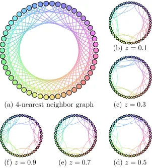
(a) 4-nearest neighbor graph (c)z= 0.3

(f)z= 0.9 (e)z= 0.7 (d)z= 0.5 (b)z= 0.1

Figure 1: The 4-nearest neighbor graph and the time-varying graph for various index values

z. The thickness of edges represents the magnitude of the inverse correlation matrix corresponding to that edge for a specific valuez.

nodes and e= 25 by selecting edge from the 4-nearest neighbor graph illustrated in Figure 1(a). We first generate Z1, . . . , Zn independently from Uniform(0,1) with the sample size

n∈ {200,500,800} and then generateΩ(z) at each index valueZi as follows.

1. Randomly select 25 edges from the 4-nearest neighbor graph and generate the initial graphG(0). The structure of the underlying graph will change at the following anchor points z = 0.2,0.4,0.6,0.8. At the `-th anchor point, we randomly remove 10 edges from the previous graphG(`−1)_{and randomly add 10 edges from the 4-nearest neighbor} graph that did not belong to the previous graph G(k−1). We therefore generate 5 anchor graphsG(0), . . . , G(4). On the`-th interval [(`−1)/5, `/5], the graph structure stays constant and equal toG(`−1) _{for`= 1, . . . ,5.}

2. Given the graph structure we generate Ω(z). At the middle of each interval, that is, for index values z= 0.1,0.3,0.5,0.7,0.9, if the edge (j, k) belongs to the graph at that time, we randomly generateΩjk(z) from Uniform[µ,0.9], whereµis the minimal

signal strength, otherwise we setΩjk(z) to be zero. For 1≤`≤4, if the edge (j, k)

belongs to both G(`) and G(`+1), we let Ωjk(z`) be generated from Uniform[µ,0.9],

otherwise we set it to be zero. We also generate Ωjk(0) from Uniform[µ,0.9] if the

edge (j, k) is in G(0) and similarly forΩjk(1) using G(4). The signal strength is set to

µ= 0.5.

3. For anyz∈(0,1), ifz∈[`/10,(`+ 1)/10] for some`= 0, . . . ,9,Ωjk(z) is set to be an

linear interpolation ofΩjk(`/10) andΩjk((`+ 1)/10). We first rescale the diagonal of

Gaussian Gaussian Copula 2% Contamination 5% Contamination

n

=

200

TPR

0.0 0.2 0.4 0.6 0.8 1.0

0.0

0.2

0.4

0.6

0.8

1.0

0.0 0.2 0.4 0.6 0.8 1.0

0.0

0.2

0.4

0.6

0.8

1.0

0.0 0.2 0.4 0.6 0.8 1.0

0.0

0.2

0.4

0.6

0.8

1.0

0.0 0.2 0.4 0.6 0.8 1.0

0.0

0.2

0.4

0.6

0.8

1.0

n

=

500

TPR

0.0 0.2 0.4 0.6 0.8 1.0

0.0

0.2

0.4

0.6

0.8

1.0

0.0 0.2 0.4 0.6 0.8 1.0

0.0

0.2

0.4

0.6

0.8

1.0

0.0 0.2 0.4 0.6 0.8 1.0

0.0

0.2

0.4

0.6

0.8

1.0

0.0 0.2 0.4 0.6 0.8 1.0

0.0

0.2

0.4

0.6

0.8

1.0

n

=

800

TPR

0.0 0.2 0.4 0.6 0.8 1.0

0.0

0.2

0.4

0.6

0.8

1.0

0.0 0.2 0.4 0.6 0.8 1.0

0.0

0.2

0.4

0.6

0.8

1.0

0.0 0.2 0.4 0.6 0.8 1.0

0.0

0.2

0.4

0.6

0.8

1.0

0.0 0.2 0.4 0.6 0.8 1.0

0.0

0.2

0.4

0.6

0.8

1.0

Kendall Pearson GLasso Neighbor

FPR FPR FPR FPR

Figure 2: ROC curves for different estimators of the inverse correlation matrix estimator. The number of nodes isd= 50, the number of edges for each index value ise= 25 and the sample size is varied in n ∈ {200,500,800}. Each curve is obtained by averaging 100 simulation runs.

ones. An illustration of the timevarying graphical model is shown in Figure 1(b) -Figure 1(f).

Given the inverse correlation matrix Ω(z), we consider four data generation schemes: 1. Gaussian, whereX |Z =z∼N(0,Σ(z));

2. Gaussian Copula, where X | Z = z ∼ (Φ(Y1(z)), . . . ,Φ(Yd(z)))T, Y | Z = z ∼

N(0,Σ(z)) and Φ(·) is the cumulative density function of standard normal distribu-tion;

3. Gaussian with 2% contamination, where X | Z = z ∼ N(0,Σ(z)) and then 2% of locations are randomly chosen and replaced by ±N(3,3);

4. Gaussian with 5% contamination, is uses the same data generating mechanism as before, but more of the observations are contaminated.

n µ0= 0 µ0= 0.4 µ0= 0.6 µ0= 0.9 600 0.108 0.722 0.892 0.994 800 0.090 0.822 0.900 0.998 1,000 0.056 0.736 0.968 1.000

Table 1: Size (bold) and power of the local edge presence test H0 :Ω12(0.5) = 0 at signif-icance level 95% with various signal strength µ0. Results reported based on 500 simulation runs.

z. The true positive rate (TPR) and false positive rate (FPR) are defined as

TPR(z) = |Eb(z)

T E∗(z)|

|E∗(z)| and FPR(z) =

|Eb(z)\E∗(z)| d(d−1)/2− |E∗(z)|,

where |S|denotes cardinality of the set S. To measure the quality of graph estimation for

z∈(0,1), we randomly choose 10 data points from{Zi}i∈[n]and compute the averaged TPR and FPR on these 10 points as the overall TPR and FPR of the graph estimation. Figure 2 illustrates the ROC curves of the overall TPR and FPR for the four competing methods under four schemes forn= 200,500 and 800. We can observe that the proposed estimator is slightly worse compared to other three estimators when the data are Gaussian conditionally on the index value. In this setting the data generating assumptions are satisfied for the other three procedures. On the other hand, when the data are generated according to the Gaussian copula distribution, the Gaussian assumption is violated and our estimator performs better compared to the other three estimators. The third and fourth columns of Figure 2 further illustrate that our estimator is more robust to corruption of data.

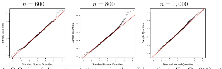
In addition to graph estimation accuracy, we consider the numerical performance of testing procedures proposed in the paper. We first focus on the local edge presence test introduced in Section 3.1. Consider the following null hypothesis H0 : Ω12(0.5) = 0. We choose the bandwidth h = 0.9n−1/5, γ = 0.5 in (3) and the penalty parameter λ = 0.2 h2₊p

log(d/h)/(nh)

for the sample size n ∈ {600,800,1000}. The data generating process is the same as before, except that we set Ω21(z) = µ0 for all z ∈ (0,1) where

µ0 ∈ {0,0.4,0.6,0.9}. We use (21) to test the null hypothesis at significance level 95% and estimate the power based on 500 repetitions. The Q-Q plots of the testing statistic

n= 600 n= 800 n= 1,000

µ= 0 µ= 0.4 µ= 0.9 µ= 0 µ= 0.4 µ= 0.9 µ= 0 µ= 0.4 µ= 0.9

k= 0 0.118 0.954 0.958 0.088 0.958 0.976 0.068 0.977 0.992

k= 2 0.128 0.900 0.926 0.090 0.944 0.964 0.070 0.970 0.982

k= 4 0.098 0.089 0.058 0.082 0.068 0.054 0.066 0.052 0.048

k= 8 0.090 0.074 0.054 0.066 0.058 0.048 0.054 0.052 0.050 Table 2: Size (bold) and power of local edge present testH0 :G∗(z)⊂G for allz ∈(0,1)

n= 600 n= 800 n= 1,000 ● ●● ● ● ● ● ● ● ● ● ● ● ● ● ●● ● ● ● ●● ● ● ● ● ●● ● ● ● ● ● ● ● ● ● ● ● ● ● ● ● ● ● ●● ● ● ● ● ● ● ● ● ● ● ● ● ● ● ● ● ● ● ● ● ● ● ● ● ● ● ● ● ● ● ● ● ● ● ● ● ● ● ● ●● ● ● ● ● ●● ● ● ● ● ● ● ● ● ● ● ● ● ● ● ● ● ● ● ● ● ● ● ● ● ● ● ● ● ● ● ● ● ● ● ● ● ● ● ●● ● ● ● ● ● ● ● ● ● ● ● ● ● ● ●● ● ● ● ● ● ● ● ● ● ● ● ● ● ● ● ● ● ● ● ● ● ● ● ● ● ● ● ● ● ● ● ●● ● ● ● ● ● ● ● ● ● ● ● ● ● ● ● ● ● ● ● ● ● ● ● ● ● ● ● ● ● ● ● ● ● ● ● ● ● ● ● ● ● ● ● ● ● ● ● ● ● ● ● ● ● ● ● ● ● ●● ● ● ● ● ● ● ● ● ● ● ● ● ● ● ● ● ● ● ●● ● ● ●● ● ● ● ● ● ● ● ● ● ● ● ● ● ● ● ● ● ● ● ● ● ● ● ● ● ● ● ● ● ● ● ● ● ● ● ● ● ● ● ● ● ● ● ● ● ● ● ● ● ● ● ● ● ●● ●●● ● ● ● ● ● ● ● ● ● ● ● ● ● ●● ● ● ● ● ● ● ● ● ● ● ● ● ● ● ● ● ● ● ● ● ● ● ● ● ●● ● ● ● ● ● ● ● ● ● ● ● ● ● ● ● ● ● ● ● ● ● ● ● ● ● ● ● ● ● ● ● ● ● ● ● ● ● ● ● ● ● ● ● ● ● ● ● ● ● ● ● ● ● ● ● ● ● ● ● ● ● ● ● ● ● ● ● ● ● ● ● ● ● ● ● ● ● ● ● ● ● ● ● ● ● ● ● ● ● ● ● ● ● ● ● ● ● ● ● ● ● ● ● ● ● ● ● ● ● ● ● ● ● ● ● ● ● ● ● ● ● ● ● ● ●● ● ● ● ● ●● ● ● ●

−3 −2 −1 0 1 2 3

−2 −1 0 1 2 3

Standard Normal Quantiles

Sample Quantiles ● ●● ● ● ● ● ● ● ● ●● ● ● ● ● ● ● ● ● ● ● ● ● ● ● ● ● ● ● ● ● ● ● ● ● ● ● ● ● ● ● ● ● ● ● ● ● ●● ● ● ● ● ● ● ● ● ● ● ● ● ● ● ● ● ● ● ● ● ● ● ● ● ● ● ● ● ● ● ● ● ● ● ● ● ● ● ● ● ● ● ● ● ● ● ● ● ● ● ●● ● ● ● ● ● ● ● ● ● ● ● ● ● ● ● ● ● ● ● ● ● ● ● ● ● ● ● ● ● ● ● ● ● ● ● ● ● ●● ● ● ● ● ● ● ● ● ● ● ● ● ● ● ● ● ● ● ● ● ● ● ● ● ● ● ● ● ● ● ● ● ● ● ● ● ● ● ● ● ● ● ● ● ● ● ● ● ● ● ● ● ● ● ●● ● ● ● ● ● ● ● ● ● ● ● ● ● ●● ● ● ● ● ● ● ● ● ● ● ● ● ● ● ● ● ● ● ● ● ● ● ● ● ● ● ● ● ● ● ● ● ● ● ● ● ● ● ● ● ● ● ● ● ● ● ● ● ● ● ● ● ● ● ● ● ● ● ● ● ● ● ● ● ● ● ● ● ● ● ● ●●●● ● ● ● ● ● ● ● ● ● ● ● ● ● ● ● ● ● ● ● ● ● ● ● ● ●● ●● ● ● ● ● ● ● ● ● ● ● ●● ● ●● ● ● ● ● ●● ● ● ● ● ● ● ● ● ● ● ● ● ● ● ● ● ● ● ● ● ● ●● ● ● ● ● ● ● ●● ● ● ● ● ● ● ● ● ● ● ● ● ● ● ● ● ● ●●● ● ● ● ● ● ●● ● ● ● ● ● ● ● ● ● ● ● ● ● ● ● ● ● ● ● ● ● ●● ● ● ● ● ● ● ● ● ● ● ● ● ● ● ● ● ● ● ● ● ● ● ● ● ● ● ● ● ● ● ● ● ● ● ● ● ● ● ● ● ● ● ● ● ● ● ● ● ● ● ● ● ● ● ● ● ● ● ● ● ● ● ● ● ● ● ● ● ● ● ● ● ● ● ● ● ● ● ● ● ● ● ●

−3 −2 −1 0 1 2 3

−2 −1 0 1 2 3

Standard Normal Quantiles

Sample Quantiles ● ● ● ● ● ● ● ● ● ● ● ●● ● ● ● ● ● ● ● ● ● ● ● ● ● ● ● ● ● ● ● ● ● ● ● ● ● ● ● ● ●● ● ● ● ● ● ● ● ● ● ● ● ● ● ● ● ● ● ● ● ● ● ● ● ●● ● ● ● ● ● ● ● ● ● ● ●● ● ● ● ● ● ● ● ● ● ● ● ● ● ● ● ● ● ● ● ● ● ● ● ● ● ● ● ● ● ● ● ● ●● ● ● ● ● ● ● ● ● ● ● ● ● ● ● ● ● ● ● ● ● ● ● ● ● ● ● ● ● ● ● ● ● ● ● ● ● ● ● ● ● ● ● ● ● ● ● ● ● ● ● ● ● ● ● ● ● ● ● ● ● ● ● ● ● ● ● ● ● ● ● ● ● ● ● ● ●● ● ● ● ● ● ● ● ● ● ● ● ● ● ● ● ● ● ● ● ● ● ● ● ● ● ● ● ● ● ●● ● ● ● ● ● ● ● ● ● ● ● ● ● ● ● ● ● ● ● ● ● ● ● ● ● ● ● ● ● ● ● ● ● ● ● ● ● ● ● ● ● ● ● ● ● ● ● ● ● ● ● ● ● ● ● ● ● ● ● ● ● ● ● ● ● ● ● ● ● ● ● ● ● ● ● ● ● ● ● ● ● ● ● ● ● ● ● ● ● ● ● ● ● ● ● ● ● ● ● ● ● ● ● ● ● ● ● ● ● ● ● ● ● ● ● ● ● ● ● ● ● ● ● ● ● ● ● ● ● ● ● ● ● ●● ● ● ● ● ● ● ● ● ● ● ● ● ● ● ● ● ● ● ● ● ● ● ● ● ● ● ● ● ● ● ● ● ● ●● ● ● ●● ● ● ● ● ● ●● ● ● ● ● ● ● ● ● ● ● ● ● ● ● ● ● ● ● ● ● ● ● ● ● ● ● ● ● ● ● ● ● ● ● ● ● ● ● ● ● ● ● ● ● ● ● ● ● ● ● ● ● ● ● ● ● ● ● ● ●● ● ● ● ● ● ●● ● ● ● ● ● ● ● ● ● ● ● ● ● ● ● ● ● ● ● ● ● ● ● ● ● ● ● ● ●

−3 −2 −1 0 1 2 3

−2 −1 0 1 2 3

Standard Normal Quantiles

Sample Quantiles

Figure 3: Q-Q plot of the testing statistic under the null hypothesis H0:Ω12(0.5) = 0.

for various sample sizes are shown in Figure 3. The empirical distribution of the testing statistic is close to standard normal distribution. The results on the power of these tests are summarized in Table 5.1. When the signal strength µ0 = 0, the size of the test approaches the nominal value 0.05. When µ ≥ 0.4, the power approaches 1, showing validity of the proposed test.

We also conduct a simulation for the uniform edge presence test introduced in Section 3.3. We consider the null hypothesis H0 : G∗(z) ⊂ G for all z ∈ (0,1), where the super graphG is ak-nearest neighbor graph for k∈ {0,2,4,8}. Here ak-nearest neighbor graph has edges only connecting a vertex to its closestknodes. See Figure 1(a) for an illustration of a 4-nearest neighbor graph. When k = 0, it is a null graph whose adjacency matrix is identity. In order to illustrate the power of our test, we generate the nonzero entries of the inverse correlation matrix at anchor points from Uniform[µ,max(µ+ 0.2,0.9)] for

µ= 0.4 and 0.9. We also consider the setting whereΩ(z) =Ifor allz∈(0,1). The sample size is varied asn∈ {600,800,1000}. The bandwidth and tuning parameter are set in the same way as for the local edge presence test. When computing the test statistic in (22) the suprema over z ∈ (0,1) is approximated by taking the maximum of the statistic over 100 evenly spaced values in (0,1), and similarly for the bootstrapped statistic in (23). The size and power of the test are summarized in Table 5.1. From the data generating mechanism, we see that the true graph is always a subgraph of the 4-nearest graph. Therefore, the null hypothesis is true when the number of nearest neighbors is k∈ {4,8} orΩ(z) =I. From the results reported in Table 5.1, we observe that the uniform edge presence test has the correct size as the sample size increases. The alternative hypothesis is true whenk∈ {0,2} and Ω(z) 6= I. In this setting, the less edges the super graph has, the more powerful the test is. That is because we take maximum over more edges in (16).

5.2 Super Brain Test

H0 :G(8)⊂G(11.75) H0:G(11.75)⊂G(20) Statistics 2.793 3.548

Quantiles 1.899 2.154

Table 3: Results on the super brain hypothesis tests at 95% significant level. The row named “Statistics” are the values of the testing statistic in (16). The row named “Quantiles” are the 95%-quantile estimators obtained by the bootstrap estimator in (19).

to the cerebral cortex and cerebellum. For each subject we also have covariates that include age, IQ, gender and handedness. For illustration purposes, we focus on 491 controls and explore how the structure of the neural network varies with age of subjects, which range from 7.08 to 21.83. Using the kernel smoothing technique to estimate the varying neural networks, Qiu et al. (2016) found that the connections tend to be denser at the age 21.83 than at ages 11.75 and 7.09. Such a discovery is also supported by Bartzokis et al. (2001) and Gelfand et al. (2003).

Based on these discoveries, a more interesting conjecture is whether the neural network is always growing with age. We can use our testing framework to investigate the claim that a neural network in a younger subject is a subgraph of a neural network in an older subject. Specifically, we choose three ages: 8, 11.75 and 20, and we are interested in the graphs

G(8),G(11.75) andG(20), whereG(z) is the true neural network at agez. The age 11.75 is chosen as the median age of subjects. We call the neural networks at ages 8, 11.75 and 20 as the junior, median and senior neural network, respectively. As we do not have access to the true networks, we will estimate them using the calibrated CLIME in (3). We first map the ages onto the interval (0,1) and set the tuning parameters for our procedure asγ = 0.5, the bandwidthh= 0.002 and the penalty parameterλ= 0.03 h2+pd/h/(nh), where the last two parameters are chosen through cross-validation. We estimate the neural networks

b

G(8),Gb(11.75) andGb(20) by (3) at ages 8, 11.75 and 20. The estimated graphs are used as

super graphs in defining the null hypothesis. In particular, we have the following two tests:

H0:G(8)⊂Gb(11.75) and H0 :G(11.75)⊂Gb(20). Although we use the random estimators

as the super graphs in these hypotheses, the testing procedure is still valid. This is because of the small bandwidthh= 0.002 making the data used in network estimation independent to the data used in these two tests. Therefore, the test can still be reduced as a super graph test.

Figure 4 shows the differences among the junior, median and senior brains. We observe that even if a later neural network has more edges compared to the earlier one, many edges existing at an earlier stage disappear later in the development. This implies that the conjecture that neural networks grow with age is not supported by the data. Table 5.2 quantifies evidence against the null hypothesis.

6. Discussion

coronal sagittal transverse

(a)Gb(8) v.s. Gb(11.75)

(b) Gb(11.75) v.s. Gb(20)

Figure 4: The differences between junior, median and senior neural networks. Gb(8),

b

G(11.75) and Gb(20) denote the estimated graphs at age 8, 11.75 and 20. The

first row is the difference between Gb(8) and Gb(11.75). The green lines are the

edges existing inGb(11.75) but not in Gb(8) and the red edges only exist in Gb(8)

but notGb(11.75). The second row is the difference betweenGb(11.75) andGb(20).

The green edges only exist inGb(20) and the red edges only exist inGb(11.75).

estimation and inference methods for the time-varying graphical model under general heavy-tailed distributions with certain moment conditions. It is possible to incorporate existing methods including the Catoni’s estimator (Catoni, 2012) and the median-of-means estima-tor (Hsu and Sabato, 2014) into the framework of this paper and conduct inference for the general heavy-tailed time-varying graphical models.

Acknowledgments