Conditional Random Field with High-order Dependencies for
Sequence Labeling and Segmentation
Nguyen Viet Cuong [email protected]
Nan Ye [email protected]
Wee Sun Lee [email protected]
Department of Computer Science National University of Singapore 13 Computing Drive
Singapore 117417
Hai Leong Chieu [email protected]
DSO National Laboratories 20 Science Park Drive Singapore 118230
Editor:Kevin Murphy
Abstract
Dependencies among neighboring labels in a sequence are important sources of informa-tion for sequence labeling and segmentainforma-tion. However, only first-order dependencies, which are dependencies between adjacent labels or segments, are commonly exploited in practice because of the high computational complexity of typical inference algorithms when longer distance dependencies are taken into account. In this paper, we give efficient inference algorithms to handle high-order dependencies between labels or segments in conditional random fields, under the assumption that the number of distinct label patterns used in the features is small. This leads to efficient learning algorithms for these conditional random fields. We show experimentally that exploiting high-order dependencies can lead to sub-stantial performance improvements for some problems, and we discuss conditions under which high-order features can be effective.
Keywords: conditional random field, semi-Markov conditional random field, high-order feature, sequence labeling, segmentation, label sparsity
1. Introduction
Many problems can be cast as the problem of labeling or segmenting a sequence of observa-tions. Examples include natural language processing tasks, such as part-of-speech tagging (Lafferty et al., 2001), phrase chunking (Sha and Pereira, 2003), named entity recognition (McCallum and Li, 2003), and tasks in bioinformatics such as gene prediction (Culotta et al., 2005) and RNA secondary structure prediction (Durbin, 1998).
Type of CRF Feature example First-order (Lafferty et al., 2001) author year Semi-CRF (Sarawagi and Cohen, 2004) author+ year+ High-order (Ye et al., 2009, this paper) author year title title High-order semi-CRF (this paper) author+ year+ title+
Table 1: Examples of the information that can be captured by different types of CRFs for the bibliography extraction task. The x+ symbol represents a segment of “1 or more” labels of classx.
givenx, and do not model the observationsx. Hence, CRFs can be used to encode complex dependencies of y on x without significantly increasing the inference and learning costs. However, inference for CRFs is NP-hard in general (Istrail, 2000), and most CRFs have been restricted to consider very local dependencies. Examples include the linear-chain CRF which considers dependencies between at most two adjacent labels (Lafferty et al., 2001) and the first-order semi-Markov CRF (semi-CRF) which considers dependencies between at most two adjacent segments (Sarawagi and Cohen, 2004), where a segment is a contiguous sequence of identical labels. In linear-chain CRF and semi-CRF, a kth-order feature is a
feature that encodes the dependency betweenxand (k+ 1) consecutive labels or segments. Existing inference algorithms for CRFs such as the Viterbi and the forward-backward algo-rithms can only handle up to first-order features, and inference algoalgo-rithms for semi-CRFs (Sarawagi and Cohen, 2004) can only handle up to first-order features between segments. These algorithms can be easily generalized to handle high-order features, but will require time exponential in k. In addition, a general inference algorithm such as the clique tree al-gorithm (Huang and Darwiche, 1996) also requires time exponential inkto handlekth-order features (k >1).
In this paper, we exploit a form of sparsity that is often observed in real data to design efficient algorithms for inference and learning with high-order label or segment dependencies. Our algorithms are presented for high-order semi-CRFs in its most general form. Algorithms for high-order CRFs are obtained by restricting the segment lengths to 1, and algorithms for linear-chain CRFs and first-order semi-CRFs are obtained by restricting the maximum order to 1.
We use a bibliography extraction task in Table 1 to show examples of features that can be used with different classes of CRFs. In this task, different fields are often arranged in a fixed order, hence using high-order features can be advantageous. The sparsity property that we exploit is the following label pattern sparsity: the number of observed sequences of k consecutive segment labels (e.g., “author+ year+ title+” is one such sequence where
algo-rithm for Viterbi parsing can also be used with cutting plane methods to train max-margin solutions for sequence labeling problems in polynomial time (Tsochantaridis et al., 2004). Our inference and learning algorithms run in time polynomial in the maximum segment length as well as the number and length of the label patterns that the features depend on. We demonstrate that modeling high-order dependencies can lead to significant perfor-mance improvements in various problems. In our first set of experiments, we focus on high-order CRFs and demonstrate that using high-order features can improve performance in sequence labeling problems. We show that in handwriting recognition, using even sim-ple high-order indicator features improves performance over using linear-chain CRFs, and significant performance improvement is observed when the maximum order of the indica-tor features is increased. We also use a synthetic data set to discuss the conditions under which high-order features can be helpful. In our second set of experiments, we demonstrate that using high-order semi-Markov features can be helpful in some applications. More specifically, we show that high-order semi-CRFs outperform high-order CRFs and first-order semi-CRFs on three segmentation tasks: relation argument detection, punctuation prediction, and bibliography extraction.1
2. Algorithms for High-order Dependencies
Our algorithms are presented for high-order semi-CRFs in its most general form. These al-gorithms generalize the alal-gorithms for linear-chain CRFs and first-order semi-CRFs, which are special cases of our algorithms when the maximum order is set to 1. They also generalize the algorithms for high-order CRFs (Ye et al., 2009), which are special cases of our algo-rithms when the segment lengths are set to 1. Thus, only the general algoalgo-rithms described in this section need to be implemented to handle all these different cases.2
2.1 High-order Semi-CRFs
Let Y ={1,2, . . . , n} denote the set of distinct labels, x = (x1, . . . , x|x|) denote an input
sequence of length|x|, andxa:b denote the sub-sequence (xa, . . . , xb). Asegment ofxis
de-fined as a triplet (u, v, y), whereyis the common label of the segmentxu:v. Asegmentation
forxa:b is a segment sequences= (s1, . . . , sp), withsj = (uj, vj, yj) such thatuj+1=vj+ 1
for all j,u1=aand vp=b. A segmentation forxa:b is a partial segmentation forx.
A semi-CRF defines a conditional distribution over all possible segmentations s of an input sequencex such that
P(s|x) = 1
Zxexp( m X
i=1 |s| X
t=1
λifi(x,s, t))
1. This paper is an extended version of a previous paper (Ye et al., 2009) published in NIPS 2009. Some of the additional material presented here has also been presented as an abstract (Nguyen et al., 2011) at the ICML Workshop on Structured Sparsity: Learning and Inference, 2011. The source code for our algorithms is available at https://github.com/nvcuong/HOSemiCRF.
2. In an earlier paper (Ye et al., 2009), we give algorithms for high-order CRFs which are similar to those presented here. The main difference lies in the backward algorithm. The version presented here is
a conditional version which uses properties of labels before the suffix labels being considered, making
where Zx=Psexp( P
i P
tλifi(x,s, t)) is the partition function with the summation over
all segmentations of x, and {fi(x,s, t)}1≤i≤m is the set of semi-Markov features, each of
which has a corresponding weight λi.
We shall work with features of the following form
fi(x,s, t) = (
gi(x, ut, vt) ifyt−|zi|+1. . . yt=zi
0 otherwise (1)
wherezi∈ Y|zi|is a segment label pattern associated with f
i, and sis a segmentation or a
partial segmentation forx. The function fi(x,s, t) depends on the t-th segment as well as
the label patternzi and is said to be of order|zi| −1. The order of the resulting semi-CRF is the maximal order of the features.
We will give exact inference algorithms for high-order semi-CRFs in the following sec-tions. As in exact inference algorithms for linear-chain CRFs and semi-CRFs, our algorithms perform forward and backward passes to obtain the necessary information for inference.
2.2 Notations
Without loss of generality, let Z ={z1, . . . ,zM} be the segment label pattern set, that is, the set of distinct segment label patterns of the m features (M ≤ m). For our forward algorithm, the forward-state set P ={p1, . . . ,p|P|} consists of distinct elements in the set of all the labels and proper prefixes (including the empty sequence ) of the segment label patterns. Thus, P =Y ∪ {zj1:k}0≤k<|zj|,1≤j≤M. For the backward algorithm, the
backward-state set S ={s1, . . . ,s|S|}consists of distinct elements inPY, that is, the set consisting of elements inP concatenated with a label in Y.
Transitions between states in our algorithm are defined using the suffix relationships between them. We use z1 ≤s z2 to denote that z1 is a suffix of z2. The longest suffix
relation on a setAis denoted byz1 ≤sAz2. This relation holds true if and only ifz1, among
all the elements of A, is the longest suffix of z2. More formally, z1 ≤sA z2 if and only if z1 ∈ Aand z1 ≤sz2 and∀z∈ A,z≤sz2 ⇒z≤sz1.
2.3 Training
Given a training setT, we estimate the model parameters~λ= (λ1, . . . , λm) by maximizing
the regularized log-likelihood function
LT(~λ) = P(x,s)∈T logP(s|x)−Pmi=1 λ2
i
2σ2 reg
whereσregis a regularization parameter. This function is convex, and thus can be maximized
using any convex optimization algorithm. In our implementation, we use the L-BFGS method (Liu and Nocedal, 1989). The method requires computation of the value of LT(~λ)
and its partial derivatives
∂LT ∂λi
= ˜E(fi)−E(fi)− λi σ2
reg
where ˜E(fi) = P
(x,s)∈T P
tfi(x,s, t) is the empirical feature sum of the feature fi, and E(fi) = P(x,s)∈T
P
s0P(s0|x)
P
tfi(x,s
0, t) is the expected feature sum of f
LT(~λ) and its partial derivatives, we need to efficiently compute the partition functionZx
and the expected feature sum of fi’s.
2.3.1 Partition Function
For any pi ∈ P, let pj,pi be the set of all segmentations for x1:j whose segment label
sequences containpi as the longest suffix among all elements inP. We define the forward variables αx(j,pi) as follows
αx(j,pi) = X
s∈pj,pi
exp(X
k X
t
λkfk(x,s, t)).
The above definition of the forward variable αx is the same as the usual definition of for-ward variable for first-order semi-CRFs when only zeroth-order and first-order semi-Markov features are used. The forward variables can be computed by dynamic programming:
αx(j,pi) =
L−1 X
d=0
X
(pk,y):pi≤s Ppky
Ψx(j−d, j,pky)αx(j−d−1,pk)
where L is the longest possible length of a segment, P
i:Pred(i) denotes summation over
all i’s satisfying the predicate Pred(i), and Ψx(u, v,p) counts the contribution of features
activated when there is a segment label sequencep with its last segment having boundary (u, v). The factor Ψx(u, v,p) is defined as
Ψx(u, v,p) = exp( X
i:zi≤sp
λigi(x, u, v)).
The correctness of the above recurrence is shown in Appendix A. The partition function can be computed from the forward variables by
Zx=X
i
αx(|x|,pi).
2.3.2 Expected Feature Sum
Letsj be the set of all partial segmentations for xj:|x|. Fors∈sj andsk∈ S, we define for
each featurefia conditional feature functionfi(x,s, t|sk), which takes the value offi(x,s, t)
when sk is the longest suffix (inS) of the segment label sequence forx1:j−1. Otherwise, its
value is 0. For example, if s= (s1, . . . , sp)∈sj and s1= (u1, v1, y1), then
fi(x,s,1|sk) = (
gi(x, u1, v1) ifzi≤ssky1
0 otherwise .
For eachsi∈ S, we define the backward variablesβx(j,si) as follows
βx(j,si) = X
s∈sj
exp(X
k X
t
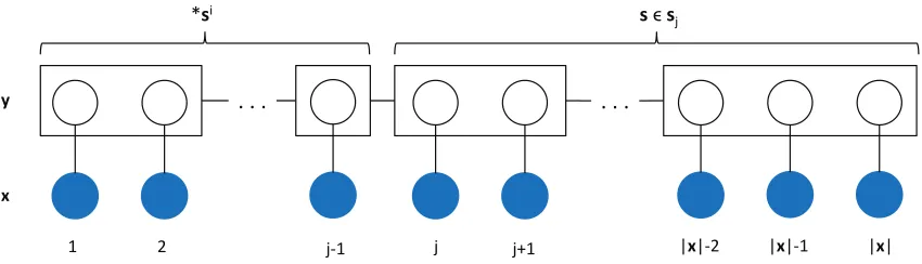
. . . . . .
j j+1
j-1
1 2 |x|-2 |x|-1 |x|
*si s s
j
x y
Figure 1: An illustration of the backward variable βx(j,si). Each rectangular box
corre-sponds to a segment. The regular expression∗si means thatsi is the suffix of the segment label sequence forx1:j−1. In fact, si is the longest suffix of the segment
label sequence forx1:j−1. The summation in the definition ofβx(j,si) is over all
the partial segmentationssof xj:|x|.
Figure 1 gives an illustration of the backward variable βx(j,si). Note that our definition of βx uses the conditional feature function and does not generalize the usual definitions of
the backward variables in first-order semi-CRFs (Sarawagi and Cohen, 2004) or high-order CRFs (Ye et al., 2009).
Similar to the case of forward variables, we can compute βx(j,si) by dynamic
program-ming:
βx(j,si) = L−1 X
d=0
X
(sk,y):sk≤s Ssiy
Ψx(j, j+d,siy)βx(j+d+ 1,sk).
In Appendix A, we show the correctness proof for the recurrence. We can now compute the marginals P(u, v,z|x) for each z∈ Z andu≤v, where P(u, v,z|x) denotes the proba-bility that a segmentation of x contains label patternz and has (u, v) as z’s last segment boundaries. These marginals can be computed by
P(u, v,z|x) = 1
Zx
X
(pi,y):z≤spiy
αx(u−1,pi)Ψx(u, v,piy)βx(v+ 1,piy).
We compute the expected feature sum for fi by
E(fi) = X
(x,s)∈T X
u≤v
P(u, v,zi|x)gi(x, u, v).
In Appendix B, we give an example to illustrate our algorithms for the second-order CRF model.
(1) only know the correct position (ut, vt) of the last segment. In other words, although
they know the label sequence of the previous segments, the features do not know the actual boundaries of these segments. So, to compute the marginal P(u, v,z|x) using the usual extension of the backward variables, we need to sum over all possible segmentations near (u, v) that contain (u, v) as a segment. This may result in an algorithm that is exponential in the order of the semi-CRFs. Note that this problem does not occur for high-order CRFs (Ye et al., 2009) since in these models, the segment length is 1 and thus we can always determine the boundaries of the segments.
2.4 Decoding
We compute the most likely segmentation for high-order semi-CRF by a Viterbi-like decod-ing algorithm. It is the same as the forward algorithm with the sum operator replaced by the max operator. Define
δx(j,pi) = max
s∈pj,pi
exp(X
k X
t
λkfk(x,s, t)).
These variables can be computed by
δx(j,pi) = max (d,pk,y):pi≤s
Ppky
Ψx(j−d, j,pky)δx(j−d−1,pk).
Note that the value ofdis inclusively between 0 andL−1 in the above equation. The most likely segmentation can be obtained using backtracking from maxiδx(|x|,pi).
2.5 Time Complexity
We now give rough time bounds for the above algorithm. It is important to note that the bounds given in this part are pessimistic, and the computation can be done more quickly in practice. For simplicity, we assume that the featuresgi(·,·,·) can be computed inO(1) time
for all i ∈ {1,2, . . . , m} and the algorithm would pre-compute all the values of Ψx before
doing the forward and backward passes. This assumption often holds for features used in practice, although one can define gi’s which are arbitrarily difficult to compute.
Since the total number of different patterns of the last argument of Ψx is O(|S||Y|) = O(|P||Y|2), the time complexity to pre-compute all the values of Ψ
x in the worst case is O(mT2|P||Y|2) = O(mn2T2|P|), where T is the maximum length of an input sequence.
After pre-computing the values of Ψx, we can compute all the values of αx inO(T2|Y||P|)
time. Similarly, the time complexity to compute all the values of βx isO(T2|Y||S|). Then,
with these values, we can compute all the marginal probabilities in O(T2|Z||P|). Finally, the time complexity for decoding is O(T2|Y||P|).
3. Experiments
3.1 Experiments with High-order CRFs
The practical feasibility of making use of high-order features based on our algorithm lies in the observation that the label pattern sparsity assumption often holds. Our algorithm can be applied to take those high-order features into consideration: high-order features now form a component that one can play with in feature engineering.
Now, the question is whether high-order features arepractically significant. We first use a synthetic data set to explore conditions under which high-order features can be expected to help. We then use a handwritten character recognition problem to demonstrate that even incorporating simple high-order features can lead to impressive performance improvement on a naturally occurring data set.3
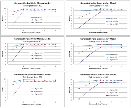
3.1.1 Synthetic Data Generated Using kth-order Markov Model
We randomly generate an order k Markov model with n states s1, . . . , sn as follows. To
increase pattern sparsity, we allow at mostrrandomly chosen possible next states given the previouskstates. This limits the number of possible label sequences in each length (k+ 1) segment fromnk+1 tonkr. The conditional probabilities of thesernext states are generated by randomly selecting a vector from the uniform distribution over [0,1]r and normalizing
them. Each state si generates an observation (a1, . . . , am) such that aj follows a Gaussian
distribution with mean µij and standard deviationσ. Each µi,j is independently randomly
generated from the uniform distribution over [0,1]. In the experiments, we use values of
n= 5, r= 2 and m= 3.
The standard deviation σ controls how much information the observations reveal about the states. If σ is very small as compared to most µij’s, then using the observations alone
as features is likely to be good enough to obtain a good classifier of the states; the label correlations become less important for classification. However, if σ is large, then it is difficult to distinguish the states based on the observations alone and the label correlations, particularly those captured by higher order features are likely to be helpful.
We use the current, previous, and next observations, rather than just the current obser-vation as features, exploiting the conditional probability modeling strength of CRFs. For higher order features, we simply use all indicator features that appeared in the training data up to a maximum order. We considered the case k= 2 and k= 3, and varied σ and the maximum order. We run the experiment with training sets that contain 300, 400, and 500 sequences, and evaluate the models on a test set that contains 500 sequences. All the sequences are of length 20; each sequence was initialized with a random sequence of length
k and generated using the randomly generated orderk Markov model. Training was done by maximizing the regularized log-likelihood with regularization parameter σreg = 1 in all
experiments in this paper. The experimental results are shown in Figures 2.
Figure 2 shows that the high-order indicator features are useful in all cases. In particular, we can see that it is beneficial to increase the order of the high-order features when the underlying model has longer distance correlations. As expected, increasing the order of the features beyond the order of the underlying model is not helpful. The results also suggest
86 88 90 92 94 96 98 100
1 2 3 4 5
A
cc
u
ra
cy
Maximum Order of Features Generated by 2nd-Order Markov Model
Training set size = 300
Sigma=0.01 Sigma=0.05 Sigma=0.10 83 85 87 89 91 93 95 97 99
1 2 3 4 5
A
cc
u
ra
cy
Maximum Order of Features
Generated by 3rd-Order Markov Model
Training set size = 300
Sigma=0.01 Sigma=0.05 Sigma=0.10 86 88 90 92 94 96 98 100
1 2 3 4 5
A
cc
u
ra
cy
Maximum Order of Features Generated by 2nd-Order Markov Model
Training set size = 400
Sigma=0.01 Sigma=0.05 Sigma=0.10 83 85 87 89 91 93 95 97 99
1 2 3 4 5
A
cc
u
ra
cy
Maximum Order of Features Generated by 3rd-Order Markov Model
Training set size = 400
Sigma=0.01 Sigma=0.05 Sigma=0.10 86 88 90 92 94 96 98 100
1 2 3 4 5
A
cc
u
ra
cy
Maximum Order of Features Generated by 2nd-Order Markov Model
Training set size = 500
Sigma=0.01 Sigma=0.05 Sigma=0.10 83 85 87 89 91 93 95 97 99
1 2 3 4 5
A
cc
u
ra
cy
Maximum Order of Features Generated by 3rd-Order Markov Model
Training set size = 500
Sigma=0.01 Sigma=0.05 Sigma=0.10
Figure 2: Accuracy of high-order CRFs as a function of maximum order on synthetic data sets.
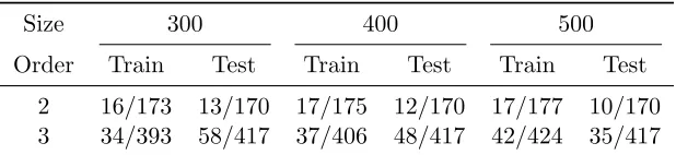
Size 300 400 500
Order Train Test Train Test Train Test
2 16/173 13/170 17/175 12/170 17/177 10/170
3 34/393 58/417 37/406 48/417 42/424 35/417
Table 2: Proportions of length 5 patterns exclusive to training and test data where the data sets are generated by 2nd-order and 3rd-order Markov models. For each proportion,
the denominator shows the number of patterns in the data set, and the numerator shows the number of patterns exclusive to it. Nearly all of these patterns occur for less than 5 times (mostly once or twice). Note that the labels are first generated independently ofσin our data sets, thus the statistics are the same for allσvalues.
In practical problems, regularization may work well as a means for avoiding overfitting spurious high-order features. But this depends on how heavily the training process is regularized, and some tuning may be needed. For example, for a regularizer like Gaussian regularizerP
i λ2
i
2σ2
reg, the parameterσreg is often determined using a validation data set or
cross-validation on the training data.
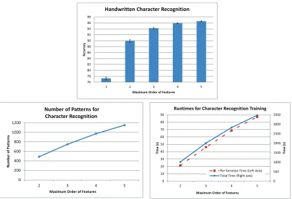
3.1.2 Handwriting Recognition
We used the handwriting recognition data set (Taskar et al., 2004), consisting of around 6100 handwritten words with an average length of around 8 characters. The data was originally collected by Kassel (1995) from around 150 human subjects. The words were segmented into characters, and each character was converted into an image of 16 by 8 binary pixels. In this labeling problem, each xi is the image of a character, and each yi is a lower-case
letter. The experimental setup is the same as that used by Taskar et al. (2004): the data set was divided into 10 folds with each fold having approximately 600 training and 5500 test examples and the zero-th order features for a character are the pixel values.
For high-order features, we again used all indicator features that appeared in the training data up to a maximum order. The average accuracies over the 10 folds are shown in Figure 3, where strong improvements are observed as the maximum order increases. Figure 3 also shows the number of label patterns, the total training time, and the running time per iteration of the L-BFGS algorithm (which requires computation of the gradient and value of the function at each iteration). Both the number of patterns and the running time appear to grow no more than linearly with the maximum order of the features for this data set.
3.2 Experiments with High-order Semi-CRFs
76 78 80 82 84 86 88 90 92 94 96 98
1 2 3 4 5
A
cc
u
rac
y
Maximum Order of Features Handwritten Character Recognition
0 200 400 600 800 1000 1200
2 3 4 5
N u mb e r o f P a tte rn s
Maximum Order of Features Number of Patterns for
Character Recognition 0 500 1000 1500 2000 2500 3000 3500 0 10 20 30 40 50 60 70 80 90
2 3 4 5
T im e ( s) T im e ( s)
Maximum Order of Features
Runtimes for Character Recognition Training
Per Iteration Time (Left Axis) Total Time (Right axis)
Figure 3: Accuracy (top), number of label patterns (bottom left), and running time (bottom right) as a function of maximum order for the handwriting recognition data set.
refer to kth-order CRF and semi-CRF respectively. We also give the number of segment label patterns and the running time of high-order semi-CRFs on the tasks.
To test if the results obtained by high-order semi-CRFs are significantly better than lower order ones in terms of F1-measure, we perform the randomization tests described by Noreen (1989) and Yeh (2000). In such tests, we shuffle the responses by randomly reassigning the outputs of two systems we are comparing, and see how likely such a shuffle produces a difference in the metric of interest (in our case, the F1-measure). An exact randomization test will iterate through all possible shuffles, but due to the large data sizes, we use an approximate randomization test where for each comparison, we perform 10000 random shuffles, and we repeat this for 999 times. It can be shown (Noreen, 1989; Yeh, 2000) that the significance levelpis at mostp0= (nc+ 1)/(nt+ 1), wherencis the number of trials
in which the difference between the F1-measures is greater than the original difference, and
nt is the total number of iterations (in our case, 999). In Table 4, 7, and 9, we summarize
3.2.1 Relation Argument Detection
In this experiment, we consider the problem of relation argument detection, which identifies and labels arguments of relations in English sentences. More specifically, we construct the label sequence for each sentence as follows: If a word in a sentence is the first argument of a relation, we label it asArg1. If it is the second argument, we label it asArg2. If the word is the first argument of a relation and it is also the second argument of another relation of the same type, we label it as Arg1Arg2. Otherwise, we label it as O, which means the word is not part of any relation. For example, in the labeled sentence “Peter/Arg1 is/O working/O for/O IBM/Arg2 ./O”, Peter and IBM are arguments of a relation.
It is important to note that if a sentence contains many Arg1’s and Arg2’s, we do not know which pairs of Arg1 and Arg2 would be the actual arguments of a relation. Furthermore, the matching of Arg1’s and Arg2’s is not one-to-one either, since a word may participate in many different relations of the same type. Thus, to actually extract the relations in a sentence, we would need a separate classifier to determine which pairs ofArg1 and Arg2 are the true mentions of a relation. In this experiment, however, we only focus and report on the sentence labeling task.
The relation argument detection problem can be thought of as part of the relation extraction task, which requires extracting some prespecified relationships between named entity mentions. For example, if a person works for an organization, then the person and the organization form an organization-affiliation relation. Previous works on the relation extraction problem usually involve building a classifier to decide whether two named entity mentions are the actual arguments of the relation (GuoDong et al., 2005; Zhang et al., 2006). It may also be beneficial for the classifiers if they can make use of the information obtained from relation argument detection.
We compared the models on the English portion of the Automatic Content Extraction (ACE) 2005 corpus (Walker et al., 2006). The corpus contains articles from six source domains and we group the labeled relations into six types. For the experiment, we trained a separate tagger for each type of relations. The training set contains 70% of the sentences from each source domain. The remaining 30% of the sentences are used for testing. Most sentences do not contain a relation and they make the trained tagger less likely to predict an argument. Hence, we randomly sampled from these negative examples so that the numbers of positive and negative examples are the same. We also assumed the manually annotated named entity mentions are known.
For linear-chain CRF, the zeroth-order features are: surrounding words before and after the current word and their capitalization patterns; letter n-grams in words; surrounding named entity mentions, part-of-speeches before and after the current word and their com-binations. The first-order features are: transitions without any observation, transitions with the current or previous words or combinations of their capitalization patterns. The high-order CRFs and CRFs include additional high-order Markov and high-order semi-Markov transition features.
Type C1 C2 C3 SC1 SC2 SC3 Part-Whole 38.68 41.41 46.52 38.57 42.56 44.30
Phys 33.24 33.60 35.20 33.35 42.04 42.46 Org-Aff 60.56 63.28 64.93 60.77 63.72 64.86 Gen-Aff 31.00 35.84 40.16 31.19 35.85 38.09 Per-Soc 53.67 58.62 58.31 53.46 57.66 57.07 Art 40.30 43.80 46.35 40.61 49.21 48.78 Average 42.91 46.09 48.58 42.99 48.51 49.26
Table 3: F1 scores of different CRF taggers for relation argument detection on six types of relations.
C2 C3 SC1 SC2 SC3
C1 0.001< 0.001<
0.226< 0.001< 0.001<
C2
– 0.001< 0.001> 0.001< 0.001<
C3
– – 0.001> 0.441> 0.074<
SC1 – – – 0.001< 0.001<
SC2 – – – – 0.017<
Table 4: The values ofp0 obtained in the statistical significance tests comparing CRFs and semi-CRFs of different orders in the relation argument detection task, where the
p-value of the significance test is smaller than p0. Figures in bold are where the difference is statistically significant at the 1% confidence level. The symbol <
(respectively>) at position (i, j) means that the system on row iperforms worse (respectively better) than the system on columnj.
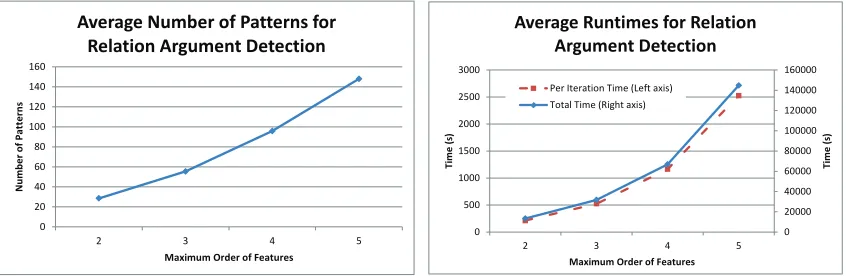
for this task, first-order semi-CRF does not perform significantly better than simple linear-chain CRF. We also observe that SC3 outperforms C1, C2, and SC1 significantly, while it outperformsC3 andSC2 withp-values at most 7.4% and 1.7% respectively. Figure 4 shows the average number of segment label patterns and the average running time of high-order semi-CRFs as a function of the maximum order.
The CRFs in Table 3 do not use begin-inside-outside (BIO) encoding of the labels. In the labeling protocol described above for this problem, although the label O indicates the outside of any argument, we do not differentiate between the beginning and the insides of an argument. In Table 5, we report the F1 scores of C1,C2, and C3 using BIO encoding (C1-BIO, C2-BIO, andC3-BIO respectively). We useArg1-B,Arg2-B, and Arg1Arg2-B to indicate the beginning of an argument and useArg1-I,Arg2-I, and Arg1Arg2-I to indicate the insides of an argument. The scores are computed after removing the B and I suffixes in the labels. From the results in Table 5, BIO encoding does not help C1-BIO and C2 -BIO much, but it helps to improve C3-BIO substantially. Overall, C3-BIO achieves the best average F1 score (51.11%) for the relation argument detection problem. Comparing
0 20 40 60 80 100 120 140 160
2 3 4 5
N
u
m
b
e
r
o
f
P
at
te
rn
s
Maximum Order of Features Average Number of Patterns for
Relation Argument Detection
0 20000 40000 60000 80000 100000 120000 140000 160000
0 500 1000 1500 2000 2500 3000
2 3 4 5
T
im
e
(
s)
T
im
e
(
s)
Maximum Order of Features
Average Runtimes for Relation Argument Detection
Per Iteration Time (Left axis)
Total Time (Right axis)
Figure 4: Average number of segment label patterns (left) and average running time (right) of high-order semi-CRFs as a function of maximum order for relation argument detection.
Type C1 C2 C3 SC3 C1-BIO C2-BIO C3-BIO Part-Whole 38.68 41.41 46.52 44.30 38.66 41.23 50.30
Phys 33.24 33.60 35.20 42.46 33.81 34.77 36.88 Org-Aff 60.56 63.28 64.93 64.86 61.33 64.33 67.50 Gen-Aff 31.00 35.84 40.16 38.09 30.38 35.03 43.37 Per-Soc 53.67 58.62 58.31 57.07 55.07 58.50 59.37 Art 40.30 43.80 46.35 48.78 40.62 43.01 49.25 Average 42.91 46.09 48.58 49.26 43.31 46.15 51.11
Table 5: F1 scores of different (non-semi) CRF taggers for relation argument detection using BIO encoding of the labels (C1-BIO,C2-BIO, andC3-BIO). The scores ofC1,C2,
C3, and SC3 are copied from Table 3 for comparison.
the arguments are located further apart. C3-BIO, on the other hand, is useful for other relations where the arguments are located near to each other.
3.2.2 Punctuation Prediction
Tag C1 C2 C3 SC1 SC2 SC3
Comma 59.29 59.70 59.90 61.13 60.89 60.35
Period 75.37 75.37 75.46 75.03 78.97 78.82
QMark 58.18 59.54 60.57 57.61 74.05 73.56
All 66.21 66.53 66.85 66.73 70.85 70.47
Table 6: F1 scores for punctuation prediction task. The last row contains the micro-averaged scores.
C2 C3 SC1 SC2 SC3
C1
0.155< 0.048< 0.043< 0.001< 0.001<
C2
– 0.153< 0.289< 0.001< 0.001<
C3
– – 0.378> 0.001< 0.001<
SC1
– – – 0.001< 0.001<
SC2
– – – – 0.044>
Table 7: The values ofp0 obtained in the statistical significance tests comparing CRFs and semi-CRFs of different orders in the punctuation prediction task, where thep-value of the significance test is smaller than p0. Figures in bold are where the difference is statistically significant at the 1% confidence level. The symbol< (respectively
>) at position (i, j) means that the system on rowiperforms worse (respectively better) than the system on column j.
60% of the texts for training and the remaining 40% for testing. The punctuation and case information are removed, and the words are tagged with different labels.
Originally, there are 4 labels: None, Comma, Period, and QMark, which respectively indicate that no punctuation, a comma, a period, or a question mark comes immediately after the current word. To help capture the long-range dependencies, we added 6 more labels: None-Comma, None-Period, None-QMark, Comma-Comma, QMark-QMark, and Period-Period. The left parts of these labels serve the same purpose as the original four labels. The right parts of the labels indicate that the current word is the beginning of a text segment which ends in comma, period, or question mark. This part is used to capture useful information at the beginning of the segment. For example, the sentence “no, she is working.” would be labeled as “no/Comma-Comma she/None-Period is/None working/Period”. In this case, she is working is a text segment (with length 3) that ends with a period. This information is marked in the label of the word working and the right part of the label of the word she. The text segment no (with length 1) is also labeled in a similar way.
0 200 400 600 800 1000 1200 1400 1600
2 3 4 5
N u m b e r o f P at t e r n s
Maximum Order of Features Number of Patterns for
Punctuation Prediction 0 20000 40000 60000 80000 100000 120000 0 200 400 600 800 1000 1200 1400 1600 1800 2000
2 3 4 5
T im e ( s) T im e ( s)
Maximum Order of Features
Runtimes for Punctuation Prediction
Per Iteration Time (Left axis)
Total Time (Right axis)
Figure 5: Number of segment label patterns (left) and running time (right) of high-order semi-CRFs as a function of maximum order for the punctuation prediction data set.
SCk uses kth-order semi-Markov transition features with the observed words in the last segment.
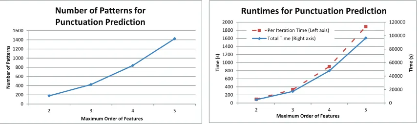
The scores reported in Table 6 are lower than those of the IWSLT corpus (Lu and Ng, 2010) because online movie transcripts are usually annotated by different people, and they tend to put the punctuations slightly differently. Besides, in movies, people sometimes use declarative sentences as questions. Hence, the punctuations are harder to predict. Never-theless, the results have clearly shown that high-order semi-CRFs can capture long-range dependencies with the help of additional labels and can achieve more than 3.6% improve-ment in F1 score compared to the CRFs and first-order semi-CRF. SCk also outperforms Ckfor allk. For this task, using third-order semi-Markov features decrease the performance of SC3 slightly compared to SC2. From Table 7, we see that thep-value of the statistical significance test comparingSC2 and SC3 is at most 4.4%, while bothSC2 and SC3 signif-icantly outperform the other models. Figure 5 shows the number of segment label patterns and the running time of high-order semi-CRFs as a function of the maximum order.
3.2.3 Bibliography Extraction
In this experiment, we consider the problem of bibliography extraction in scientific papers. For this problem, we need to divide a reference, such as those appearing in the References section of this paper, into the following 13 types of segments: Author, Booktitle, Date, Editor, Institution, Journal, Location, Note, Pages, Publisher, Tech, Title, or Volume. The problem can be naturally considered as a sequence labeling problem with the above labels. We evaluated the performance of high-order semi-CRFs and CRFs on the bibliography extraction problem with the Cora Information Extraction data set.4 In the data set, there
are 500 instances of references. We used 300 instances for training and the remaining 200 instances for testing.
We reported in Table 8 the F1 scores of the models. InC1, zeroth-order features include the surrounding words at each position and letter n-grams, and first-order features include
Tag C1 C2 C3 SC1 SC2 SC3 Author 94.21 91.65 93.67 93.97 94.74 94.00 Booktitle 73.05 75.00 72.39 75.74 78.11 76.47 Date 95.67 96.68 94.36 95.19 95.43 95.70 Editor 68.57 72.73 66.67 57.14 58.82 54.55 Institution 68.57 64.71 64.71 70.27 70.27 64.86 Journal 78.08 78.32 78.32 77.55 77.55 75.68 Location 70.33 69.66 68.13 68.13 67.39 65.22
Note 66.67 57.14 57.14 57.14 66.67 66.67
Pages 84.82 87.83 85.34 85.96 86.96 87.18 Publisher 84.62 84.62 83.54 84.62 86.08 86.08 Tech 77.78 80.00 80.00 77.78 77.78 77.78 Title 89.62 85.42 86.73 90.18 92.23 90.95 Volume 66.23 75.68 72.60 71.90 72.37 75.00 All 85.34 85.47 84.77 85.67 86.67 86.07
Table 8: F1 scores for bibliography extraction task. The last row contains the micro-averaged scores.
C2 C3 SC1 SC2 SC3
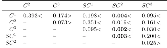
C1 0.393< 0.174> 0.198< 0.004< 0.095< C2 – 0.073> 0.351< 0.019< 0.161< C3 – – 0.095< 0.002< 0.030<
SC1
– – – 0.003< 0.200<
SC2
– – – – 0.025>
Table 9: The values ofp0 obtained in the statistical significance tests comparing CRFs and semi-CRFs of different orders in the bibliography extraction task, where the p -value of the significance test is smaller than p0. Figures in bold are where the difference is statistically significant at the 1% confidence level. The symbol <
(respectively>) at position (i, j) means that the system on row iperforms worse (respectively better) than the system on columnj.
transitions with words at the current or previous positions. Ck and SCk (1≤k≤ 3) use additionalkth-order Markov and semi-Markov transition features.
0 100 200 300 400 500 600 700
2 3 4 5
N u m b e r o f P at te rn s
Maximum Order of Features
Number of Patterns for Bibliography Extraction 0 22000 44000 66000 88000 110000 132000 154000 176000 198000 220000 500 1000 1500 2000 2500 3000 3500 4000 4500 5000 5500
2 3 4 5
T im e ( s) T im e ( s)
Maximum Order of Features
Runtimes for Bibliography Extraction
Per Iteration Time (Left axis) Total Time (Right axis)
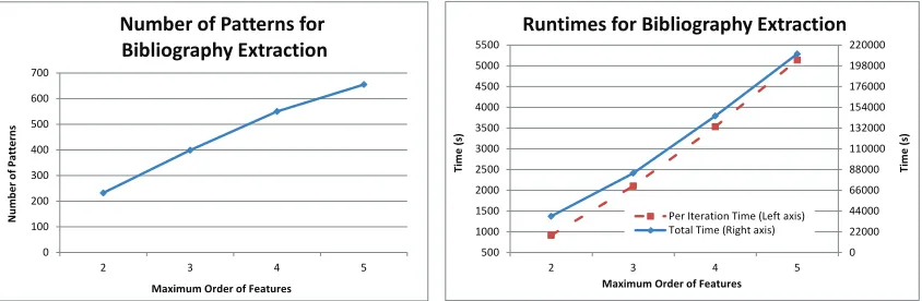
Figure 6: Number of segment label patterns (left) and running time (right) of high-order semi-CRFs as a function of maximum order for the bibliography extraction data set.
3.3 Discussions
From Figures 4, 5, and 6, the number of segment label patterns of high-order features grows about linearly in the maximum order of features. The running time of high-order semi-CRFs on the bibliography extraction task is also nearly linear in the maximum order of the features, while the running times on the relation argument detection task and the punctuation prediction task grow more than linearly in the maximum order of features. We also note that from the time complexity discussions in Section 2.5 and the setup for these experiments, the time complexity of our algorithm is O(|Z|2), where |Z| is the number of
segment label patterns.
From Tables 6 and 8, there is a drop in F1 scores for the punctuation prediction task and the bibliography extraction task when we increase the order of the semi-CRFs from 2 to 3. For the punctuation task, the drop is not very significant and the third-order semi-CRF still performs significantly better than the CRFs or the first-order semi-CRFs. For the bibliography extraction task, there is a big drop in the F1 scores for some of the labels and the third-order semi-CRF does not significantly outperform the other models. However, it does not indicate that the third-order semi-CRF is not useful for this task since we fixed the regularization parameter σreg = 1 for all the models in this experiment. If we
setσreg= 10 for the third-order semi-CRF, it can achieve 87.45% F1 score and outperform
all the other models. In practice, if we have enough data, we can choose a suitableσreg for
each individual model using a validation data set or cross-validation on the training data. We can also allow different regularizers for features of different orders5 and use a validation set to determine the most suitable combination of regularizers.
An important question in practice is which features (or equivalently, label patterns) should be included in the model. In our experiments, we used all the label patterns that appear in the training data. This simple approach is usually reasonable with a suitable value of the regularization parameter σreg. For applications where the pattern sparsity
assumption is not satisfied, but certain patterns do not appear frequently enough and are
not really important, then it is useful to see how we can select a subset of features with few distinct label patterns automatically. One possible approach would be to use boosting type methods (Dietterich et al., 2004) to sequentially select useful features.
For high-order CRFs, it should be possible to use kernels within the approach here. On the handwritten character problem, Taskar et al. (2004) reported substantial improvement in performance with the use of kernels. Use of kernels together with high-order features may lead to further improvements. However, we note that the advantage of the higher order features may become less substantial as the observations become more powerful in distinguishing the classes. Whether the use of higher order features together with kernels brings substantial improvement in performance is likely to be problem dependent.
4. Related Work
A commonly used inference algorithm for CRFs is the clique tree algorithm (Huang and Darwiche, 1996). Defining a feature depending on k (not necessarily consecutive) labels will require forming a clique of sizek, resulting in a clique-tree with tree-width greater or equal to k. Inference on such a clique tree will be exponential ink. For sequence models, a feature of order k can be incorporated into a kth-order Markov chain, but the complexity of inference is again exponential in k. Under the label pattern sparsity assumption, our algorithm achieves efficiency by maintaining only information related to a few occurred patterns, while previous algorithms maintain information about all (exponentially many) possible patterns.
Long distance dependencies can also be captured using hierarchical models such as Hierarchical Hidden Markov Model (HHMM) (Fine et al., 1998) or Probabilistic Context Free Grammar (PCFG) (Heemskerk, 1993). The time complexity of inference in an HHMM isO(min{nl3, n2l}) (Fine et al., 1998; Murphy and Paskin, 2002), wherenis the number of states andlis the length of the sequence. Discriminative versions such as hierarchical semi-CRF have also been studied (Truyen et al., 2008). Inference in PCFG and its discriminative version can also be efficiently done in O(ml3) where m is the number of productions in the grammar (Jelinek et al., 1992). These methods are able to capture dependencies of arbitrary lengths, unlike kth-order Markov chains. However, to do efficient learning with these methods, the hierarchical structure of the examples needs to be provided. For example, if we use PCFG to do character sequence labeling, we need to provide the parse trees for efficient learning; providing the labels for each character is not sufficient. Hence, a training set that has not been labeled with hierarchical labels will need to be relabeled before it can be trained efficiently. Alternatively, methods that employ hidden variables can be used (e.g., to infer the hidden parse tree) but the optimization problem is no longer convex and local optima can sometimes be a problem. The high-order semi-CRF presented in this paper allows us to capture a different class of dependencies that does not depend on hierarchical structures in the data, while keeping the high-order semi-CRF objective a convex optimization problem.
(2012) developed an efficient decoding algorithm under the assumption that all the high-order features have non-negative weights. Their decoding algorithm requires quadratic running time on the number of high-order features in the worst case.
There are other models similar to the high-order CRF with pattern sparsity assumption (Ye et al., 2009), a special case of the high-order semi-CRF presented in this paper. They include the CRFs that use the sparse higher-order potentials (Rother et al., 2009) or the pattern-based potentials (Komodakis and Paragios, 2009). Rother et al. (2009) proposed a method for minimization of sparse higher order energy functions by first transforming them into a quadratic functions and then employing efficient inference algorithms to minimize these resulting functions. For the pattern-based potentials, Komodakis and Paragios (2009) derived an efficient message-passing algorithm for inference. The algorithm is based on the master-slave framework where the original high-order optimization problem is decomposed into smaller subproblems that can be solved easily. Other tractable inference algorithms with high-order potentials include the α-expansion and αβ-swap algorithms for the Pn
Potts model (Kohli et al., 2007) and the MAP message passing algorithm for cardinality and order potentials (Tarlow et al., 2010). A special case of the order potentials, the before-after potential (Tarlow et al., 2010), can also be used to capture some semi-Markov structures in the data labelings.
5. Conclusion
The label pattern sparsity assumption often holds in real applications, and we give efficient inference algorithms for CRFs using high-order dependencies between labels or segments when the pattern sparsity assumption is satisfied. This allows high-order features to be explored in feature engineering for real applications. We studied the conditions that are favorable for using high-order features in CRFs with a synthetic data set, and demonstrated that using simple high-order features can lead to performance improvement on a handwriting recognition problem. We also demonstrated that order semi-CRFs outperform high-order CRFs and first-high-order semi-CRF in segmentation problems like relation argument detection, punctuation prediction, and bibliography extraction.
Acknowledgments
Appendix A. Correctness of the Forward and Backward Algorithms
In this appendix, we will prove the correctness of the forward and backward algorithms described in Section 2. We shall prove two lemmas and then provide the proofs for the correctness of the forward and backward algorithms as well as the marginal computation.
Lemma 1 below gives the key properties that can be used in an inductive proof. Lemma 1(a) shows that we can partition the segmentations using the forward states. Lemma 1(b-c) show that considering all (pk, y) : pi ≤s
P pky is sufficient for obtaining the sum over
all sequences pi ≤s
P zy, while Lemma 1(d) is used to show that the features are counted
correctly.
Lemma 1 Let s be a segmentation for a prefix of x. Letω(s, t) = exp(Pmk=1λkfk(x,s, t))
and ω(s) = exp(Pmk=1P|s|
t=1λkfk(x,s, t)) =Q |s|
t=1ω(s, t).
(a) For any segment label sequence z, there exists a unique pi ∈ P such that pi ≤s P z.
(b) For any segment label sequence zandy∈ Y, if pk ≤s
P z andpi≤sP pky, thenpi ≤sP zy.
(c) For any za ∈ Z, y ∈ Y, and any segment label sequence z, if za ≤s zy, and pk ≤s P z,
thenza≤spky.
(d) Lets= ((u1, v1, y1), . . . ,(u|s|, v|s|, y|s|))and letpkt ≤sP y1y2. . . ytfort= 1, . . . ,|s|. Then ω(s) =Q|s|
t=1Ψx(ut, vt,pkt−1yt) =ω(s1:|s|−1)Ψx(u|s|, v|s|,pk|s|−1y|s|). A.1 Proof of Lemma 1
(a) The intersection of P and the set of prefixes ofz contains at least one element , and is finite.
(b) We havepi≤spky≤szy. Furthermore, ifpj ≤szy, then we havepj
1:|pj|−1 ≤sz. Thus,
pj1:|pj|−1 ≤s pk since pk ≤sP z. Hence, pj =p j
1:|pj|−1y ≤s pky. Sincepi ≤sP pky, we
have pj ≤spi. Therefore,pi≤s P zy.
(c) Since za
1:|za|−1 ≤sz and pk≤sP z, we havez1:a|za|−1≤spk. Thus, za≤s pky.
(d) Straightforward from part (c) and definition of Ψx.
Lemma 2 below serves the same purpose as Lemma 1 for showing correctness.
Lemma 2 Letsbe a segmentation for a suffix ofx. Letω(s, t|si) = exp(Pmk=1λkfk(x,s, t|si))
and ω(s|si) = exp(Pmk=1P|s|
t=1λkfk(x,s, t|si)) =Q |s|
t=1ω(s, t|si).
(a) For all si ∈ S and y∈ Y, there exists a uniquesk∈ S such that sk≤s S siy.
(b) For any za ∈ Z and any segment label sequences z1,z2, if za ≤s z1z2, and si ≤sS z1,
thenza≤ssiz 2.
(c) If sk ≤s
S siy, and (u, v, y)·s is a segmentation for xu:|x|, then ω((u, v, y) ·s|si) =
Ψx(u, v,siy)ω(s|sk).
A.2 Proof of Lemma 2
(b) This is clearly true if za is not longer than z2. If za is longer than z2, let p be the
prefix ofzaobtained by stripping off the suffixz2. Thenpis a suffix ofz1 andp∈ S.
Since si is the longest suffix ofz1 inS,p is a suffix ofsi, thusza =pz2 is a suffix of siz2.
(c) From part (b), we haveω(s|siy) =ω(s|sk). Thus,ω((u, v, y)·s|si) = Ψx(u, v,siy)ω(s|siy) =
Ψx(u, v,siy)ω(s|sk).
A.3 Correctness of the Forward Algorithm
Given the forward variables αx(j,pi) as defined in Section 2
αx(j,pi) = X
s∈pj,pi
exp( m X k=1 |s| X t=1
λkfk(x,s, t)) = X
s∈pj,pi
ω(s),
we prove that the following recurrence can be used to computeαx(j,pi)’s by induction on
j,
αx(j,pi) = L−1 X
d=0
X
(pk,y):pi≤s Ppky
Ψx(j−d, j,pky)αx(j−d−1,pk). (2)
Base case: If j= 1, for anypi∈ P, we can initialize the values ofαx(1,pi) such that
αx(1,pi) = X
s∈p1,pi
exp( m X k=1 |s| X t=1
λkfk(x,s, t)) = X
s∈p1,pi
ω(s).
Inductive step: Assume that for all j0 < j and pi ∈ P, we have
αx(j0,pi) = X
s∈pj0,pi
exp( m X k=1 |s| X t=1
λkfk(x,s, t)) = X
s∈pj0,pi
ω(s).
Then, using Lemma 1,
αx(j,pi) = Ps∈pj,piω(s)
= PLd=0−1P
(pk,y):pi≤s Ppky
P
s∈pj−d−
1,pkω(s
·(j−d, j, y))
= PLd=0−1P
(pk,y):pi≤s Ppky
P
s∈pj−d−
1,pk[Ψx(j
−d, j,pky)Q|s|
t=1ω(s, t)]
= PLd=0−1P
(pk,y):pi≤s
PpkyΨx(j−d, j,p
ky)P
s∈pj−d−1,pk
Q|s|
t=1ω(s, t)
= PLd=0−1P
(pk,y):pi≤s
PpkyΨx(j−d, j,p
ky)αx(j−d−1,pk).
A.4 Correctness of the Backward Algorithm
Given the backward variables βx(j,si) as defined in Section 2
βx(j,si) = X s∈sj exp( m X k=1 |s| X t=1
λkfk(x,s, t|si)) = X
s∈sj
ω(s|si),
we prove that the following recurrence can be used to compute βx(j,si)’s by induction on j,
βx(j,si) =
L−1 X
d=0
X
(sk,y):sk≤s Ssiy
Ψx(j, j+d,siy)βx(j+d+ 1,sk). (3)
Base case: Ifj=|x|, for anysi∈ S, we can initialize the values ofβx(|x|,si) such that
βx(|x|,si) = X
s∈s|x|
exp( m X k=1 |s| X t=1
λkfk(x,s, t|si)) = X
s∈s|x|
ω(s|si).
Inductive step: Assume that for all j0 > j and si ∈ S, we have
βx(j0,si) = X
s∈sj0
exp( m X k=1 |s| X t=1
λkfk(x,s, t|si)) = X
s∈sj0
ω(s|si).
Then, using Lemma 2,
βx(j,si) = Ps∈sjω(s|s
i)
= PLd=0−1P
(sk,y):sk≤s Ssiy
P
s∈sj+d+1ω((j, j+d, y)·s|s
i)
= PLd=0−1P
(sk,y):sk≤s Ssiy
P
s∈sj+d+1Ψx(j, j+d,s
iy)ω(s|sk)
= PLd=0−1P
(sk,y):sk≤s
SsiyΨx(j, j+d,s
iy)βx(j+d+ 1,sk).
Hence, by induction, Recurrence (3) correctly computes the backward variablesβx(j,si)’s.
A.5 Correctness of the Marginal Computation
Consider a segmentation s such that the segment label sequence ofs contains z as a sub-sequence with the last segment of z having boundaries (u, v). Suppose s=s1·(u, v, y)·s2
and let y1 be the segment label sequence of s1. If pi ≤sP y1, then we have piy ≤sS y1y. In
this case, it can be verified that ω(s) =ω(s1)Ψ(u, v,piy)ω(s2|piy). The marginal formula
thus follows easily.
Appendix B. An Example for the Algorithms
i fi(x,s, t)
1 xt=P eter∧st=P
2 xt=goes∧st=O
3 xt=to∧st=O
4 xt=Britain∧st=L
5 xt=and∧st=O
6 xt=F rance∧st=L
7 xt=annually∧st=O
8 xt=.∧st=O
9 st−2st−1st=LOL
Table 10: List of features for the example in Appendix B.
t\z P O L LOL
1 1 0 0 0
2 0 1 0 0
3 0 1 0 0
4 0 0 1 0
5 0 1 0 0
6 0 0 1 1
7 0 1 0 0
8 0 1 0 0
Table 11: The values ofP
i:zi=zλigi(x, ut, vt) =Pi:zi=zλigi(x, t, t).
In this example, let x be the sentence “Peter goes to Britain and France annually.”. Assume there are 9 binary features defined by Boolean predicates as in Table 10, and each
λi = 1. The label set is{P, O, L} where P represents Person, L represents Location and O representsOthers. Note that for second-order CRFs, the length of all the segments is 1 and thus st=ytfor all t.
The segment label pattern set is Z = {P, O, L, LOL}. Table 11 shows the sum of the weights for features with the same segment label pattern at each position. We have P =
{, P, O, L, LO}andS ={P, O, L, P P, P O, P L, OP, OO, OL, LP, LO, LL, LOP, LOO, LOL}. The tables for lnαx and lnβx are shown in Table 12 and Table 13 respectively.
In Figure 7, we give a diagram to show the messages passed from step j−1 to step j
to compute the forward variables αx. We also give a diagram in Figure 8 to show some
messages passed from step j+ 1 to step j to compute the backward variablesβx.
We illustrate the computation of αx with αx(6, L). The condition (pk, y) : pi ≤sP pky
withpi =Lgives us the following 5 pairs as (pk, y): {(, L),(P, L),(O, L),(L, L),(LO, L)}. Thus,
αx(6, L) = αx(5, )Ψx(6,6, L) +αx(5, P)Ψx(6,6, P L) +αx(5, O)Ψx(6,6, OL) +
αx(5, L)Ψx(6,6, LL) +αx(5, LO)Ψx(6,6, LOL)
) , 1 (
x j O
D ) , 1 (
x j P
D )
İ
, 1 (
x j
D Dx(j1,L) Dx(j1,LO)
) , (
x j O
D )
, (
x j P
D )
İ
, (
x j
D Dx(j,L) Dx(j,LO)
Figure 7: Messages passed from step j −1 to step j in order to compute the forward variables. For example, αx(j, O) is computed from αx(j −1, ), αx(j−1, P), αx(j−1, O), andαx(j−1, LO).
) , ( x jOL
E Ex(j,LL) . . . Ex(j,LOL) )
, ( x jPL
E . . . . . .
. . . ) , ( x jL E
) , 1 ( x j LP
E Ex(j1,LO) Ex(j1,LL)
. . . . . .
. . . . . .
Figure 8: Some messages passed from step j+ 1 to step j in order to compute the back-ward variables. In this example, all the variablesβx(j, L), βx(j, P L), βx(j, OL),
βx(j, LL), andβx(j, LOL) are computed fromβx(j+ 1, LP),βx(j+ 1, LO), and βx(j+ 1, LL).
j\pi P O L LO
1 -∞ 1.00 0.00 0.00 -∞
2 -∞ 1.55 2.31 1.55 1.00 3 -∞ 3.10 3.87 3.12 2.55 4 -∞ 4.65 4.42 5.65 3.10 5 -∞ 6.21 6.35 6.21 6.65 6 -∞ 7.76 7.52 9.21 6.21 7 -∞ 9.60 9.45 9.59 10.21 8 -∞ 11.14 11.91 11.14 10.59
Table 12: The values of lnαx(j,pi).
We also have Zx=αx(8, ) +αx(8, P) +αx(8, O) +αx(8, L) +αx(8, LO) =e12.696.
We now illustrate the computation ofβxwithβx(5, OL). The condition (sk, y) :sk≤s S siy
withsi=OLgives us the following 3 pairs as (sk, y): {(LP, P),(LO, O),(LL, L)}. Thus,
βx(5, OL) = βx(6, LP)Ψx(5,5, OLP) +βx(6, LO)Ψx(5,5, OLO) +
βx(6, LL)Ψx(5,5, OLL)
= βx(6, LP)e0+βx(6, LO)e+βx(6, LL)e0.
j\si P O L PP PO PL OP OO OL LP LO LL LOP LOO LOL
1 12.70 12.70 12.70 12.70 12.70 12.70 12.70 12.70 12.70 12.70 12.70 12.70 12.70 12.70 12.70 2 11.14 11.14 11.14 11.14 11.14 11.14 11.14 11.14 11.14 11.14 11.14 11.14 11.14 11.14 11.14 3 9.59 9.59 9.59 9.59 9.59 9.59 9.59 9.59 9.59 9.59 9.59 9.59 9.59 9.59 9.59 4 8.04 8.04 8.04 8.04 8.04 8.04 8.04 8.04 8.04 8.04 8.04 8.04 8.04 8.04 8.04 5 6.21 6.21 6.66 6.21 6.21 6.66 6.21 6.21 6.66 6.21 6.21 6.66 6.21 6.21 6.66 6 4.65 4.65 4.65 4.65 4.65 4.65 4.65 4.65 4.65 4.65 5.34 4.65 4.65 4.65 4.65 7 3.10 3.10 3.10 3.10 3.10 3.10 3.10 3.10 3.10 3.10 3.10 3.10 3.10 3.10 3.10 8 1.55 1.55 1.55 1.55 1.55 1.55 1.55 1.55 1.55 1.55 1.55 1.55 1.55 1.55 1.55
Table 13: The values of lnβx(j,si).
(pi, y) :z≤s piy withz=LOLgives us the only pair (LO, L) as (pi, y). Hence,
P(6,6, LOL|x) = αx(5, LO)βx(7, LOL)Ψx(6,6, LOL)
Zx
= αx(5, LO)βx(7, LOL)e
2 Zx
.
j\z P O L LOL
1 0.58 0.21 0.21 0.00 2 0.21 0.58 0.21 0.00 3 0.21 0.58 0.21 0.03 4 0.16 0.16 0.68 0.08 5 0.16 0.68 0.16 0.01 6 0.16 0.16 0.68 0.39 7 0.21 0.58 0.21 0.01 8 0.21 0.58 0.21 0.08
Table 14: The marginalsP(j, j,z|x).
References
Aron Culotta, David Kulp, and Andrew McCallum. Gene prediction with conditional random fields. Technical Report UM-CS-2005-028, University of Massachusetts, Amherst, 2005.
Thomas G. Dietterich, Adam Ashenfelter, and Yaroslav Bulatov. Training conditional ran-dom fields via gradient tree boosting. InProceedings of the 21st International Conference on Machine Learning, 2004.
Richard Durbin. Biological Sequence Analysis: Probabilistic Models of Proteins and Nucleic Acids. Cambridge University Press, 1998.
Zhou GuoDong, Su Jian, Zhang Jie, and Zhang Min. Exploring various knowledge in relation extraction. In Proceedings of the 43rd Annual Meeting of the Association for Computational Linguistics, pages 427–434, 2005.
Jos´ee S. Heemskerk. A probabilistic context-free grammar for disambiguation in morpho-logical parsing. In Proceedings of the 6th Conference of the European Chapter of the Association for Computational Linguistics, pages 183–192, 1993.
Cecil Huang and Adnan Darwiche. Inference in belief networks: a procedural guide. Inter-national Journal of Approximate Reasoning, 15(3):225–263, 1996.
Sorin Istrail. Statistical mechanics, three-dimensionality and NP-completeness: I. Univer-sality of intractability for the partition function of the Ising model across non-planar lattices. In Proceedings of the 32nd Annual ACM Symposium on Theory of Computing, pages 87–96, 2000.
Frederick Jelinek, John D. Lafferty, and Robert L. Mercer. Basic methods of probabilis-tic context free grammars. In Speech Recognition and Understanding. Recent Advances, Trends, and Applications. Springer, 1992.
Robert H. Kassel. A Comparison of Approaches to On-line Handwritten Character Recog-nition. PhD thesis, Massachusetts Institute of Technology, 1995.
Pushmeet Kohli, M. Pawan Kumar, and Philip H. S. Torr. P3 & beyond: solving ener-gies with higher order cliques. In IEEE Conference on Computer Vision and Pattern Recognition, pages 1–8, 2007.
Nikos Komodakis and Nikos Paragios. Beyond pairwise energies: efficient optimization for higher-order MRFs. In IEEE Conference on Computer Vision and Pattern Recognition, pages 2985–2992, 2009.
John Lafferty, Andrew McCallum, and Fernando C.N. Pereira. Conditional random fields: probabilistic models for segmenting and labeling sequence data. In Proceedings of the 18th International Conference on Machine Learning, 2001.
Dong C. Liu and Jorge Nocedal. On the limited memory BFGS method for large scale optimization. Mathematical Programming, 45(3):503–528, 1989.
Yang Liu, Andreas Stolcke, Elizabeth Shriberg, and Mary Harper. Using conditional random fields for sentence boundary detection in speech. In Proceedings of the 43rd Annual Meeting of the Association for Computational Linguistics, pages 451–458, 2005.
Wei Lu and Hwee Tou Ng. Better punctuation prediction with dynamic conditional ran-dom fields. In Proceedings of the Conference on Empirical Methods in Natural Language Processing, pages 177–186, 2010.
Kevin P. Murphy and Mark A. Paskin. Linear-time inference in hierarchical HMMs. In Advances in Neural Information Processing Systems, pages 833–840, 2002.
Viet Cuong Nguyen, Nan Ye, Wee Sun Lee, and Hai Leong Chieu. Semi-Markov condi-tional random field with high-order features. In ICML Workshop on Structured Sparsity: Learning and Inference, 2011.
Eric W. Noreen. Computer Intensive Methods for Testing Hypotheses: An Introduction. Wiley, 1989.
Michael Paul. Overview of the IWSLT 2009 evaluation campaign. In Proceedings of the International Workshop on Spoken Language Translation, pages 3–27, 2009.
Xian Qian and Yang Liu. Sequence labeling with non-negative weighted higher order fea-tures. In Proceedings of the 26th Conference on Artificial Intelligence, 2012.
Xian Qian, Xiaoqian Jiang, Qi Zhang, Xuanjing Huang, and Lide Wu. Sparse higher order conditional random fields for improved sequence labeling. In Proceedings of the 26th International Conference on Machine Learning, pages 849–856, 2009.
Lawrence R. Rabiner. A tutorial on hidden Markov models and selected applications in speech recognition. Proceedings of the IEEE, 77(2):257–286, 1989.
Carsten Rother, Pushmeet Kohli, Wei Feng, and Jiaya Jia. Minimizing sparse higher order energy functions of discrete variables. In IEEE Conference on Computer Vision and Pattern Recognition, pages 1382–1389, 2009.
Sunita Sarawagi and William W. Cohen. Semi-Markov conditional random fields for infor-mation extraction. In Advances in Neural Information Processing Systems, pages 1185– 1192, 2004.
Fei Sha and Fernando Pereira. Shallow parsing with conditional random fields. In Proceed-ings of the Human Language Technology Conference of the North American Chapter of the Association for Computational Linguistics, pages 134–141, 2003.
Daniel Tarlow, Inmar E. Givoni, and Richard S. Zemel. HOP-MAP: efficient message passing with high order potentials. In International Conference on Artificial Intelligence and Statistics, pages 812–819, 2010.
Ben Taskar, Carlos Guestrin, and Daphne Koller. Max-margin Markov networks. In Ad-vances in Neural Information Processing Systems, 2004.
Tran T. Truyen, Dinh Q. Phung, Hung H. Bui, and Svetha Venkatesh. Hierarchical semi-Markov conditional random fields for recursive sequential data. In Advances in Neural Information Processing Systems, pages 1657–1664, 2008.
Christopher Walker, Stephanie Strassel, Julie Medero, and Kazuaki Maeda. ACE 2005 multilingual training corpus. Linguistic Data Consortium, Philadelphia, 2006.
Nan Ye, Wee Sun Lee, Hai Leong Chieu, and Dan Wu. Conditional random fields with high-order features for sequence labeling. In Advances in Neural Information Processing Systems, pages 2196–2204, 2009.
Alexander Yeh. More accurate tests for the statistical significance of result differences. In Proceedings of the 18th International Conference on Computational Linguistics, pages 947–953, 2000.