Empirical Validation Of Effective Earth Radius Adjustment Factors For Earth Bulge and Diffraction Loss Parameters Computation

(1)

http://www.sciencepublishinggroup.com/j/ijssam

doi: 10.11648/j.ijssam.20170202.11

Empirical Validation Of Effective Earth Radius Adjustment

Factors For Earth Bulge and Diffraction Loss Parameters

Computation

Eduediuyai Dan, Constance Kalu, Ogungbemi Emmanuel Oluropo

Department of Electrical/Electronic and Computer Engineering, University of Uyo, Uyo, Nigeria

Email address:

[email protected] (C. Kalu)

To cite this article:

Eduediuyai Dan, Constance Kalu, Ogungbemi Emmanuel Oluropo. Empirical Validation Of Effective Earth Radius Adjustment Factors For Earth Bulge and Diffraction Loss Parameters Computation. International Journal of Systems Science and Applied Mathematics.

Vol. 2, No. 2, 2017, pp. 51-56. doi: 10.11648/j.ijssam.20170202.11

Received: January 9, 2017; Accepted: February 25, 2017; Published: March 25, 2017

Abstract:

In this paper, the effect of effective earth radius adjustment factors (k-adjustment factors) on various parameters associated with single knife edge diffraction loss is studied. The parameters considered are, the earth bulge, Fresnel-Kirchoff diffraction parameter and the number of Fresnel zones that are partially or fully blocked by obstruction in the signal path. The k-adjustment factors analytical expressions are derived and then validated using empirical elevation profile data for line-of-sight (LOS) communication link between Eket and Akwa Ibom state University. Also, k-factors considered in this paper are k1 = 0.5, k2 = 0.9 and k3= 1.333. In all, the results show that when the value of any of the three parameters is known at a given k-factor, k1, then the value of that parameter can be determined at any other k-factor, k2 by adding the k1-to-tk2 adjustment factor of that parameter to the value of the parameter at k1. The result is essential is evaluating the influence of variations in effective earth radius factor on the parameters associated with single knife edge diffraction loss.

Keywords:

K-Factor, Diffraction Parameter, Diffraction Loss, Effective Earth Radius, K-Adjustment Factors

1. Introduction

In the communication industry, Fresnel geometry is usually used in the analysis of line-of-sight (LOS) communication link design. The analysis utilizes the terrain elevation profile, earth bulge profile and other network and terrain parameters to determine the suitable transmitter and receiver antenna mast height that will ensure clear line of sight between the transmitter and the receiver [1-6].

Further, the Fresnel geometry is also used in the analysis of the knife edge diffraction loss for such LOS link in situations where obstructions intrude into the key Fresnel zones of the signal path. In that case, Fresnel diffraction parameter is determined from the knowledge of the signal frequency, the obstruction clearance height and the distance of the obstruction from the transmitter and the receiver.

Importantly, the atmosphere is not homogeneous and usually refracts or bends radio waves passing through it [7-10]. Atmospheric refraction is simply the deviation of light or other electromagnetic waves from a straight line as it transverses the atmosphere as a result of the variation of air

density with altitude [11-12]. In order to ensure clear line of sight the curvature of the earth and atmospheric refraction effect must be considered. In LOS communication link design, the effective earth radius K-factor takes into account the curvature of the earth and atmospheric refractivity which bends the beam either up or down [13-15]. Effective earth radius is the radius of a hypothetical spherical Earth, without atmosphere, for which propagation paths follow straight lines, the heights and ground distances being the same as for the actual Earth in an atmosphere with a constant vertical gradient of refractivity [15]. K-factor is the ration of effective earth radius and true earth radius [14-16]. In effect, the bending of the beam either up or down makes it appear as though the radius of the earth is less than or greater than the true radius. A K-factor of >1.0 means the beam is bent towards the earth. Consequently, for LOS link design, the effective earth radius factor (k- factor) must be set carefully to optimize its performance.

(2)

k-factor directly affects the earth bulge and therefore affects other link parameters that include the earth bulge. Among these parameters are the obstruction clearance height, the Fresnel diffraction parameter, knife edge diffraction loss and other parameters that depend on diffraction parameter. In this paper, the focus is to use terrain elevation profile of a given LOS link to validate the analytical expressions for evaluating the variation of the LOS link and knife edge diffraction parameters on the effective earth radius k-factor. Particularly, the effective earth radius adjustment factors (k-adjustment factors) for the following parameters are examined; Earth bulge, obstruction height, Fresnel-Kirchoff diffraction parameter and the Fresnel zones in which the tip of the single knife edge obstruction lies.

2. Methodology

2.1. The Earth Bulge

The earth bulge at a distance _{( )} from the transmitter and distance _{( )} from the receiver is given as [17, 18, 19]:

( )= ( )_{. ∗}( ) for x = 1,2,3,…, N. (1) Where

( )= earth's curvature at the point x between the transmitter and the receiver (m)

is effective earth radius factor

N is the number of elevation points in the topographic profile

d( )= distance between the point and the transmitter (km) where x = 1,2,3,…, N.

( )= distance between the point and the receiver (km)

where x = 1,2,3,…, N.

is the distance (in meters) between the transmitter and the receiver.

( ) + ( )= (2) ( ) = − ( ) (3) The transmitter is located at x = 0. Hence, = _{( )} = 0. Also, the receiver is located at x =!. Therefore, = _(") = d. At the transmitter, _{( )} = 0, _{( )} = d, hence, _{( )}=

( )( )

. ∗ = 0. At the receiver, ( ) = d, ( ) = 0, hence, ( )= ( )( )_{. ∗} = 0. So, _{( )}= _{( )}= 0.

The earth bulge for two effective earth radius factors, and are related as follows;

#_{$( ,&')}

#_{$( ,&()}= (' (4)

Hence,

( , ')= ( , ()) (_'* (5)

) (

'* is the effective earth radius scaling factor for earth

bulge.

2.2. The Path Elevation Profile

The path elevation profile is represented by _{( )} and _{( )} where;

( ) is the elevation taken at point x, where x = 1,2,3,…, !

N is the number of elevation points in the topographic profile;

2.3. The Effective Obstruction Height, +_(,)

The effective obstruction clearance height, ℎ_{( )} is the height (in meters) from the tip of the obstruction at location x to a point on the line of sight at location x, where x is between the transmitter and the receiver. ℎ_{( )} is given as;

ℎ( ) = ℎ. ( ) + ( ) + ( ) − /01( ) (6)

Where ℎ_{. ( )} is the height of obstruction x from the ground

/01( ) is the overall height (in meters) of a point on the line

of sight at location x between the transmitter and the receiver where point x is a distance of _{( )}from the transmitter. The equation for the line of sight that passes through the point ( _{( )}, /_{01( )}) is given as:

/01( ) = )2 32 * ( )+ / (7)

Where;

/ is the effective transmitter antenna heights which is also the overall height (in meters) of the transmitter antenna, including the elevation measured from the sea level and the earth bulge

/ is the effective receiver antenna heights which is also the overall height (in meters) of the receiver antenna, including the elevation measured from the sea level and the earth bulge

/ and / are given as follow;

/ = ℎ + + (8)

/ = ℎ + + (9) Where;

ℎ is the height (in meters) of the transmitter antenna mast measured from the ground

ℎ is the height (in meters) of the receiver antenna mast measured from the ground

= ( ) is the elevation at the transmitter location.

= ( ) is the elevation at the receiver location.

E5 is the earth bulge at the transmitter.

E56 is the earth bulge at the receiver.

The effective obstruction height, ℎ_{( )} can be expressed with respect to location, x and effective earth radius factor, k as follows;

ℎ( ,7) = ℎ( ) = ℎ. ( ) + ( ) + ( ,7) − /01( ) (10)

(3)

earth radius factors, and are related as follows;

ℎ( , ' - , ( ,7 ) (_' 1* (11)

Hence, _, ) (

' 1* is the effective earth radius

adjustment factor for the effective obstruction height.

2.4. The Fresnel-Kirchoff Diffraction Parameter

The Fresnel-Kirchoff diffraction parameter (9 ) at any given location x between the transmitter and the receiver is given as [17, 18, 19]:

9 - :;_ʎ < > (12)

Where

- is effective obstruction height which is the height (in meters) from the tip of the obstruction at location x to a point on the line of sight at location x, where x is between the transmitter and the receiver.

λ is the wavelength of the radio wave in metres where;

ʎ _@? (13)

where, c is the speed of a radio wave (c 3x10DE/G); f is frequency of the radio wave in Hz.

In terms of k-factor, the diffraction parameter, 9 is defined as (9 _,7 ) and for any two k-factor, and , the diffraction parameters are related as follows;

9 , ' 9 , ( H ,7 ) (_' 1*I HJ <

ʎ I (14)

Where H _,7 ) (

' 1*I :;

<

ʎ > is the

effective earth radius adjustment factor for the diffraction parameter.

Let H _,7 ) (

' 1*I :;

<

ʎ > be represented

as 9_K ₍_, _' which is the adjustment factor for relating the diffraction parameter at to the diffraction parameter at . Hence,

9K (, ' H ,7 ) (_' 1*I :;

<

ʎ > (15)

V ,M' V ,M( VN M(,M' (16)

2.5. The Fresnel Zones in Which the Tip of the Single Knife Edge Obstruction Lies

Let O_PQbethe Fresnel zone in which the tip of a single knife edge obstruction lies, then;

OPQ )R

'

* (17)

Furthermore, O_PQcan be expressed in terms of distance, x and the effective earth radius factor, k as O_{PQ ,7}. Then, for two k-factor, and , the O_{PQ ,7} are related as follows;

OPQ , '

S _,&(< S_{T &(,&'} '

(18)

OPQ , ' OPQ , ( U

S _,&( S_{T &(,&'} < S_{T &(,&'} '

V (19)

W S ,&( ST &(,&' < ST &(,&' '_X_{is the k-factor adjustment}

factor which can be represented as O_PQK ₍_, _' . Hence;

OPQ , ' OPQ , ( OPQK (, ' (20)

3. The Results and Discussions

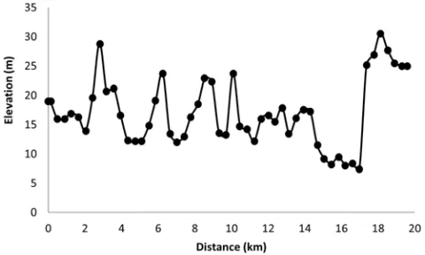
Elevation data for a LOS link between Eket and Akwa Ibom state University are used along with mathematical expressions stated in this paper to determine the various parameters associated with single knife edge diffraction loss. The three values of effective earth radius factors (k-factors) are considered in this paper, namely; k =0.5, k = 0.9 and k = 1.333. The elevation data is given in table 1 and figure 1.

Figure 1. Elevation Profile: Elevation (m) versus Distance.

Table 1. Elevation Profile: Elevation (m) versus Distance.

Distance (m)

Elevation (m)

0.00 19.09 6.63 13.48 13.53 16.23

0.11 19.00 7.01 12.11 13.91 17.66

0.50 16.00 7.40 13.05 14.30 17.36

0.88 16.08 7.78 16.42 14.68 11.52

1.26 16.95 8.16 18.56 15.06 9.29

1.65 16.32 8.55 22.95 15.45 8.34

2.03 14.00 8.93 22.37 15.83 9.50

2.41 19.75 9.31 13.64 16.21 8.14

2.80 28.94 9.70 13.27 16.60 8.37

3.18 20.73 10.08 23.80 16.98 7.49

3.56 21.32 10.46 14.82 17.36 25.17

3.95 16.64 10.85 14.21 17.75 26.92

4.33 12.31 11.23 12.19 18.13 30.65

(4)

5.10 12.27 12.00 16.71 18.90 25.60

5.48 14.86 12.38 15.62 19.28 25.12

5.86 19.24 12.76 17.99 19.59 25.07

6.25 23.77 13.15 13.49

(Data source: Geocontext online topographic profile tool available at: http://www.geocontext.org/publ/2010/04/profiler/en/).

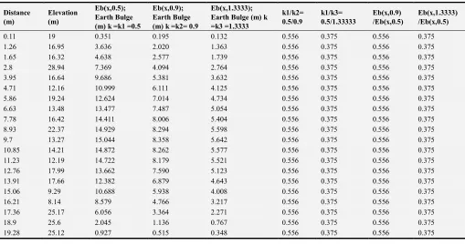
For the three effective earth radius factors (k-factors) considered, namely, k1= 0.5; k2 = 0.9 and k3 = 1.3333, the ratios among the k-factors when compared to the ratio of the earth bulge computed with k-factors are given in Table 2. The results in Table 2 show that according to equation 5

#_{$( ,&')} #_{$( ,&()}=

#$( ,Y.Z)

#$( ,Y.[)= (

'=

.

.\ (21)

Hence;

( , .\)= ( , . )) ._.\* (22)

#_{$( ,&])} #_{$( ,&()}=

#$( ,(.]]]]])

#$( ,Y.[) = (

]=

.

.DDDDD (23)

Hence;

( , .DDDDD)= ( , . )) _.DDDDD. * (24)

In essence, (

' is the k-factor scaling that can be used in

equation (6) to determine the earth bulge at k-factor of when the earth bulge at k-factor of are known.

Table 2. The Effective Earth Radius Adjustment Factor For Earth Bulge Eb(x,k) at distance x where k = k1 = 0.5, k = k2 = 0.9 and k = k3 = 1.3333.

Eb(x,0.5); Earth Bulge (m) k =k1 =0.5

Eb(x,0.9); Earth Bulge (m) k =k2= 0.9

Eb(x,1.3333); Earth Bulge (m) k =k3 =1.3333

k1/k2= 0.5/0.9

k1/k3= 0.5/1.33333

Eb(x,0.9) /Eb(x,0.5)

Eb(x,1.3333) /Eb(x,0.5)

0.11 19 0.351 0.195 0.132 0.556 0.375 0.556 0.375

1.26 16.95 3.636 2.020 1.363 0.556 0.375 0.556 0.375

1.65 16.32 4.638 2.577 1.739 0.556 0.375 0.556 0.375

2.8 28.94 7.369 4.094 2.764 0.556 0.375 0.556 0.375

3.95 16.64 9.686 5.381 3.632 0.556 0.375 0.556 0.375

4.71 12.16 10.999 6.111 4.125 0.556 0.375 0.556 0.375

5.86 19.24 12.624 7.014 4.734 0.556 0.375 0.556 0.375

6.63 13.48 13.477 7.487 5.054 0.556 0.375 0.556 0.375

7.78 16.42 14.411 8.006 5.404 0.556 0.375 0.556 0.375

8.93 22.37 14.929 8.294 5.598 0.556 0.375 0.556 0.375

9.7 13.27 15.044 8.358 5.642 0.556 0.375 0.556 0.375

10.85 14.21 14.872 8.262 5.577 0.556 0.375 0.556 0.375

11.23 12.19 14.722 8.179 5.521 0.556 0.375 0.556 0.375

12.76 17.99 13.662 7.590 5.123 0.556 0.375 0.556 0.375

13.91 17.66 12.382 6.879 4.643 0.556 0.375 0.556 0.375

15.06 9.29 10.688 5.938 4.008 0.556 0.375 0.556 0.375

16.21 8.14 8.579 4.766 3.217 0.556 0.375 0.556 0.375

17.36 25.17 6.056 3.364 2.271 0.556 0.375 0.556 0.375

18.9 25.6 2.045 1.136 0.767 0.556 0.375 0.556 0.375

19.28 25.12 0.927 0.515 0.348 0.556 0.375 0.556 0.375

Again, for the three effective earth radius factors (k-factors) considered, (k1= 0.5; k2 = 0.9 and k3 = 1.3333), the adjustment factors for diffraction parameter, V(x,k) at distance x are given in table 3. The results in Table 3 show that according to equation 16 for k1 =0.5 and k2= 0.9

9( , .\)= 9( , )+ ^ ( , . )) ._.\− 1*_ HJ_ʎ ( )_{( )} < _{( )}( )I (25)

Also, according to equation 19 for k1 =0.5 and k2= 0.9,

9( , .\)= 9( , . )+ 9K( . , .\)

Also, results in Table 3 show that for k1 =0.5 and k3= 1.33333

9( , .DDDDD)= 9( , )+ ^ ( , . )) ._.\− 1*_ HJ_ʎ ( )_{( )} < _{( )}( )I (26)

9( , .DDDDD)= 9( , . )+ 9K( . , .DDDDD) (27)

In essence, H _{( ,7 )}) (

'− 1*I :;

( ) < ( )

ʎ ( ) ( ) > is the

(5)

Table 3. The Effective Earth Radius Adjustment Factor For Diffraction Parameter, V(x,k) at distance x where k = k1 = 0.5, k = k2 = 0.9 and k = k3 = 1.3333.

X = Distance (m)

V(x,k1) = V(x,0.5)

V(x,k2) = V(x,0.9) =

V(x,k3) = V(x,1.3333)

Vc(k1,k2)= Adjustment Factor For k1 and k2

Vc(k1,k3) = Adjustment Factor For k1 and k3

V(x,k2) = V(x,k1) + Vc(k1,k2)

V(x,k3) = V(x,k1) +Vc(k1,k3)

0.5 16 -24.424 -25.602 -26.081 -1.178 -1.657 -25.602 -26.081

1.65 16.32 -5.711 -6.818 -7.268 -1.107 -1.557 -6.818 -7.268

2.8 28.94 1.381 0.345 -0.076 -1.036 -1.457 0.345 -0.076

3.95 16.64 -1.338 -2.303 -2.695 -0.965 -1.357 -2.303 -2.695

4.71 12.16 -1.759 -2.677 -3.05 -0.918 -1.291 -2.677 -3.05

5.86 19.24 -0.153 -1 -1.344 -0.847 -1.191 -1 -1.344

6.63 13.48 -0.822 -1.621 -1.946 -0.8 -1.124 -1.621 -1.946

7.78 16.42 -0.3 -1.028 -1.324 -0.729 -1.025 -1.028 -1.324

8.93 22.37 0.345 -0.312 -0.58 -0.658 -0.925 -0.312 -0.58

9.7 13.27 -0.524 -1.134 -1.382 -0.61 -0.858 -1.134 -1.382

10.85 14.21 -0.434 -0.973 -1.192 -0.539 -0.758 -0.973 -1.192

11.23 12.19 -0.599 -1.115 -1.325 -0.516 -0.725 -1.115 -1.325

12 16.71 -0.277 -0.746 -0.936 -0.468 -0.659 -0.746 -0.936

13.15 13.49 -0.561 -0.958 -1.12 -0.397 -0.559 -0.958 -1.12

14.3 17.36 -0.386 -0.712 -0.845 -0.326 -0.459 -0.712 -0.845

15.83 9.5 -0.956 -1.188 -1.282 -0.232 -0.326 -1.188 -1.282

16.98 7.49 -1.138 -1.299 -1.365 -0.161 -0.226 -1.299 -1.365

17.75 26.92 -0.223 -0.336 -0.382 -0.114 -0.16 -0.336 -0.382

18.9 25.6 -0.432 -0.474 -0.491 -0.043 -0.06 -0.474 -0.491

19.28 25.12 -0.502 -0.521 -0.528 -0.019 -0.027 -0.521 -0.528

Once more, for the three effective earth radius factors (k-factors) considered, (k1= 0.5; k2 = 0.9 and k3 = 1.3333), the adjustment factors for O_{PQ( ,7)} (the Fresnel zone in which the tip of a single knife edge obstruction lies) are given in table 4. The results in Table 4 show that for k1 =0.5 and k2= 0.9

OPQ( , .\)= OPQ( , . )+ O PQK( . , .\) (28)

where

OPQK( . , .\)= S( ,Y[) ST(Y.[,Y.Z)< ST(Y.[,Y.Z)

'

(29)

Also, results in Table 4 show that for k1 =0.5 and k3= 1.33333

OPQ( , .DDDDD)= OPQ( , . )+ OPQK( . , .DDDDD) (30)

where

OPQK( . , .DDDDD)= S( ,Y[) ST(Y.[,(.]]]]])< ST(Y.[,(.]]]]])

'

(31)

In essence, H S( ,&() ST(&(,&')< ST(&(,&')

'

I is the k-factor adjustment factor that can be used in equation (24) to determine the O_{PQ( ,7)} at distance x and k-factor of when the O_{PQ( ,7)}at distance x and k-factor of are known.

Table 4. Effective earth radius adjustment factors for O_{PQ( ,7)} (the Fresnel zone in which the tip of a single knife edge obstruction lies).

Distance (m) `_abc(d,e_f₎ `_abc(d,e_g₎ `_abc(d,e_h₎ `_abci(e_f_,e_g₎ `_abci(e_f_,e_h₎ `_`abc(d,eg) = `abc(d,ef)+

abci(ef,eg)

`abc(d,eh)= `abc(d,ef)+

`abci(ef,eh)

1.65 16.31 23.24 26.41 6.94 10.10 23.24 26.41

2.8 0.95 0.06 0.00 -0.89 -0.95 0.06 0.00

3.95 0.90 2.65 3.63 1.76 2.74 2.65 3.63

4.71 1.55 3.58 4.65 2.04 3.10 3.58 4.65

5.86 0.01 0.50 0.90 0.49 0.89 0.50 0.90

6.63 0.34 1.31 1.89 0.98 1.56 1.31 1.89

7.78 0.04 0.53 0.88 0.48 0.83 0.53 0.88

8.93 0.06 0.05 0.17 -0.01 0.11 0.05 0.17

9.7 0.14 0.64 0.95 0.51 0.82 0.64 0.95

10.08 0.08 0.02 0.09 -0.07 0.00 0.02 0.09

11.23 0.18 0.62 0.88 0.44 0.70 0.62 0.88

12.76 0.03 0.21 0.34 0.19 0.31 0.21 0.34

13.91 0.06 0.24 0.34 0.18 0.29 0.24 0.34

14.68 0.30 0.57 0.71 0.28 0.42 0.57 0.71

15.83 0.46 0.71 0.82 0.25 0.36 0.71 0.82

16.98 0.65 0.84 0.93 0.20 0.28 0.84 0.93

17.75 0.02 0.06 0.07 0.03 0.05 0.06 0.07

18.51 0.04 0.06 0.07 0.02 0.03 0.06 0.07

(6)

4. Conclusion

The influence of effective earth radius k-factor on various parameters associated with single knife edge diffraction are studied. Specifically, analytical expressions for the k-adjustment factors that can be used to determine the various parameters associated with single knife edge diffraction are derived. With the k-adjustment factors, the value of the given parameter can be determined at any other k-factor if the parameter value is known at any one k-factor.

The k-adjustment factors are validated using empirical elevation profile data for line-of-sight (LOS) communication link between Eket and Akwa Ibom state University. The k-adjustment factors considered are for the following three parameters, the earth bulge, Fresnel-Kirchoff diffraction parameter and the number of Fresnel zones that are partially or fully blocked by obstruction in the signal path. In all, the results show that when the value of any of the three parameters is known at a given k-factor, k1, then the value of that parameter can be determined at any other k-factor, say k2 by adding the k-adjustment factor of that parameter to the value of the parameter at k1.

References

[1] Göktas, P. (2015). Analysis and implementation of prediction models for the design of fixed terrestrial point-to-point systems (Doctoral dissertation, bilkent university).

[2] Al Mahmud, M. R. (2009). Analysis and planning microwave link to established efficient wireless communications (Doctoral dissertation, Blekinge Institute of Technology).

[3] Bogucki, J., & Wielowieyska, E. (2013). Fading duration in line-of-sight radio links at 6 GHz. Journal of Telecommunications and Information Technology, (2), 14-18. [4] Göktaş, P., Altvntaş, A., Topçu, S., & Karaşan, E. (2014,

August). The effect of terrain roughness in the microwave line-of-sight multipath fading estimation based on Rec. ITU-R P. 530-15. In General Assembly and Scientific Symposium (URSI GASS), 2014 XXXIth URSI (pp. 1-4). IEEE.

[5] Smith, B., & Carpentier, M. H. (2012). The microwave engineering handbook: Microwave systems and applications (Vol. 3). Springer Science & Business Media.

[6] Thakur, A., Kamboj, S., & Scholar, P. G. (2016). Transmission and Optimization of a 3G Microwave Network at 18 GHz. International Journal of Engineering Science, 5622.

[7] Fussen, D., Tétard, C., Dekemper, E., Pieroux, D., Mateshvili, N., Vanhellemont, F.,... & Demoulin, P. (2015). Retrieval of

vertical profiles of atmospheric refraction angles by inversion of optical dilution measurements. Atmospheric Measurement Techniques, 8 (8), 3135-3145.

[8] Waheed-uz-Zaman, M., & Jan, M. (2013). To Study the Implications of the Evaporation Duct for Ground Waves Path in Pakistan Coastal Water through Statistical Assessment. Journal of American Science, 9 (6).

[9] Mufti, N. (2012). Investigation into the Effects of the Troposphere on Vhf and Uhf Radio Propagation and Interference between Co-Frequency Fixed Links (Doctoral dissertation, University of Leicester).

[10] Seybold, J. S. (2005). Introduction to RF propagation. John Wiley & Sons.

[11] Mangum, J. G., & Wallace, P. (2015). Atmospheric Refractive Electromagnetic Wave Bending and Propagation Delay. Publications of the Astronomical Society of the Pacific, 127 (947), 74.

[12] Vollmer, M. (2003). A simple method for estimating the thickness of the atmosphere by light scattering. American Journal of Physics, 71 (10), 979-983.

[13] Serdega, V., & Ivanovs, G. (2015). Refraction seasonal variation and that influence on to GHz range microwaves availability. Elektronika ir Elektrotechnika, 78 (6), 39-42. [14] Adediji, A. T., Mandeep, J. S., & Ismail, M. (2014).

Meteorological Characterization of Effective Earth Radius Factor (k-Factor) for Wireless Radio Link Over Akure, Nigeria. Mapan, 29 (2), 131-141.

[15] Doerry, A. W. (2013). Earth Curvature and Atmospheric Refraction Effects on Radar Signal Propagation. Sandia Report SAND2012-10690.

[16] Abu-Almal, A., & Al-Ansari, K. (2010). Calculation of effective earth radius and point refractivity gradient in UAE. International Journal of Antennas and Propagation, 2010. [17] Nyete, A. M., & Afullo, T. J. O. (2013). Seasonal distribution

modeling and mapping of the effective earth radius factor for microwave link design in South Africa. Progress In Electromagnetics Research B, 51, 1-32.

[18] Freeman, R. L. (2006). Radio system design for telecommunication (Vol. 98). John Wiley & Sons.

[19] Wright, E., & Reynders, D. (2004). Practical telecommunications and wireless communications: for business and industry. Elsevier.