Estimating Functions for Blind Separation When Sources Have
Variance Dependencies
Motoaki Kawanabe [email protected]
Fraunhofer FIRST.IDA Kekul´estrasee 7 12489 Berlin, Germany
Klaus-Robert M ¨uller [email protected]
Fraunhofer FIRST.IDA Kekul´estrasse 7
12489 Berlin, Germany and Department of Computer Science University of Potsdam
August-Bebel-Strasse 89 14482 Potsdam, Germany
Editor: Aapo Hyv¨arinen
Abstract
A blind separation problem where the sources are not independent, but have variance dependencies is discussed. For this scenario Hyv¨arinen and Hurri (2004) proposed an algorithm which requires no assumption on distributions of sources and no parametric model of dependencies between com-ponents. In this paper, we extend the semiparametric approach of Amari and Cardoso (1997) to variance dependencies and study estimating functions for blind separation of such dependent sources. In particular, we show that many ICA algorithms are applicable to the variance-dependent model as well under mild conditions, although they should in principle not. Our results indicate that separation can be done based only on normalized sources which are adjusted to have station-ary variances and is not affected by the dependent activity levels. We also study the asymptotic distribution of the quasi maximum likelihood method and the stability of the natural gradient learn-ing in detail. Simulation results of artificial and realistic examples match well with our theoretical findings.
Keywords: blind source separation, variance dependencies, independent component analysis,
semiparametric statistical models, estimating functions
1. Introduction
s(t) = (s1(t), . . . ,sn(t) )>, and the observed signals by x(t) = (x1(t), . . . ,xm(t) )>. In this paper,1 we will focus on real-valued signals. The mixing can be expressed as the equation
x(t) =As(t),
where A= (ai j)denotes the mixing matrix. For simplicity, we consider the case where the number of source signals equals that of observed signals (n=m). Both the sources s(t) and the mixing matrix A are unknown, and the goal is to estimate them based on the observation x(t)alone.
In most blind source separation (BSS) methods, the source signals are assumed to be statisti-cally independent. Blind source separation based on such a model is called independent component analysis (ICA). By using non-Gaussianity of the sources, the mixing matrix can be estimated and the source signals can be extracted under appropriate conditions. There are also further approaches of BSS, that are, for example, based on second-order statistics and algorithms exploiting nonstation-arity. The second-order methods are applicable to the case where the source signals have (lagged) auto-correlation. Provided that components have nonstationary, smoothly changing variances, the model can be estimated as well by algorithms based on nonstationarity of signals.
Among many extensions of the basic ICA models, several researchers have studied the case where the source signals are not independent (for example, Cardoso, 1998b; Hyv¨arinen et al., 2001a; Bach and Jordan, 2002; Valpola et al., 2003, see also references in Hyv¨arinen and Hurri, 2004). The dependencies either need to be exactly known beforehand, or they are simultaneously estimated by the algorithms. Recently, a novel idea called double-blind approach was introduced by Hyv¨arinen and Hurri (2004). In contrast to previous work, their method requires no assumption on the distri-butions of the sources and no parametric model of the dependencies between the components. They simply assume that the sources are dependent only through their variances and that the sources have temporal correlation. In the Topographic ICA (Hyv¨arinen et al., 2001a), the dependencies of the sources are also caused only by their variances, but in contrast to the double blind case, they are determined by a prefixed neighborhood relation. It should be noted that for such dependent compo-nent models identifiability results have not been theoretically established so far, while identifiability of multidimensional ICA was proven by Theis (2004).
A statistical basis of ICA was established by Amari and Cardoso (1997). They pointed out that the ICA model is an example of semiparametric statistical models (Bickel et al., 1993; Amari and Kawanabe, 1997a,b) and studied estimating functions for it. In particular, they showed that the quasi maximum likelihood (QML) estimation and the natural gradient learning give a correct solution re-gardless of the true source densities which satisfy certain mild conditions. In this paper, we extend their approach to the BSS problem considered in Hyv¨arinen and Hurri (2004). Investigating esti-mating functions for the model, we show that many of ICA algorithms based on the independence assumption can achieve consistent solutions in a local sense, even if there exist variance depen-dencies, which is astonishing and seems somewhat counterintuitive. We remark that estimating functions are concerned with local consistency (’consistency’ will denote its local version in the following) and in general have spurious solutions. For a few algorithms, even global consistency has been proven by different principles (for example, Hyv¨arinen and Hurri, 2004). Nevertheless, our result goes beyond existing ones, because it covers most types of BSS algorithms and can give asymptotic distributions. The main message of this paper is that most ICA algorithms can be proven to be consistent in our framework although the data is not independent. So they must effectively
use some concept beyond independence. Thus our consistency results indicate that separation can be done based only on normalized sources which are adjusted to have stationary variances and is not affected by the dependent activity levels.
This paper is organized as follows. At first, we define the variance-dependent model in Section 2 and explain estimating functions, a useful tool for discussing semiparametric estimators in Section 3. In Section 4, we discuss the relation between estimating functions for the ICA model and those for the variance-dependent BSS model in general. It is shown that these algorithms work properly, even if there exist spatiotemporal variance dependencies. Among several ICA algorithms, the quasi maximum likelihood method and its online version, the natural gradient learning are discussed in detail. We study the asymptotic distributions of the quasi maximum likelihood method (Section 5.1) and the stability of the natural gradient learning (Section 5.2). We also give a brief summary about several other ICA algorithms from our viewpoint in Section 5.3. Detailed discussion can be found in Appendix A. The theoretical insights are underlined by several numerical simulations in Section 6. In particular, we carried out two experiments, where we extract two speech signals with high variance dependencies. It is sometimes believed that ICA algorithms work for mixture of acoustic signals or natural images because the data are sparse and often disjoint. Our results show that they can also separate even highly coherent signals, and our theoretical analysis can thus help to understand the reason.
2. Variance-Dependent BSS Model
Hyv¨arinen and Hurri (2004) formalized the probabilistic framework of variance-dependent blind separation. Let us assume that each source signal si(t) is a product of non-negative activity level vi(t)and underlying i.i.d. signal zi(t), that is,
si(t) =vi(t)zi(t). (1)
We remark that the sequences of the vectors s= (s1, . . . ,sn)>, v= (v1, . . . ,vn)>and z= (z1, . . . ,zn)> are considered as multivariate random processes in this paper. In practice, the activity levels vi(t) are often dependent among different signals and each observed signal is expressed as
xi(t) = n
∑
j=1ai jvj(t)zj(t), i=1, . . . ,n,
where vi(t)and zi(t)satisfy:
(i) vi(t)and zj(t0)are independent for all i, j, t and t0,
(ii) each zi(t)is i.i.d. in time for all i, the random vector z= (z1, . . . ,zn)>is mutually independent,
(iii) zi(t)have zero mean and unit variance for all i.
=
=
×
×
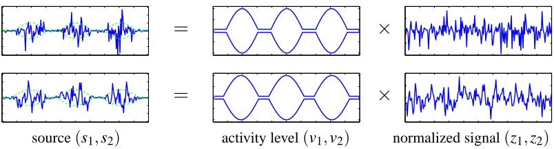
source(s1,s2) activity level(v1,v2) normalized signal(z1,z2)
Figure 1: Sources(s1,s2)with variance dependencies in the variance-dependent BSS model. In the middle panels both viand−vi are plotted for clarity.
However, since the sequences z1and z2are multiplied by extremely dependent activity levels v1and v2, respectively, the short-term variance of the source signals s1and s2are highly correlated.
Hyv¨arinen and Hurri (2004) proposed an algorithm which maximizes the objective function
J(W) =
∑
i,j
[covc([w>i u(t)]2,[w>j u(t−∆t)]2) ]2,
wherecov denotes the sample covariance, Wc = (w1, . . . ,wn)> is constrained to be orthogonal and where u(t) is obtained by preprocessing the signal x(t) by spatial whitening. It was proved that the objective function J is maximized when WA equals a signed permutation matrix, if the matrix K= (Ki j) = (cov{s2i(t),s2j(t−∆t)})is of full rank. This method shows good performance as long as there exist temporal variance dependencies and the data is not spoiled by outliers (see Meinecke et al., 2004).
It is important to remark that the nonstationary algorithm by Pham and Cardoso (2000) was also designed for the same source model (1), except that vi(t)’s are assumed to be deterministic and slowly varying. However, it is straightforward to show validity of this algorithm, when vi(t)’s are (slowly-varying) random sequences.
3. Semiparametric Statistical Models and Estimating Functions
Amari and Cardoso (1997) established a statistical basis of the ICA problem. They pointed out that the standard ICA model2
p(X|B,ρs) =|det B|T T
∏
t=1n
∏
i=1ρsi{b
>
i x(t)} (2)
is an example of semiparametric statistical models (Bickel et al., 1993; Amari and Kawanabe, 1997a,b), where B= (b1, . . . ,bn)> =A−1 is the demixing matrix to be estimated and ρs(s) =
n
Π
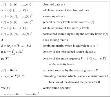
i=1ρsi(si) is the density of the sources s. Notations used in the following sections are also sum-marized in Table 1. As the function ρs in this model, semiparametric statistical models contain infinite dimensional or functional nuisance parameters which are difficult to estimate. Moreover, they even disturb inference on parameters of interest.
x(t) = (x1(t), . . . ,xn(t) )> observed data at t
X= (x(1), . . . ,x(T) ) whole sequence of the observed data
s(t) = (s1(t), . . . ,xn(t) )> source signals at t
v(t) = (v1(t), . . . ,vn(t) )> general activity levels of the sources s(t)
V = (v(1), . . . ,v(T) ) whole sequence of the activity levels
z(t) = (z1(t), . . . ,zn(t) )> normalized source signals by the activity levels v(t)
A n×n mixing matrix
B= (bi j) = (b1, . . . ,bn)> demixing matrix which is equivalent to A−1
ρz(z) = n
Π
i=1ρzi(zi) density of the normalized source signals z
ρV(V) density of the entire sequence V= (v(1), . . . ,v(T) )
of the activity levels
y(t) =Bx(t) extracted sources by the demixing matrix B
F(x,B)or ¯F(X,B) estimating function which is an n×n matrix-valued
function of the data and the parameter B
vec(F) vectorization operator
= (F11, . . . ,Fn1, . . . ,F1n, . . . ,Fnn)>
Table 1: List of notations used in the variance-dependent BSS model
In the variance-dependent BSS model which we consider, the sources s(t) are decomposed of two components, the normalized signals z(t) = (z1(t), . . . ,zn(t) )> and the general activity levels v(t) = (v1(t), . . . ,vn(t) )>. Since the former has mutual independence like the ICA model, the den-sity of the data X is factorized as
p(X|V ; B,ρz) =|det B|T T
∏
t=1n
∏
i=11 vi(t) ρzi
(
b>i x(t) vi(t)
)
, (3)
when V= (v(1), . . . ,v(T) )is fixed. Therefore, the marginal distribution can be expressed as
p(X|B,ρz,ρV) =
Z
p(X|V ; B,ρz)ρV(V)dV, (4)
where the densityρV of V becomes an extra nuisance function.
In order to construct valid estimators for such semiparametric models, estimating functions were introduced by Godambe (1976). Let us consider a general semiparametric model p(x|θ,ρ), where
for anyθandρ(Godambe, 1991),
E[f(x,θ)|θ,ρ] =0,
|det Q| 6=0, where Q=E
∂
∂θf(x,θ)
θ,ρ
,
Ekf(x,θ)k2θ,ρ<∞,
where E[·|θ,ρ]denotes the expectation over x with the density p(x|θ,ρ)andk · kis the Euclidean norm. Suppose i.i.d. samples x(1), . . . ,x(T) are obtained from the model p(x|θ∗,ρ∗). If such a function exists, by solving the estimating equation
T
∑
t=1f(x(t),bθ) =0, (5)
we can get an estimatorbθwith good asymptotic property. Such an estimator that is a solution of an estimating equation as (5) is called an M-estimator in statistics (Huber, 1981). It can be regarded as an extension of the maximum likelihood method for parametric models. The M-estimatorbθis consistent regardless of the true nuisance parameter ρ∗, when the sample size T goes to infinity. Moreover, it is asymptotically Gaussian distributed, that is,bθ∼N(θ∗,Av), where Av denotes the asymptotic variance computed by the following equation
Av=Av(θ∗,ρ∗) = 1
T Q
−1Eh f(x,θ)f>(x,θ)
θ∗,ρ∗i(Q−1)>,
and Q=Q(θ∗,ρ∗) =Eh ∂
∂θf(x,θ)
θ∗,ρ∗i. We remark that the asymptotic variance Av depends on the true parameters(θ∗,ρ∗), but not on the data x(1), . . . ,x(T). As we will explain in Section 4.2, notions of estimating functions and M-estimators were extended to non i.i.d cases.
Although estimating functions are useful for semiparametric models, it is non-trivial to find such functions. Amari and Kawanabe (1997a,b) studied this problem from a geometrical point of view and gave a guideline for discussing estimating functions.
The asymptotic result guarantees theoretically that the estimatorbθderived from the estimating function converges to the true parameterθ∗ under mild conditions. However, we should remark that the asymptotic variance Av of the estimator depends on the true nuisance parameterρ∗. For example, when the matrix Q is almost singular at ρ∗, it can happen that the asymptotic variance Av becomes very large. This may cause some practical problem, that is, the estimate from finite samples can be no longer close to the true parameter. We will revisit this issue in Section 6.
Furthermore, online algorithms with similar consistency property can also be constructed from estimating functions,
θt+1 = θt−ηt f(x(t),θt), (6)
4. General Properties of Estimating Functions for Blind Separation
In this section we will at first review estimating functions for the ICA model (2) (see also Amari and Cardoso, 1997; Cardoso, 1997) and then discuss our contribution, that is, by defining estimating functions for the variance-dependent BSS model (3) and (4).
4.1 Estimating Functions for Ordinary Blind Source Separation
In case of the ICA model, the parameter of interest is the n×n matrix B=A−1and hence it is con-venient to write the estimating functions in n×n matrix form F(x,B). The conditions of estimating functions are reshaped accordingly as
E[F(x,B)|B,ρs] =0, (8)
|det Q| 6=0, where Q=E
∂
vec{F(x,B)}
∂vec(B)
B,ρs
, (9)
EkF(x,B)k2 F
B,ρs
<∞, (10)
where vec(F) = (F11, . . . ,Fn1, . . . ,F1n, . . . ,Fnn)> is the vectorization of matrices andk · kF denotes Frobenius norm. It should be noted that both in usual ICA models and in the variance-dependent BSS model, scales and orders of the sources cannot be determined, that is, two matrices B and PDB indicate the same distribution, when P and D are a permutation and a diagonal matrix respectively (Comon, 1994).3 Therefore, we can find any matrix in the equivalence class, so for notational convenience we will fix scales as the constraints (25) later.4
One of the standard ICA algorithms originates from maximum likelihood estimation, which is asymptotically the best method if the densityρsis known. Because in the semiparametric modelρs is unknown and difficult to estimate, the idea is to use instead the maximum likelihood estimation under a prefixed densityeρs. The method is called the quasi maximum likelihood estimation, since the fixedeρsdoes not coincide with the true one. The estimatorB is derived from the equationb
T
∑
t=1h
I−ϕ{y(t)}y>(t)i=0, (11)
where y(t) =Bxb (t)is the estimator of the sources,ϕ(y) = (ϕ1(y1), . . . ,ϕn(yn) )> and
ϕi(yi) =− d
dyilogeρsi(yi).
For the nonlinear functionϕi(yi),
ϕi(yi) = tanh(c yi), c>0, (12)
ϕi(yi) = y3i, (13)
are often employed. The function F(x,B) =I−ϕ{Bx}(Bx)> in (11) is an example of estimating functions for the ICA model, provided that it satisfies (9) and (10). It is trivial to show that it fulfills (8). Another example is the function
F(x,B) =Bx(Bx)>−I+ (Bx)g>(Bx)−g(Bx) (Bx)>
3. It is clear that the variance-dependent BSS model has at least such indeterminacy. On the other hand, the identifiability in this case has not been proved so far.
for FastICA (see (37) in Appendix A.1), where g(·)is a vector valued non-linear function asϕ(·). We remark that this procedure can also be derived from minimum mutual information (Yang and Amari, 1997) and infomax principle (Bell and Sejnowski, 1995).
In general the quasi maximum likelihood estimator is no longer consistent because of misspec-ified distribution. However, in the ICA model (2), Amari and Cardoso (1997) found that the quasi maximum likelihood method and its online version (the natural gradient learning) give an asymp-totically consistent estimator, provided that F(x,B) =I−ϕ{Bx}(Bx)> satisfies (9) and (10). In particular, we remark that the assumed distributioneρsis not equal to the true one. This research has motivated us to investigate also such semiparametric procedures for the variance-dependent BSS model (3) and (4). In particular, we will show in Section 5.1 that the quasi maximum likelihood method (11) still gives a consistent estimator even under this extended situation.
4.2 Estimating Functions for Variance-Dependent Blind Source Separation
In the variance-dependent BSS model, in contrast to the ICA model studied by Amari and Cardoso (1997), the data sequence X = (x(1), . . . ,x(T) )is not i.i.d. in time, but might have time depen-dencies. Therefore, we have to consider more general functions ¯F(X,B)of the whole sequence X . General estimating functions ¯F(X,B)must satisfy
E[F¯(X,B)|B,ρz,ρV] =0, (14)
|det Q| 6=0, where Q=E
∂
vec{F¯(X,B)}
∂vec(B)
B,ρz,ρV
, (15)
EkF¯(X,B)k2 F
B,ρz,ρV
<∞, (16)
for all(B,ρz,ρV). An M-estimatorB can be derived from the estimating equationb
¯
F(X,Bb) =0. (17)
Suppose that the data X is subject to p(X|B∗,ρ∗z,ρ∗V)defined by (3) and (4).
Theorem 1 If the function ¯F(X,B)satisfies the conditions (14) – (16) and appropriate regularity
conditions such as Condition 2.6 in Sørensen (1999), the M-estimatorB derived from the equationb
(17) is asymptotically Gaussian distributed vec(Bb)∼N(vec(B∗),Av), where
Av = Av(B∗,ρ∗z,ρ∗V) = Q−1Σ(Q−1)>, (18)
Σ = Σ(B∗,ρ∗z,ρ∗V) = E
h
vec{F¯(X,B∗)}vec{F¯(X,B∗)}>B∗,ρ∗ z,ρV∗
i
Q = Q(B∗,ρ∗z,ρV∗) = E
∂
vec{F¯(X,B∗)}
∂vec(B)
B∗,ρ∗z,ρV∗
.
Proof See Sørensen (1999).
Now, we investigate the relation between estimating functions for the ICA model and those for the variance-dependent BSS model. Let F(x,B) be an estimating function for the ICA model. In the ICA context it is often the case that such estimating functions satisfy
for any diagonal matrix D, that is, its off-diagonal parts (19) hold for all matrices equivalent to B. The scale factor D is determined usually by the diagonal parts of condition (8)
E[Fii(x,B)|B,ρs] =0,
in the ordinary ICA model. We will soon present the equation for fixing the scale factor D in the variance-dependent BSS model.
Let us consider the function
¯
F(X,B) = T
∑
t=1F(x(t),B), (20)
which is used in estimating equations for the ICA model.5 We can show that this function becomes a candidate of estimating functions for the variance-dependent BSS model.
Proposition 2 The function ¯F(X,B)defined in (20) satisfies condition (14), provided that F(x,B)is an estimating function for the ICA model and fulfills (19). Furthermore, if the additional assumption
EkF(x(t),B)k2F B,ρz,ρV
<∞, ∀t (21)
holds, condition (16) is also satisfied.
Proof Taking expectations of the off-diagonal terms of (14), we get
EF¯i j(X,DB)
B,ρz,ρV
= E
"
T
∑
t=1EFi j(x(t),DB)
V ; B,ρz
ρV
#
= E
"
T
∑
t=1EFi j(x(t),DB)
B,ρs|v(t) ρV
#
whereρs|v(t)is the density function of s(t)when its activity level is fixed at v(t), that is,
ρs|v(t)(s) =
n
∏
i=11 vi(t)
ρzi
si vi(t)
.
We remark that the expectation E[·|V ; B,ρz]( E[·|B,ρs|v(t)]) is taken over z(t)(resp. s(t)) under fixed
activity levels V , while E[·|ρV]denotes the expectation over the activity level V . Because (19) holds for anyρs, we can prove
EF¯i j(X,DB)
B,ρz,ρV
=0,
for all diagonal matrices D. If we select the scale factor D such that the diagonal terms
E[F¯ii(X,B)|B,ρz,ρV] =0
hold, ¯F satisfies the unbiasedness condition (14). We furthermore note that this scaling is different from that in the ICA model presented before, and the expectation EFii(x(t),B)|B,ρs|v(t)
at each time t can be non-zero in general.
The left hand side of Eq. (16) can be expressed as
EkF¯(X,B)k2 F
B,ρz,ρV
= E
"
∑
t,t0E
h
tr{F(x(t),B)F>(x(t0),B)}V ; B,ρz
i ρV # = E
∑
tEkF(x(t),B)k2 F
B,ρs|v(t) ρV +E "
∑
t6=t0n
∑
i=1EFii(x(t),B)|B,ρs|v(t)EFii(x(t0),B)B,ρs|v(t0) ρV # , (22)
where we used the fact that x(t)and x(t0) (t6=t0) are independent for fixed V . From assumption (21), the first term of Eq. (22) is finite.
∑
tEEkF(x(t),B)k2F B,ρs|v(t) ρV
=
∑
t
EkF(x(t),B)k2 F
B,ρz,ρV
<∞ (23)
We remark that condition (10) does not necessarily imply assumption (21). Let us define c(v(t) ):=EkF(x(t),B)k2
F
B,ρs|v(t)
. Since
EFii(x(t),B)|B,ρs|v(t)≤ q
EFii2(x(t),B)B,ρs|v(t)
≤pc(v(t) ),
the second term of Eq. (22) (called r in the following) can be bounded as
|r| < n
∑
t6=t0Eh pc(v(t) )pc(v(t0) )ρ V i ≤ n
∑
t pE[c(v(t) )|ρV]
2
≤ nT
∑
tE[c(v(t) )|ρV].
Here we used Schwarz’s inequality twice. Because of Eq. (23), this bound is also finite.
The basic idea of this proof is that the situation becomes similar to the ordinary ICA model, if the activity levels V are fixed. Unfortunately, the other conditions are difficult to be proven in this general form. For example, the second condition can be transformed in the similar way as
E
∂
vec{F¯(X,B)}
∂vec(B)
B,ρz,ρV
= T
∑
t=1E
E
∂
vec{F(x(t),B)}
∂vec(B)
B,ρs|v(t) ρV
. (24)
Even if each term E
h∂
vec{F(x(t),B)}
∂vec(B)
B,ρs|v(t) i
5. Consistency Results for Variance Dependent Blind Source Separation Using the Estimating Function Framework
We will use the estimating function framework to prove consistency results for (i) the quasi max-imum likelihood type methods (for example, Pham and Garrat, 1997; Bell and Sejnowski, 1995), (ii) the natural gradient learning for ICA (for example, Amari, 1998) and (iii) various other ICA al-gorithms such as FastICA (Hyv¨arinen and Oja, 1997), TDSEP/SOBI (Ziehe and M¨uller, 1998; Be-louchrani et al., 1997), ’Sepagaus’ (Pham and Cardoso, 2000) and JADE (Cardoso and Souloumiac, 1993).
5.1 Asymptotic Distribution of the Quasi Maximum Likelihood Estimator
In this section, it is shown that the quasi maximum likelihood method (11) as for example Pham and Garrat (1997); Bell and Sejnowski (1995) still gives a consistent estimator even under the extended model (3) and (4). For convenience, we fix the scales of the recovered signals as
E
"
T
∑
t=1ϕi{b>i x(t)}b>i x(t)
B,ρz,ρV #
=T, (25)
for i=1, . . . ,n. Then (14) is automatically fulfilled for the diagonal terms. We remark that by this constraints the length of bi’s may depend on the nuisance parameters (ρz,ρV), but this does not change the following discussion, because the scales can be fixed arbitrarily.
Since the function F(x,B) =I−ϕ{Bx}(Bx)> obviously satisfies (19), we already know from Theorem 2 that the function
¯
FQML(X,B) = T
∑
t=1h
I−ϕ{y(t)}y>(t)i
satisfies the conditions (14) and (16) under the assumption
Eϕ2i{yi(t)}y2j(t)B,ρz,ρV
<∞, ∀i, j, t, (26)
where y(t)denotes the extracted sources Bx(t). The additional assumption imposes mild restriction on the distribution of the activity levels V . For example, when the densityρV has extremely heavy tails, the left hand side of Eq. (16) becomes infinite, even if condition (10) is fulfilled. Thus, we need assumptions like (26) to exclude such unusual cases.
For better understanding, we directly analyze the off-diagonal terms of (14)
E
"
T
∑
t=1ϕi{yi(t)}yj(t)
B,ρz,ρV #
= T
∑
t=1E Eϕi{vi(t)zi(t)} vj(t)zj(t)
V ; B,ρz ρV
= T
∑
t=1E E[ϕi{vi(t)zi(t)} |V ; B,ρz]E
vj(t)zj(t)
V ; B,ρz ρV
= 0.
To prove condition (15) and compute the asymptotic variance (18), we calculate the n2×n2 matrix Q. If we use the non-holonomic basis dχ=dBB−1(Amari et al., 2000), Q is expressed as
Q=E
∂
vec(F¯QML)
∂vec(χ)
B,ρz,ρV
¯ B−1,
where ¯B= (B¯i j;kl) and ¯Bi j;kl =δikbl j. Fortunately, the matrix Eh∂vec(F¯QML)
∂vec(χ)
i
turns out to have a
simple structure such that only the following 2n2−n components are non-zero,
E
"
∂F¯QML ii ∂χii # = − T
∑
t=1E[mi{vi(t)}]−T,
E "
∂F¯QML i j
∂χi j
#
E
"
∂F¯QML i j
∂χji
#
E
"
∂F¯QML ji
∂χi j
#
E
"
∂F¯QML ji ∂χji # = − T Σ
t=1E
[ki{vi(t)}v2j(t) ] T
T ΣT
t=1E[kj{vj(t)}v 2 i(t) ]
,
in which we employed the following quantities
ki{vi(t)} = E[ϕ˙i{vi(t)zi(t)} |V ; B,ρz], mi{vi(t)} = v2i(t)E
˙
ϕi{vi(t)zi(t)}z2i(t)
V ; B,ρz
,
and ˙ϕiis the derivative ofϕi. Hence, it is not difficult to check non-singularity of this matrix, and if this is the case, the condition (15) holds. We can also explicitly calculate the inverse matrix
Q−1=B¯Eh∂vec(F¯QML)
∂vec(χ)
i−1
that appears in the asymptotic variance (18), because we only have to invert the 2×2 matrices.
Finally, the variance of the estimating function can be computed as
E
h
¯
Fi jQMLF¯klQML|B,ρz,ρV
i =
∑
t,t0covϕi{yi(t)}yi(t), ϕk{yk(t0)}yk(t0)
, i= j, k=l
∑
tEϕi{yi(t)}ϕk{yk(t)}y2j(t)
, j=l,i6=j or k6=l
∑
tE[ϕi{yi(t)}yi(t)ϕj{yj(t)}yj(t) ], i=l, j=k, i6= j
which is slightly more complicated than the standard ICA model. Summing up the discussion above, we get the following theorem.
Theorem 3 Suppose that the conditions T
∑
t=1E[mi{vi(t)}] +T 6=0, ∀i, (27)
det T Σ
t=1E[ki{vi(t)}v 2
j(t) ] T
T TΣ
t=1
E[kj{vj(t)}v2i(t) ]
and assumption (26) hold. Then the function ¯FQML(X,B)satisfies the conditions (14) – (16) and
becomes an estimating function. In that case, the quasi maximum likelihood estimatorBbQML
de-rived from the equation ¯FQML(X,BbQML) =0 is consistent regardless of the true nuisance functions (ρ∗
z,ρ∗V)under appropriate regularity conditions.
5.2 Stability of the Natural Gradient Learning
In neural networks and machine learning, online leaning is often preferred to batch learning because of computational efficiency, less memory and adaptability (see, for example, M¨uller et al., 1998; Murata et al., 2002). The natural gradient learning (Amari, 1998)
B(t+1) =B(t) +η(t)hI−ϕ{y(t)}y>(t)iB(t), (29)
is an online algorithm based on the quasi maximum likelihood method, where y(t) =B(t)x(t)is the current estimator of the sources andη(t)is an appropriate learning constant.
Following the discussion in Amari et al. (1997), we will study the stability of the natural gra-dient learning for the variance-dependent BSS model. For the sake of simplicity, they analyzed a continuous version of the algorithm (29)
˙
B(t) =µ(t)hI−ϕ{y(t)}y>(t)iB(t), (30)
where ˙B(t) denotes time derivative of the matrix B(t), µ(t) =η(t)/τ and τ means the sampling period. Suppose that the marginal distributions of the activity levels v(t) are identical in time. For example, when the sequence V is generated from an AR process, this holds approximately after it reaches the equilibrium distribution. Although the random variables v(t)’s (activity levels) have an identical marginal distribution in time, their realization can fluctuate from time to time and weak nonstationary structures can be found in the observed signals. Unfortunately, it is difficult to eliminate this rather strong assumption. If we apply the online algorithm (29) to data with highly nonstationary variances like speech, the scale factor of the demixing matrix B changes substantially from time to time and never converges. This makes the current stability analysis impossible. It might be possible to discuss these cases by considering only the equivalence class, but it is out of the scope of the current paper.
In order to fix the scales of the sources, we impose constraints
E
h
ϕi{b>i x(t)}b>i x(t)
i
=1, ∀i. (31)
Note that the marginal distribution of x(t)is identical in time t and the equilibrium points B0of the equation (30) satisfy
EhI−ϕ{y0(t)}y>0(t)i=0, (32) where y0(t) =B0x(t). With a similar calculation as in Section 5.1, we can show that the function
FNG(x,B) =I−ϕ(y)y>
Let us fix the stochastic process V ={v(t),t≥0}of the activity levels at first and consider the conditional expected version of the learning equation
˙
B(t) =µ(t)EhI−ϕ{y(t)}y>(t)Vi B(t).
By linearizing it at the equilibrium point B∗, we have the variational equation
vec{δB˙(t)}=µ(t) ∂vec{E
FNG(x(t),B∗)VB∗}
∂vec(B) vec{δB(t)},
whereδB(t) is a small perturbation. Therefore, we have to check the eigenvalues of the operators
∂vec{E[FNG(x(t),B∗)|V]B∗}
∂vec(B) for each t≥0. If all eigenvalues have negative real parts, then the
equilib-rium B∗is asymptotically stable for the fixed activity levels V . Since the matrix can be expressed as
∂vec{EFNG(x(t),B∗)VB∗}
∂vec(B) =B¯
∗ ∂vec E
FNGV
∂vec(χ) (B¯
∗)−1, (33)
where ¯B∗= (B¯∗
i j;kl) = (δikb∗l j), and derivative w.r.t. χcorresponds to the non-holonomic basis dχ=dBB−1. Because the left hand side of (33) is a similar transformation of ∂vec∂(vecE[F(NGχ)|V] ), their eigenvalues are the same. Fortunately, as is the case of the quasi maximum likelihood, the matrix
∂vec(E[FNG|V] )
∂vec(χ) has a simple structure such that only the following 2n2−n components are non-zero,
∂E[FiiNG|V]
∂χii
= −mi{vi(t)} −1
∂E[Fi jNG|V]
∂χi j
∂E[Fi jNG|V]
∂χji
∂E[FjiNG|V]
∂χi j
∂E[FjiNG|V]
∂χji
= −
ki{vi(t)}v2j(t) 1 1 kj{vj(t)}v2i(t)
Therefore, the matrix ∂vec∂(vecE[F(NGχ)|V] ) at time t has eigenvalues only with negative real parts, if and only if
mi{vi(t)}+1>0 (34)
ki{vi(t)}>0 (35)
v2i(t)v2j(t)ki{vi(t)}kj{vj(t)}>1 (36) for all i, j(i6= j).
Theorem 4 If the stochastic process V ={v(t),t≥0}of the activity levels satisfies the conditions (34) – (36) with probability 1 as for the true parameter(B∗,ρ∗
z,ρV∗), then the true demixing matrix
B∗becomes an asymptotically stable equilibrium of the flow (30) with probability 1.
examples presented in Amari et al. (1997). The conditions turn out to be much harder than those by Amari et al. (1997) because of the fluctuating activity levels.
Example 1. Let us consider the following odd activation function
ϕi(yi) =|yi|psign(yi)
for p=1,2, . . .. The conditions (34) and (35) are automatically satisfied for any fixed vi(t)>0.
mi{vi(t)} = p vip+1(t)E|zi(t)|p+1>0 ki{vi(t)} = p vip−1(t)E|zi(t)|p−1>0
The condition (36) becomes
p2vip+1(t)vpj+1(t)E|zi(t)|p−1
E|zj(t)|p−1
>1.
By introducing Gray’s norm
γpi=
E[|zi|p+1] E[|zi|2]E[|zi|p−1]
and taking notice of the normalization constraints (31), that is, E[|zi|p+1] =E[vp+1 i ]
−1
, finally we obtain
γpiγp j<p2 min
t v p+1 i (t)
E[vip+1] min
t v p+1 j (t)
E[vpj+1] .
For the cubic functionϕi(yi) =y3i, not as in the ICA model, the condition that all signals are sub-Gaussian
γ3i=
E[|zi|4] E[|zi|2]2
<3
is not enough, but the variation of activity levels vi from (1) should be taken into account.
Example 2. Let us consider a symmetrical sigmoidal function
ϕi(yi) =tanh(βyi).
The conditions (34) and (35) can be checked easily. Unfortunately, in this case we can only do a rather coarse analysis as follows. Let us assumeβ1 so that the approximation
ϕi(yi)≈βyi− 1 3(βyi)
3+ 2 15(βyi)
5 holds with high probability. Then, we can express the condition (36) as
β2v2
i(t)v2j(t)E
1−(βyi)2+ 2 3(βyi)
4
V
E
1−(βyj)2+ 2 3(βyj)
4
V
>1.
Because 1−t2+2t4/3>t4/3, we get a stronger condition
β10 9 v
2
i(t)v2j(t)E
From a rough approximation of (31), the relationβ≈ E[v2i]−1is derived. Therefore, if all approx-imations are accurate enough, we finally get a sufficient condition of (36) like
γ3iγ3 j> 9
β4
E[v2i]
min t v
2 i
3
E[v2j] min
t v 2
j
3
.
In contrast to the ordinal ICA model without variance dependence, the condition that all signals are super-Gaussian may not be enough, but each kurtosisγ3ishould be much larger than 3.7
5.3 Properties of Other BSS Algorithms
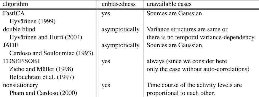
Although we concentrated on estimating functions of the form (20), we can deal with more general functions and investigate other ICA algorithms within the framework of estimating functions and asymptotic estimating functions (see also Cardoso, 1997). Such analysis helps to check whether these algorithms may give valid solutions regardless of the nuisance densities (ρz,ρV). We re-mark that our extension enables us to analyze algorithms based on temporal structure such as TD-SEP/SOBI (Ziehe and M¨uller, 1998; Belouchrani et al., 1997). Since it is quite technical, the de-tailed discussion is put in Appendix A, where the unbiasedness condition (14) of estimating func-tions is examined for these algorithms under the variance-dependent BSS model. We briefly sum-marize the consequences in Table 2. Estimators by all algorithms listed below are derived from estimating equations which satisfy the unbiasedness condition at least asymptotically. When the other conditions are taken into account, TDSEP/SOBI never works for the variance-dependent BSS model, because sources have no lagged auto-correlations. ICA algorithms using non-Gaussianity such as FastICA and JADE are not working, if sources are Gaussian. The double blind algorithm (Hyv¨arinen and Hurri, 2004) cannot be applied to the case where the variance structures of sources are the same or there is no temporal variance-dependency. The nonstationary algorithm by Pham and Cardoso (2000) is not applicable to the case where time courses of the activity levels are pro-portional to each other. Of course, such a theoretical analysis tells us only about the possibility of failure. In practice, algorithms do not always return valid answers, because of local minima and numerical instability of their learning process. Nevertheless, this theoretical analysis can explain the results of our numerical experiments in the next section.
6. Numerical Experiments
We carried out experiments with several artificial and more realistic data sets for several BSS al-gorithms. The eight batch algorithms and the online versions of the quasi maximum likelihood methods listed in Table 3 were applied to those data sets. Note that our goal is not primarily an algorithm comparison but the experiments serve to demonstrate the correctness of our theoretical analysis.
For evaluating the results, we used the index defined by Amari et al. (1996)
AmariIndex(B,A∗) = n
∑
i=1∑n
j=1|Ci j| maxk|Cik|
−1
+ n
∑
j=1∑n
i=1|Ci j| maxk|Ck j|
−1
,
algorithm unbiasedness unavailable cases
FastICA yes Sources are Gaussian.
Hyv¨arinen (1999)
double blind asymptotically Variance structures are same or
Hyv¨arinen and Hurri (2004) there is no temporal variance-dependency.
JADE asymptotically Sources are Gaussian.
Cardoso and Souloumiac (1993)
TDSEP/SOBI yes always (since we consider here
Ziehe and M¨uller (1998) only the case without auto-correlations) Belouchrani et al. (1997)
nonstationary yes Time course of the activity levels are Pham and Cardoso (2000) proportional to each other.
Table 2: Availability of other ICA and BSS algorithms
QML(tanh) quasi maximal likelihood method with the hyperbolic tangent nonlinearity QML(pow3) quasi maximal likelihood method with the cubic nonlinearity
Online(tanh) online version of QML(tanh) with learning rateη(t) = 0.1
(1+t/20)
Online(pow3) online version of QML(pow3) with learning rateη(t) = 0.25
(1+t/20)
’DoubleBlind’ the double blind algorithm by Hyv¨arinen and Hurri (2004)
JADE JADE algorithm
FastICA(tanh) FastICA with the hyperbolic tangent nonlinearity FastICA(pow3) FastICA with the cubic nonlinearity
TDSEP/SOBI TDSEP/SOBI algorithm
’Sepagaus’ The ’sepagaus’ algorithm for nonstationary signals by Pham and Cardoso (2000)
where A∗is the true mixing matrix and C=BA∗. If B=PD(A∗)−1with a permutation matrix P and a diagonal matrix D, then AmariIndex(B,A∗) =0.
6.1 Artificial Data Sets
In all artificial data sets, five source signals of various types with length T =10000 were generated and data after multiplying a random 5×5 mixing matrix were observed. We made 100 replications for each setting and compute the demixing matrix for each replication. The first data set was made according to the experiments in Hyv¨arinen and Hurri (2004). The activity levels v(t)were generated from a multivariate AR(1) model, where outliers larger than three times standard deviations from the means were reduced to these bounds. The normalized signals zi’s were i.i.d. sub-Gaussian ran-dom variables which are signed fourth-order roots of zero-mean uniform variables. The medians of the 100 replications are summarized in the row ’ar subG’ of Table 4 with the measure of deviation (3rd-quantile−1st-quantile)/2. As was pointed out by Hyv¨arinen and Hurri (2004), only ’Double-Blind’ gave small AmariIndex. Because the marginal distribution of the source signal si(t) looks like a Gaussian, all algorithms based on indices favouring non-Gaussianity failed. Even though the determinant in the left hand side of (28) is close to 0, all the assumptions are satisfied and the local consistency theorem is still valid. However, this does not directly mean that the estimated demixing matrix converges globally to the true one. In this case, many local optima can make the algorithms fail. This could also be understood from the fact that the contrast functions based on non-Gaussianity become almost flat and thus are very difficult to optimize. In the experiments, we observed that part of the true sources were often extracted correctly.
Although all the algorithms except for ’DoubleBlind’ did not work for the first difficult exam-ple, the theoretical study in principle tells that many ICA and BSS algorithms are also applicable to the variance-dependent BSS problem. So in fact the failure of the algorithms except ’Double-Blind’ can be solely explained by the particular choice of the data set which is in contrast to prior findings in Hyv¨arinen and Hurri (2004). In the second example, uniform random variables were used as zi’s instead of sub-Gaussian ones. The marginal distribution of the source signal si(t)looks Laplacian. Therefore, as was shown in the row ’ar uni’ of Table 4, the algorithms QML(tanh) and FastICA(tanh), which are suitable for super-Gaussian sources, always give correct answers. The algorithms ’DoubleBlind’, JADE and FastICA(pow3) based on 4-th order moments also worked ex-cept several failures due to outliers. We got admissible results by the nonstationary BSS algorithm ’Sepagaus’, if an appropriate smoothing window was chosen.
In the third and the fourth data, the activity levels vi(t) are sinusoidal functions with different frequencies.
vi(t) =1+0.9 sin
(13+i)πt 8000
, i=1, . . . ,5
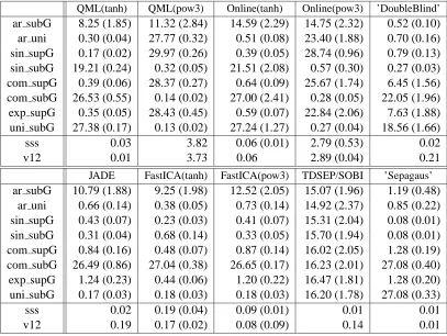
QML(tanh) QML(pow3) Online(tanh) Online(pow3) ’DoubleBlind’ ar subG 8.25 (1.85) 11.32 (2.84) 14.59 (2.29) 14.75 (2.32) 0.52 (0.10) ar uni 0.30 (0.04) 27.77 (0.32) 0.51 (0.08) 23.40 (1.88) 0.70 (0.16) sin supG 0.17 (0.02) 29.97 (0.26) 0.39 (0.05) 28.74 (0.96) 0.79 (0.13) sin subG 19.21 (0.24) 0.32 (0.05) 21.51 (2.08) 0.57 (0.30) 0.27 (0.03) com supG 0.39 (0.06) 28.37 (0.27) 0.64 (0.09) 25.67 (1.74) 6.45 (1.56) com subG 26.53 (0.55) 0.14 (0.02) 27.00 (2.41) 0.28 (0.05) 22.05 (1.96) exp supG 0.35 (0.05) 28.43 (0.45) 0.59 (0.07) 22.84 (2.06) 7.63 (1.88) uni subG 27.38 (0.17) 0.13 (0.02) 27.24 (1.27) 0.27 (0.04) 18.56 (1.66)
sss 0.03 3.82 0.06 (0.01) 2.79 (0.53) 0.02
v12 0.01 3.73 0.06 2.89 (0.04) 0.21
JADE FastICA(tanh) FastICA(pow3) TDSEP/SOBI ’Sepagaus’ ar subG 10.79 (1.88) 9.25 (1.98) 12.52 (2.05) 15.07 (1.96) 1.19 (0.48)
ar uni 0.66 (0.14) 0.38 (0.05) 0.73 (0.14) 14.92 (2.37) 0.85 (0.22) sin supG 0.43 (0.07) 0.23 (0.03) 0.41 (0.07) 15.31 (2.04) 0.08 (0.01) sin subG 0.31 (0.04) 0.68 (0.14) 0.33 (0.05) 15.70 (1.94) 0.08 (0.01) com supG 0.84 (0.16) 0.48 (0.07) 0.87 (0.14) 16.02 (2.05) 1.28 (0.19) com subG 26.49 (0.86) 27.04 (0.38) 26.65 (0.17) 16.23 (2.01) 27.08 (0.40) exp supG 1.24 (0.23) 0.44 (0.06) 1.20 (0.22) 16.47 (1.81) 1.28 (0.20) uni subG 0.17 (0.03) 0.18 (0.03) 0.18 (0.03) 16.20 (1.78) 27.08 (0.33)
sss 0.02 0.19 (0.04) 0.09 (0.01) 0.01 0.01
v12 0.19 0.17 (0.02) 0.08 (0.09) 0.14 0.01
Table 4: AmariIndex of the estimators. The values are the medians of 100 replications with the measure of deviation, (3rd-quantile−1st-quantile)/2
best performance, and all four algorithms with 4-th order moments showed better performance than the FastICA(tanh).
The double blind algorithm (’DoubleBlind’) by Hyv¨arinen and Hurri (2004) does not work when (i) all vi’s have same temporal structure, and (ii) there exist no temporal dependencies in vi’s. ’Sepagaus’ does not have a guarantee to separate sources either, because smoothed sequences of the activity levels are nearly proportional to each other (see Table 2). The fifth and sixth data set are examples of the case (i), where vi(t)are the same sinusoidal functions.
vi(t) =1+0.9 sin
πt
500
, i=1, . . . ,5
As in the third and the fourth examples, Laplace and the sub-Gaussian i.i.d. random variables were used for the normalized signals zi. As in the row ’com supG’ of Table 4, the five algorithms ex-cept QML(pow3), ’DoubleBlind’ and TDSEP/SOBI worked properly. Among them, QML(tanh) and FastICA(tanh) had better performance. ’DoubleBlind’ gave poor results, because the matrix
e
with the local consistency did not work, we carried out extra experiments with larger sample size
T . When T =200000, the AmariIndices of the estimated demixing matrices by JADE are below
0.11, 92 times out of 100 repetition. On the other hand, both FastICA methods returned valid re-sults almost always (AmariIndices are below 0.22, 89 times for FastICA(tanh) and 100 times for FastICA(pow3) ), if T =50000 and the algorithms start from the true demixing matrix. Therefore, we think that the global convergence is not achieved in these cases, because of finite sample size effects and local optima.
The seventh and the eighth data sets are examples of the case (ii), where v(t)is i.i.d. in time t. In the former example, we transform 5 independent exponential random variables linearly such that vi and vj have correlation 0.9, and zi’s were i.i.d Laplace random variables. On the other hand, in the latter example, v(t)was generated from 5 uniform random variables by the same linear transforma-tion and zi’s were the i.i.d sub-Gaussian random variables. As one can see in the row ’exp supG’ of Table 4, the results are similar to the data set ’com supG’. On the other hand, in the sub-Gaussian case summarized in the row ’uni subG’ of Table 4, QML(pow3), JADE, FastICA(tanh) and Fas-tICA(pow3) gave correct results, but ’Sepagaus’ showed very poor performance. We remark that in both cases, ’DoubleBlind’ did not work as was expected.
We would now like to digest the results from Table 4 and relate them to our theoretical find-ings. We have shown that all algorithms except for TDSEP/SOBI have the local consistency for most of the given data. However, this does not directly mean that they converge globally to the true solution. Although we hope that algorithms with a local consistency work properly, we sometimes see significant deviations from this expectation in practice as in Table 4. The algorithmic failures are caused by local optima as pointed out above for the data set ’ar subG’, or more importantly to numerical stability and convergence issues. For example, since learning algorithms like gradient descent are used for QML(tanh) and QML(pow3), desired solutions (equilibria) turn out to be in-stable for sub-Gaussian (QML(tanh)) and super-Gaussian signals (QML(pow3)). In our data sets, ’ar uni’, all data sets with ’supG’ and acoustic signals are super-Gaussian, while all data sets with ’subG’ except ’ar subG’ are sub-Gaussian. One can see the clear pattern in the columns QML(tanh) and QML(pow3). The online version Online(tanh) and Online(pow3) had slightly degraded per-formance with appropriate learning rate, if the batch version QML(tanh) and QML(pow3) worked, respectively. On the other hand, although FastICA uses similar criteria for non-Gaussianity, it em-ploys a kind of Newton’s method and so the desired solutions are automatically better stabilized. In the columns FastICA(tanh) and FastICA(pow3), except for the difficult case ’com subG’ and nearly Gaussian case ’ar subG’, both algorithms succeeded.
6.2 Variance-Dependent Speech Signals
Next we will deal with more realistic data sets. Speech and audio signals have often been used as sources s(t) even for experiments of the instantaneous ICA model. In order to check whether variance-dependency matters to many ICA and BSS algorithms, we applied BSS algorithms to speech signals which have strong variance-dependency.
In the first experiments ’sss’,8 we took two speech signals with length T =120976, where one speaker says digits from 1 to 10 in English, and the other speaker counts at the same time in Spanish. We used the separated signals of their second demo as the sources, because their separation quality is good enough. Figure 2 shows the sources and the estimators of their activity levels with
an appropriate smoother. We inserted one short pause at different positions of both sequences to make correlation of the activity levels of the modified signals much larger (0.65). In the second experiments ’v12’,9 we took two speech signals from Japanese text (T =48000). Figure 3 shows the sources and the estimators of the activity levels. We extended and shorten each syllable of the second sequence and tuned its amplitude such that the two sources have high variance-dependency. Correlation of the activity levels of the arranged signals becomes 0.74.
40000 80000 120000
2 1
40000 80000 120000
2 1
Figure 2: The sources of the data set ’sss’ and the estimators of their activity levels. The upper panel contains the signals showing counting from 1 to 10 in English and Spanish. The lower panel shows their activity levels with an appropriate smoother.
10000 20000 30000 40000
2 1
10000 20000 30000 40000
2 1
Figure 3: The sources of the data set ’v12’ and the estimators of their activity levels. The upper panel are signals from Japanese sentences. The lower panel shows their activity levels with an appropriate smoother.
A 2×2 mixing matrix A was randomly generated 100 times and 100 different mixtures of the source signals were made. The results are summarized in the rows ’sss’ and ’v12’ of Table 4. In
both experiments, QML(tanh), JADE, TDSEP/SOBI and ’Sepagaus’ always worked, while Fas-tICA(tanh) and FastICA(pow3) gave admissible results except for several cases. Although TD-SEP/SOBI is not applicable to the variance-dependent BSS model, it also returned correct results. This means that the speech signals are not perfectly matching the model Eq. (4), but the sources have furthermore a lagged autocorrelation. QML(tanh) always returned wrong answers, because speech is usually super-Gaussian.
7. Conclusions
In this paper, we discussed semiparametric estimation for blind source separation, when sources have variance dependencies. Hyv¨arinen and Hurri (2004) introduced the double blind setting where, in addition to source distributions, dependencies between components are not restricted by any parametric model. In the presence of these two nuisance parameters (densities of activity level and underlying signal), they proposed an algorithm based on lagged 4-th order cumulants. Although their algorithm works well in many cases, it fails if (i) all vi’s have similar temporal structure, or (ii) there exist no temporal dependencies in vi’s. Furthermore it also suffers from outliers.
Extending the semiparametric approach (Amari and Cardoso, 1997) under variance dependen-cies, we investigated estimating functions for the variance-dependent BSS model. In particular, we proved that the quasi maximum likelihood estimator is derived from an estimating function, and is hence consistent regardless of the true nuisance densities (which satisfy certain mild conditions). We also analyzed other ICA algorithms within the framework of (asymptotic) estimating functions and showed that many of them can separate sources with coherent variances. This is in contrast to previous understanding of the mechanisms underlying ICA algorithms. Theoretically we have shown that at least asymptotically all BSS algorithms except for TDSEP/SOBI have the local con-sistency, thus they should succeed on a given mixed data. However, local consistency does not necessarily guarantee global convergence to the true solution and we sometimes see significant de-viations from this expectation in practice. The algorithmic failures are due to many local optima and more importantly due to numerical stability and convergence issues.
Although almost all ICA and BSS algorithms could not give correct answers in the numerical experiment of Hyv¨arinen and Hurri (2004), we showed here that this was mainly a matter of the specific choice of the data set. In fact, most ICA and BSS algorithms also work well in many other benchmark examples that use dependent data. In particular, we carried out two experiments with highly variance-dependent speech signals. Despite the dependence typically found in speech, most ICA and BSS algorithms yield excellent separation results and our theoretical analysis can help to understand the reason for this fact. We conjecture that it is not the coarse amplitude structure (e.g. from dependence) that matters for BSS but the statistical fine structure of the signals.
set. We think that suitable methods might be developed along the lines of Meinecke et al. (2002) or Harmeling et al. (2004).
Acknowledgments
The authors acknowledge A. Ziehe, S. Harmeling, F. Meinecke and N. Murata for valuable discus-sions, and A. Hyv¨arinen and three anonymous reviewers for useful comments to improve this paper. We furthermore thank the PASCAL Network of Excellence (EU #506778) and DFG (SFB 618) for partial funding.
Appendix A. Comments on Other Selected BSS Algorithms
We will discuss in the following the local consistency of ICA/BSS algorithms except the quasi maximum likelihood method.
A.1 FastICA
FastICA is one of the standard algorithms for blind source separation. Let u(t) =C−1/2x(t)be the whitened data, where C= T1∑Tt=1x(t)x>(t)is the sample covariance. FastICA gives the demixing matrix W= (w1, . . . ,wn)>which maximizes the total non-Gaussianity
n
∑
i=11 T
T
∑
t=1G{w>i u(t)}
under the orthogonality condition WW>=I. We use, in the following the notation W for the demix-ing matrix after whitendemix-ing in order to distdemix-inguish it from the total demixdemix-ing matrix B=WC−1/2 including whitening process. Here G is a nonlinear function which is introduced to approximate the negentropy (Hyv¨arinen et al., 2001b). By solving the constrained optimization problem, we see that the estimator of W must satisfy the estimating equation
T
∑
t=1h
y(t)y>(t)−I+y(t)g>{y(t)} −g{y(t)}y>(t)i=0 (37)
where y(t) =W u(t). If we write the total demixing matrix as B=WC−1/2, y(t)can be expressed as Bx(t). The vector function g(y)consists of the derivatives g(yi) =G0(yi), that is, g(y) = (g(y1), . . . ,g(yn) )>. The functions (12) and (13) are also used as the function g. We remark that the equation (37) is equivalent to
T
∑
t=1h
y(t)g>{y(t)} −g{y(t)}y>(t)i = 0, (38)
T
∑
t=1h
y(t)y>(t)−I
i
because the left hand side of (38) is antisymmetric, while that of (39) is symmetric. If we determine the scales of the sources such that
E
"
T
∑
t=1{b>i x(t)}2
B,ρz,ρV #
=T, i=1, . . . ,n, (40)
then it is easy to show that the expectations of the left hand side of (38) and (39) vanish regardless of the nuisance functionsρzandρV, in the same way as for the quasi maximum likelihood method. This means that the left hand side of (37) satisfies the unbiasedness condition (14) of estimating functions. If the other regularity conditions hold, it becomes an estimating function and the esti-matorB derived from it converges to the correct demixing matrix Bb ∗= (A∗)−1with a permutation matrix P and a diagonal matrix D. Although the estimating function is similar to that of the quasi maximum likelihood, FastICA algorithm is based on the Newton’s algorithm, and therefore, it has globally more stable dynamics than the natural gradient learning.
A.2 The Double Blind Algorithm by Hyv¨arinen and Hurri (2004)
Hyv¨arinen and Hurri (2004) proposed an algorithm for separating sources under the double blind situation. The estimator is obtained by maximizing
J(W) =
∑
i,j
c
cov{y2i(·),y2j(· −∆t)}2,
under the orthogonality condition WW>=I, where
c
cov{y2i(·),y2j(· −∆t)}= 1 T−∆t
T
∑
t=∆t+1y2i(t)y2j(t−∆t)−1.
Let us assume that
d
cum{si(·),sj(·),sk(· −∆t),sl(· −∆t)}
:= 1
T−∆t T
∑
t=∆t+1si(t)sj(t)sk(t−∆t)sl(t−∆t)− 1 T2
T
∑
t=1si(t)sj(t) T
∑
t=1sk(t)sl(t)
− 1
(T−∆t)2 T
∑
t=∆t+1si(t)sk(t−∆t) T
∑
t=∆t+1sj(t)sl(t−∆t)
− 1
(T−∆t)2 T
∑
t=∆t+1si(t)sl(t−∆t) T
∑
t=∆t+1sj(t)sk(t−∆t)
=
Kik+op(1), i= j, k=l op(1), otherwise
that is, the empirical cumulants of the source signal s(t) = (A∗)−1x(t)converge to their expectation, where
Ki j= 1
T−∆t T
∑
t=∆t+1Es2i(t)s2j(t−∆t)− 1 T2
T
∑
t=1Es2i(t) T