_____________________________________________________________________________________________________ 7(3): 1-7, 2019; Article no.JERR.49875
Comparative Analysis of Rescaled Range Results of
Normal and Abnormal Heart Sound Recordings
Lotachukwu Ibe
1*and Tajudeen Abiola Ogunniyi Salau
11
Department of Mechanical Engineering, University of Ibadan, Ibadan, Nigeria.
Authors’ contributions
This work was carried out in collaboration between both authors. Author LI designed the study, performed the statistical analysis, wrote the protocol and wrote the first draft of the manuscript. Author TAOS managed the analyses of the study. Both authors read and approved the final manuscript.
Article Information DOI: 10.9734/JERR/2019/v7i316971 Editor(s): (1) Dr. P. Elangovan, Faculty of Electrical Engineering, Sri Venkateswara College of Engineering, Anna University, Chennai, India. Reviewers: (1) Nallasivan Gomathinayagam, PSN College of Engineering and Technology (Autonomous), India. (2) Francisco Bulnesm, IINAMEI, Mexico. Complete Peer review History:https://sdiarticle4.com/review-history/49875
Received 30 July 2019 Accepted 04 October 2019 Published 15 October 2019
ABSTRACT
Heart acoustics can be used as an early diagnostic tool, to quickly and accurately identify medical patients who may be at risk of unfavourable cardiovascular outcomes. However, at present, there remains no universally accepted standard or technique for detecting abnormalities using Phonocardiograms. To address this, a large database containing normal and abnormal heart sound recordings of patients were studied with the rescaled range technique and the Hurst exponent, a measure of persistence for non-linear dynamic data. Using the Hurst exponent (H) as a benchmark, we compared the values of the Hurst exponent for normal heart sound recordings with that of the abnormal heart sound recordings. For this study, the recording length was limited to the first 10 seconds for all 578 distinct recordings, which were selected randomly from the database. Furthermore, two Hurst exponent values were obtained for each recording, by subjecting them to time intervals of 1 and 2 milliseconds respectively. The results from this study show that heart sound recordings are persistent (H > 0.5) for normal and abnormal heart sound recordings, with the normal recordings being slightly more persistent.
Keywords: Hurst exponent; phonocardiogram; rescaled range; persistence; heart sound classification; cardiovascular diseases.
ABBREVIATIONS
R : Widest Spread (maximum value -
minimum value);
S : Standard deviation;
T : Study data length (Minimum allowed in
the study was 2);
H : Hurst Exponent;
K : Constant of Proportionality;
s : Seconds;
ms : Milliseconds; PCG : Phonocardiogram; ECG : Electrocardiogram; CVD : Cardiovascular Disease; MRI : Magnetic Resonance Imaging;
1. INTRODUCTION
According to the World Health Organization's 2015 report, nearly 17.5 million people died from different types of cardiovascular diseases (CVD) in the year 2012, which represents 31% of global deaths [1]. While Electrocardiograms, Computed Tomography scans and MRIs exist for the detection of CVDs, these methods are expensive in Low to Middle-Income countries (LMICs) and also require a trained hand. On the other hand, methods for automatic stratification of heart sound recordings often suffered from a lack of robustness because of the limited database available.
The 2016 PhysioNet Computing in Cardiology (CinC) Challenge addressed this issue by providing the largest dataset to date of heart sound recordings along with a common platform for the evaluation of algorithms. The data was drawn from multiple research groups across the world, recorded in various clinical and non-clinical environments [2]. Although various kinds of heart pathology exist, the challenge classifies all recordings as “normal” and “abnormal”.
Majority of the research groups that participated in the 2016 Physionet CinC Challenge attempted to classify recordings either by segmentation, feature extraction or a combination of both. Ortiz et al. [3], for example, classified Phonocardiogram (PCG) recordings by first segmenting and extracting features before using a supervised learning method. Tang et al. [4], use 324 features extracted from multi-domains of each recording to train a backpropagation neural
network for the prediction and obtain an overall score of 83.6% on the Physionet CinC performance scale. Tschannen et al. [5], developed a model that relies on a robust feature representation - generated by the wavelet-based deep convolutional neural network - of each cardiac cycle in the test recording, and support vector machine classification.
With this in mind, this paper aims to study short unsegmented PCG recordings using the rescale range technique and the Hurst exponent index to measure the degree of persistence of both classes of recordings and establish a relationship between Hurst exponent values for normal and abnormal heart sound recordings. For a more comprehensive review of prior work on heart sound classification, refer to Liu et al. [6].
2. METHODOLOGY
Three assumptions were made before
implementing the rescaled range and Hurst exponent algorithm. The first is that a valid conclusion can be made about the nature of a heart recording in 10 seconds. This was done to have a uniform recording length that is consistent with all recordings studied. Based on previous literature Nilanon et al. [7], medical practitioners concur with this assumption. Another assumption is that the behaviour of a particular recording would remain the same for a small change in the time interval. The final assumption is that heart sound recordings can be accurately studied without segmentation.
We begin this section by describing the data used in this study, then the methods used for processing the data and the final algorithm adopted.
2.1 The Dataset
Ibe and Salau; JERR, 7(3): 1-7, 2019; Article no.JERR.49875
2.2 Data Cleaning
"Noise" which is present in some of the recordings provided reduces the accuracy of the analysis used in this study and some cases prevents the execution of the rescaled range technique. As a result of this, a method of detecting and eliminating noisy signals was developed. This process is illustrated by the flowchart in the Appendix-I.
2.3 The Rescale Range Analysis
For the rescale range the method used is such that Hurst exponent is computed for each recording studied. The rescaled range depends
on the lengths of time (range) to be analysed. A recording length of 10 seconds corresponds to
a data length of 20,002. To obtain a
well-structured range, the logarithm of the size of the entire data series for each recording was divided by the logarithm of two, which yields 14.29. This value was then rounded down to its nearest whole number, after which
the new data length became two raised to the power of the rounded down number. This
gives a new data length 16,384, which is a multiple of 2 and allows for easy and consistent
division of ranges. Given the new data length of 16,384, we divided into non-overlapping
ranges of 16,384/v. With v being a multiple of 2, such that the size of each range is also an integer and 2. This yields a total of 13 distinct ranges.
The mean for each range is calculated. A series of deviations for each range was created afterwards, followed by computation of the running total of deviations from the mean.
From these values obtained, the minimum and maximum deviations, as well as the variance and standard deviation were calculated.
The rescaled range is obtained by dividing the widest spread (maximum-minimum deviations) by the Standard deviation. Since there are thirteen ranges per recording, the average rescaled range value was then computed.
2.4 The Hurst Exponent
The rescale range analysis is based on the proportional relationship between the ratio of widest spread (R) and standard deviation (S) to a power of the data length (T). As established in the literature Scheinerman, [9], the model could be represented as;
α (1)
Equation (1) can then be expressed as:
= (2)
Where K = constant of proportionality
Taking the logarithm of both sides of the equation we obtain:
Log = Log (K) + H Log (T) (3)
From equation (3), we see that the behaviour of the graph is a straight line on a log-log graph with a slope of the line being H. The interpretation of the Hurst exponent is as follows:
H = 0.5; is the Hurst exponent value for an uncorrelated time series data or a random walk.
H > 0.5; is the Hurst exponent value for a positively correlated time series (persistence).
H < 0.5; is the Hurst exponent value for a negatively correlated time series (anti-persistence).
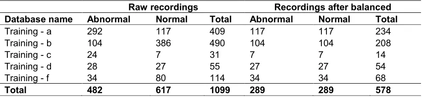
Table 1. The distribution of normal and abnormal recordings studied
Raw recordings Recordings after balanced Database name Abnormal Normal Total Abnormal Normal Total
Training - a 292 117 409 117 117 234
Training - b 104 386 490 104 104 208
Training - c 24 7 31 7 7 14
Training - d 28 27 55 27 27 54
Training - f 34 80 114 34 34 68
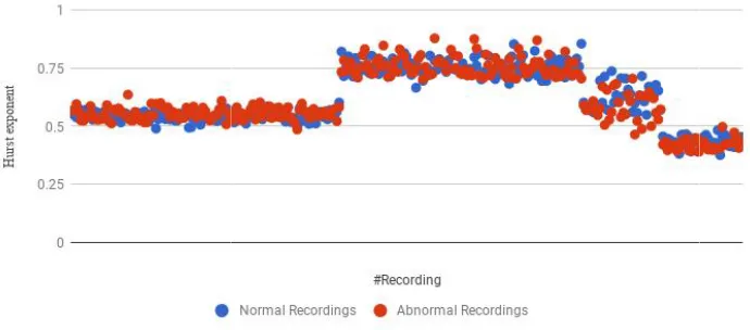
Fig. 1. Distribution of Hurst exponent values for all normal and abnormal recordings for a recording length of 1 millisecond
Fig. 2. Distribution of Hurst exponent values for
recording length of 2 milliseconds
Give adequate information to allow the experiment to be reproduced. Already published methods should be mentioned with references. Significant modifications of published methods and new methods should be described in detail. This section will include sub-sections. Tables & figures should be placed inside the text. Tables and figures should be presented as per their appearance in the text. It is suggested that the discussion about the tables and figures should appear in the text before the appearance of the respective tables and figures. No tables or figures should be given without discussion or reference inside the text.
Tables should be explanatory enough to be understandable without any text reference. Double spacing should be maintained throughout the table, including table headings and
Fig. 1. Distribution of Hurst exponent values for all normal and abnormal recordings for a recording length of 1 millisecond
Fig. 2. Distribution of Hurst exponent values for all normal and abnormal recordings for a recording length of 2 milliseconds
Give adequate information to allow the experiment to be reproduced. Already published methods should be mentioned with references. ublished methods and new methods should be described in detail. sections. Tables & figures should be placed inside the text. Tables and figures should be presented as per their appearance in the text. It is suggested that the discussion about the tables and figures should appear in the text before the appearance of the respective tables and figures. No tables or figures should be given without discussion or
Tables should be explanatory enough to be nderstandable without any text reference. Double spacing should be maintained throughout the table, including table headings and
footnotes. Table headings should be placed above the table. Footnotes should be placed below the table with superscript
letters.
3. RESULTS AND DISCUSSION
3.1 Summary Statistics for Hurst
Exponent Values
The analysis from this study are presented in the two tables and four graphs shown below; Table 2 shows the average Hurst exponent values and standard deviation for all recordings for a time intervals of 0.001 seconds and 0.002 seconds, grouped by their respective datasets. The summary of the Hurst exponents obtained for all datasets studied is presented in Table 3.
Fig. 1. Distribution of Hurst exponent values for all normal and abnormal recordings for a
all normal and abnormal recordings for a
footnotes. Table headings should be placed above the table. Footnotes should be placed below the table with superscript lowercase
SSION
Summary Statistics for Hurst
The analysis from this study are presented in the two tables and four graphs shown below; Table 2 shows the average Hurst exponent values and
Ibe and Salau; JERR, 7(3): 1-7, 2019; Article no.JERR.49875
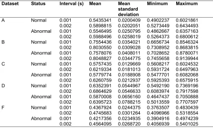
Table 2. Summary statistics of the Hurst exponents obtained for each dataset studied
Dataset Status Interval (s) Mean Mean standard deviation
Minimum Maximum
A Normal 0.001 0.5435341 0.0200409 0.4902237 0.6021861
0.002 0.5898815 0.0202051 0.5273449 0.6434493
Abnormal 0.001 0.5546495 0.0250795 0.4862667 0.6357163
0.002 0.5988496 0.0258019 0.5264373 0.6800612
B Normal 0.001 0.7554436 0.0354021 0.6656734 0.8546324
0.002 0.8030550 0.0309028 0.7308952 0.8683815
Abnormal 0.001 0.7578076 0.0408011 0.7028652 0.8780071
0.002 0.8048827 0.0344775 0.7455658 0.9139944
C Normal 0.001 0.5757435 0.0129669 0.5608217 0.6024532
0.002 0.6219334 0.0181013 0.5931724 0.6497963
Abnormal 0.001 0.5779774 0.0188908 0.5477701 0.6082068
0.002 0.6260759 0.0212937 0.5925393 0.6575915
D Normal 0.001 0.6352391 0.0544967 0.5492190 0.7369196
0.002 0.6864629 0.0546633 0.6083974 0.7917598
Abnormal 0.001 0.5870008 0.0656160 0.4647437 0.7050888
0.002 0.6395723 0.0788215 0.5013559 0.7707597
F Normal 0.001 0.4367924 0.0244375 0.3763507 0.4830439
0.002 0.4745683 0.0301264 0.4096966 0.5318554
Abnormal 0.001 0.4217356 0.0234935 0.3904916 0.4974239
0.002 0.4564095 0.0268720 0.4056939 0.5401025
Table 3. The average Hurst exponent values for all normal and abnormal heart sound recordings for time intervals of 0.001 seconds and 0.002 seconds
Time Interval = 0.001 seconds Time Interval = 0.002 seconds Status Mean Standard Deviation Mean Standard Deviation Abnormal heart
recording
0.61570881 0.12111164 0.66069933 0.12411861
Normal heart recording
0.61658211 0.11819548 0.66282773 0.12010887
It is observed from Table 3 that the Hurst exponents for both normal and abnormal recordings (0.001 seconds) are both greater than 0.5, that is, H > 0.5, with the values ranging from 0.61570881 (Abnormal heart recording) to 0.61658211 (Normal Heart recording). This implies that both the normal and the abnormal heart recordings on average exhibit persistence. In more detail, the implication of these values for their Hurst exponents is that, a high signal measured by the digital Phonocardiogram is likely to be followed by another high signal in the short period, and that this property, by inference is common to both the abnormal and normal heart recordings.
Similarly, from Table 3; it is observed that the Hurst exponents for both normal and abnormal recordings (0.002 seconds) are both greater than 0.5, that is, H > 0.5, with the values ranging from 0.66069933 (Abnormal heart recordings) to
0.6628773 (Normal Heart recordings). This implies that both the normal and the abnormal heart recordings also exhibit persistence for a time interval of 0.002 seconds.
From Table 3, the following can be inferred:
1. The average Hurst exponent values for an abnormal heart recording measured with an interval of 0.001 seconds (standard) can be written as 0.61570881 (+ or - 0.12111164).
2. The average Hurst exponent values for a normal heart recording measured with an interval of 0.001 seconds (standard) can be written as 0.61658211 (+ or - 0.11819548).
4. The average Hurst exponent values for an abnormal heart recording measured with an interval of 0.002 seconds can be written as 0.66282773 (+ or - 0.12010887).
The percentage of persistent correlation for the normal and abnormal recordings is expressed below:
1. Percentage persistent correlation for an abnormal heart recording measured with a time interval of 0.001 seconds: (0.61570881 - 0.5) / 0.5 = 0.23141762 (23.14%).
2. Percentage persistent correlation for a normal heart recording measured with a time interval of 0.001 seconds: (0.61658211 - 0.5) / 0.5 = 0.23316422 (23.32%).
3. Percentage persistent correlation for an Abnormal heart recording measured with a time interval of 0.002 seconds: (0.66069933-0.5)/ 0.5 = 0.32139866 (32.14%).
4. Percentage persistent correlation for a normal heart recording measured with a time interval of 0.002 seconds: (0.66282773-0.5)/ 0.5 = 0.32565546 (32.57%).
4. CONCLUSION
In this work, normal and abnormal heart sound recordings have been studied comparatively using a robust non-linear technique. Normal and Abnormal heart sound recordings are persistent in the time intervals studied, which implies that forecasting is possible for both classes of heart recordings. Concerning their index of dependence, we conclude that both classes of recordings behave in a quasi-similar fashion.
ACKNOWLEDGEMENTS
The authors are grateful to the Mechanical Engineering Department of the University of Ibadan for supporting this paper with useful resources. We would also like to the organizers of the 2016 Physionet CinC Challenge for providing the large dataset that was used in this study.
COMPETING INTERESTS
Authors have declared that no competing interests exist.
REFERENCES
1. World Health Organization. World statistics on cardiovascular disease; 2015.
(Accessed February 2018)
Available:https://who.int/mediacentre/facts heets/fs317/en/
2. Clifford GD, Liu CY, Moody B, Springer D, Silva I, Li Q, et al. Classification of normal/abnormal heart sound recordings. The physionet/computing in cardiology challenge. Computing in Cardiology. 2016;43(2):154-79
3. Ortiz JJG, Phoo CP, Wiens J. Heart sound classification based on temporal alignment techniques. Computing in Cardiology Conference (CinC). 2016;43: 589-92.
4. Tang H, Chen H, Li T, Zhong M. Classification of normal/abnormal heart sound recordings based on multi-domain features and backpropagation neural network. Computing in Cardiology Conference (CinC). 2016;43:593-96. 5. Tschannen M, Kramer T, Marti G,
Heinzmann M, Wiatowski T. Heart sound classification using deep structured features. Computing in Cardiology Conference (CinC). 2016;43:565–68 6. Liu C, Springer D, Li Q, Moody B, Juan
RA, Chorro FJ, et al. An open-access database for the evaluation of heart sound algorithm. Physiological Measurement. 2016;37(12):218-213.
7. Nilanon T, Yao J, Hao J, Purushotham S, Liu. Normal/abnormal heart sound recordings classification using a convolutional neural network. Computing in Cardiology Conference (CinC). 2016;43:585-88.
8. Goldberger AL, Amaral LAN, Glass L, Hausdorff JM, Ivanov PCh, Mark RG.
PhysioBank, PhysioToolkit, and
PhysioNet: Components of a new research resource for complex physiologic signals. Circulation. 2000;101(23):215-20.
[Circulation Electronic Pages].
Available:http://circ.ahajournals.org/cgi/con tent/full/101/23/e215
Ibe and Salau; JERR, 7(3): 1-7, 2019; Article no.JERR.49875
APPENDIX I
Flow chart for data cleaning
© 2019 Ibe and Salau; This is an Open Access article distributed under the terms of the Creative Commons Attribution License (http://creativecommons.org/licenses/by/4.0), which permits unrestricted use, distribution, and reproduction in any medium, provided the original work is properly cited.
Peer-review history: