Minimax Regret Classifier for Imprecise Class Distributions
Roc´ıo Alaiz-Rodr´ıguez [email protected]
Dpto. de Ingenier´ıa El´ectrica y de Sistemas y Autom ´atica Campus de Vegazana, Universidad de Le ´on
24071 Le´on, Spain
Alicia Guerrero-Curieses [email protected]
Dpto. de Teor´ıa de la Se˜nal y Comunicaciones
Campus de Fuenlabrada, Universidad Rey Juan Carlos Camino del Molino s/n, 28943 Fuenlabrada-Madrid, Spain
Jes ´us Cid-Sueiro [email protected]
Dpto. de Tecnolog´ıas de las Comunicaciones EPS, Universidad Carlos III de Madrid
Avda. de la Universidad, 30, 28919 Legan´es-Madrid, Spain
Editor: Dale Schuurmans
Abstract
The design of a minimum risk classifier based on data usually stems from the stationarity assump-tion that the condiassump-tions during training and test are the same: the misclassificaassump-tion costs assumed during training must be in agreement with real costs, and the same statistical process must have generated both training and test data. Unfortunately, in real world applications, these assumptions may not hold. This paper deals with the problem of training a classifier when prior probabilities cannot be reliably induced from training data. Some strategies based on optimizing the worst pos-sible case (conventional minimax) have been proposed previously in the literature, but they may achieve a robust classification at the expense of a severe performance degradation. In this paper we propose a minimax regret (minimax deviation) approach, that seeks to minimize the maximum devi-ation from the performance of the optimal risk classifier. A neural-based minimax regret classifier for general multi-class decision problems is presented. Experimental results show its robustness and the advantages in relation to other approaches.
Keywords: classification, imprecise class distribution, minimax regret, minimax deviation, neural
networks
1. Introduction - Problem Motivation
prior probabilities and the misclassification costs) may be non representative of the underlying real distributions.
If the ratio of training data corresponding to each class is not in agreement with real class distributions, designing Bayes decision rules based on prior probabilities estimated from these data will be suboptimal and can seriously affect the reliability and performance of the classifier.
A similar problem may arise if real misclassification costs are unknown during training. How-ever, they are usually known by the end user, who can adapt the classifier decision rules to cost changes without re-training the classifier. For this reason, our attention in this paper is mainly focused on the problem of uncertainty in prior probabilities. Furthermore, being aware that class distribution is seldom known (at least totally) in real world applications, a robust approach (as op-posite to adaptive) that prevents severe performance degradation appears to be convenient for these situations.
Besides other adaptive and robust approaches that address this problem (discussed in more detail in Section 2.2) it is important to highlight those that handle the problem of uncertainty in priors by following a robust minimax principle: minimize the maximum possible risk. Analytic foundations of minimax classification are widely considered in the literature (see VanTrees, 1968; Moon and Stirling, 2000; Duda et al., 2001, for instance) and a few algorithms to carry out minimax decisions have been proposed. From computationally expensive ones such as estimating probability density functions (Takimoto and Warmuth, 2000; Kim, 1996) or using methods from optimization (Polak, 1997) to simpler ones like neural network training algorithms (Guerrero-Curieses et al., 2004; Alaiz-Rodriguez et al., 2005).
Minimax classifiers may, however, be seen as over-conservative since its goal is to optimize the performance under the least favorable conditions. Consider, for instance, a direct marketing campaign application carried out in order to maximize profits. Since optimal decisions rely on the proportion of potential buyers and it is usually unknown in advance, our classification system should take into account this uncertainty. Nevertheless, following a pure minimax strategy can lead to solutions where minimizing the maximum loss implies considering there are no potential clients. If it is the case, this minimax approach does not seem to be suitable for this kind of situation.
In this imprecise class distribution scenario, it can be noticed that the classifier performance may be highly deviated from the optimal, that is, that of the classifier knowing actual priors. Minimizing this gap (that is, the maximum possible deviation with respect to the optimal classifier) is the focus of this paper. We seek for a system as robust as the conventional minimax approach but less pessimistic at the same time. We will refer to it as a minimax deviation (or minimax regret) classifier. In contrast to other robust and adaptive approaches, it can be used in general multiclass problems. Furthermore, as shown in Guerrero-Curieses et al. (2004), minimax approaches can be used in combination with the adaptive proposal by Saerens et al. (2002) to exploit its advantages.
This minimax regret approach has recently been applied in the context of parameter estimation (Eldar et al., 2004; Eldar and Merhav, 2004) and a similar competitive strategy has been used in the context of hypothesis testing (Feder and Merhav, 2002).
This paper is organized as follows: the next section provides an overview of the problem as well as some previous approaches to cope with it. Next, Section 3 states the fundamentals of minimax classification together with a deeper analysis of the minimax regret approach proposed in this pa-per. Section 4 presents a neural training algorithm to get a neural-based minimax regret classifier under complete uncertainty. Moreover, practical situations with partial uncertainty in priors are also discussed. A learning algorithm to solve them is provided in Section 5. In Section 6, some experi-mental results show that minimax regret classifiers outperform (in terms of maximum risk deviation) classifiers trained on re-balanced data sets and those with the originally assumed priors. Finally, the main conclusions are summarized in Section 7.
2. Problem Overview
Traditionally, supervised learning lies in the fact that training data and real data come from the same (although unknown) statistical model. In order to carefully analyze to what extend classifier per-formance depends on conditions such as class distribution or decision costs, learning and decision theory principles are briefly revisited. Next, some previous approaches to deal with environment imprecision are reviewed.
2.1 Learning and Making Optimal Decisions
Let S={(xk,dk),k=1, . . . ,K}denote a set of labelled samples where xk∈RNis an observation fea-ture vector and dk∈UL={u0, . . . ,uL−1}is the label vector. Class-i label uiis a unit L-dimensional vector with components ui,j =δi j, with every component equal to 0, except the i-th component which is equal to 1.
We assume a learning process that estimates parameters w of a non-linear mapping fw:RN→
P
from the input space into probability space
P
={p∈[0,1]L|∑L−1i=0 pi=1}. The soft decision is given by yk=fw(xk)∈
P
and the hard output of the classifier is denoted bybd. Note that d andbd will beused to distinguish the actual class from the predicted one, respectively.
Several costs (or benefits) associated with each possible decision are also defined: ci j denotes the cost of deciding in favor of class i when the true class is j. Negative values represent benefits (for instance, cii, which is the cost of correctly classifying a sample from class i could be negative in some practical cases).
In general cost-sensitive classification problems, either misclassification costs ci jor ciicosts can take different values for each class. Thus, there are many applications where classification errors lead to very different consequences (medical diagnosis, fault detection, credit risk analysis), what implies misclassification costs ci j that may largely vary between them. In the same way, there are also many domains where correct decision costs (or benefits) ciido not take the same value. For instance, in targeted marketing applications (Zadrozny and Elkan, 2001), correctly identifying a buyer implies some benefit while correctly classifying a non buyer means no income. The same applies to medical diagnosis domains such as the gastric carcinoma problem studied in G ¨uvenir et al. (2004). In this case, the benefit of correct classification also depends on the class: the benefit of correctly classifying an early stage tumor is higher than that of a later stage.
The expected risk (or loss) R is given by
R =
L−1
∑
j=0 L−1
∑
i=0
where P{bd=ui|d=uj}with i6= j represent conditional error probabilities, and Pj=P{d=uj}is the prior probability of class uj.
Defining the conditional risk of misclassifying samples from class uj as
Rj= L−1
∑
i=0
ci jP{bd=ui|d=uj} ,
we can express risk (1) as
R=
L−1
∑
i=0
RiPi . (2)
It is well-known that the Bayes decision rule for the minimum risk is given by
b
d=arg min
ui { L−1
∑
j=0
ci jP{d=uj|x}} , (3)
where P{d=ui|x}is the a posteriori probability of class i given sample x.
The optimal decision rule depends on posterior probabilities and therefore, on the prior proba-bilities and the likelihood.
In theory, as long as posterior probabilities (or likelihood and prior probabilities) are known, the optimal decision in Eq. (3) can be expressed after a trivial manipulation as a function of the cost differences between the costs (ci j−cj j) (Duda et al., 2001). This is the reason why cj j is usually assumed to be zero and the value of the cost difference is directly assigned to ci j. When dealing with practical applications, however, some authors (Zadrozny and Elkan, 2001; G ¨uvenir et al., 2004) have urged to use meaningful decision costs measured over a common baseline (and not necessarily taking cj j=0) in order to avoid mistakes that otherwise could be overlooked. For this reason and, what is more important, the uncertainty class distribution problem addressed in this paper, decision costs measured over a common baseline are considered. Furthermore, absolute values of decision costs are relevant to the design of classifiers under the minimax regret approach.
2.2 Related Work: Dealing with Cost and Prior Uncertainty
Most proposals to address uncertainty in priors fall into the categories of adaptive and robust solu-tions. While the aim of a robust solution is to avoid a classifier with very poor performance under any conditions, an adaptive system pursues to fit the classifier parameters using more incoming data or more precise information.
With an adaptive-oriented principle, Provost (2000) states that, once the classifier is trained under specific class distributions and cost assumptions (not necessarily the operating conditions), the selection of the optimal classifier for specific conditions is carried out by a correct placement of the decision thresholds. In the same way, the approaches in Kelly et al. (1999) and Kubat et al. (1998) consider that tuning the classifier parameters should be left to the end user, expecting that class distributions and misclassification costs will be precisely known then.
them when precise information about priors or costs is available. Under imprecision, some classi-fiers can be discarded but this does not necessarily provide a method to select the optimal classifier between the possible ones and fit its parameters. Furthermore, due to its graphical character, these methods are limited to binary classification problems.
Changes in prior probabilities have also been discussed by Saerens et al. (2002), who proposes a method based on re-estimating the prior probabilities of real data in an unsupervised way and subse-quently adjusting the outputs of the classifier according to the new apriori probabilities. Obviously, the method requires enough unlabelled data being available for re-estimation.
As an alternative to adaptive schemes, several robust solutions have been proposed, as the re-sampling methods, especially in domains where imbalanced classes come out (Kubat and Matwin, 1997; Lawrence et al., 1998; Chawla et al., 2002; Barandela et al., 2003). Either by undersampling or oversampling, the common purpose is to balance artificially the training data set in order to get a uniform class distribution, which is supposed to be the least biased towards any class and, thus, the most robust against changes in class distributions.
The same approach is followed in cost sensitive domains, but with some subtle differences in practice. It is well known that class priors and decision costs are intrinsically related. For instance, different decision costs can be simulated by altering the priors and vice versa (see Ting, 2002, for instance). Thus, when a uniform distribution is desired in a cost sensitive domain, but working with cost insensitive decision machines, class priors are altered according to decision costs, what is commonly referred as rebalancing.
The manipulation of the training data distribution has been applied to cost-sensitive learning in two-class problems (Breiman et al., 1984) in the following way: basically, the class with higher misclassification cost (suppose n times the lowest misclassification cost) is represented with n times more examples than the other class. Besides random sampling strategies, other sampling-based re-balancing schemes have been proposed to accomplish this task, like those considering closeness to the boundaries between classes (Japkowicz and Stephen, 2002; Zhou and LiuJ, 2006) or the cost-proportionate rejection sampling presented in Zadrozny et al. (2003). Extending the formulation of this type of procedures to general multiclass problems with multiple (and possibly asymmetric) inter-class misclassification costs appears to be a nontrivial task (Zadrozny et al., 2003; Zhou and LiuJ, 2006), but some progress has been made recently with regard to this latter point (Abe et al., 2004). Note, also, that many (although not all) of these rebalancing strategies are usually imple-mented by oversampling and/or subsampling, that is, replicating examples (without adding any extra information) and/or deleting them (which implies information loss).
3. Robust Classifiers Under Prior Uncertainty: Minimax Classifiers
Prior probability uncertainty can be coped from a robust point of view following a minimax derived strategy. Minimax regret criterion is discussed in this section after presenting the conventional minimax criterion.
Although our approach extends to general multi-class problems and the discussion is carried out in that way, we will first illustrate, for the sake of clarity and simplicity, a binary situation.
3.1 Minimax Classifiers
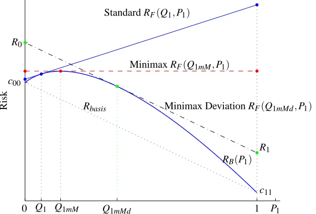
distributions (frequency for each class) give rise to different Bayes classifiers. Fig. 1 shows the Bayes risk curve, RB(P1)versus class-1 prior probability for a binary classification problem.
PSfrag replacements
c11
R1
Minimax RF(Q1mM,P1)
Standard RF(Q1,P1)
Minimax Deviation RF(Q1mMd,P1)
RB(P1)
Risk Rbasis
0 Q1 Q1mM Q1mMd 1 P1
c00
R0
Figure 1: Risk vs. P1. Minimum risk curve and performance under prior changes for the standard, minimax and minimax deviation classifier. RB(P1) stands for the optimal Bayes Risk against P1. RF(Q1,P1)denotes the Risk of a standard classifier (Fixed decision rule opti-mized for prior probabilities Q1estimated in the training phase) against P1. RF(Q1mM,P1) denotes the Risk of a minimax classifier (Fixed decision rule optimized for the minimax probabilities Q1mM) against P1. RF(Q1mMd,P1) denotes the Risk of a minimax deviation classifier (Fixed decision rule optimized for the minimax deviation probabilities Q1mMd) against P1.
If the prior probability distribution is unknown when the classifier is designed, or this distribu-tion changes with time or from one environment to other, the mismatch between training and test conditions can degrade significantly the classifier performance.
For instance, assume that Q= (Q0,Q1)is the vector with class-0 and class-1 prior probabilities estimated in the training phase, respectively, and let RB(Q1)represent the minimum (Bayes) risk attainable by any decision rule for these priors. Note, that, according to Eq. (2), for a given classifier, the risk is a linear function of priors. Thus, risk RF(Q1,P1) associated to the (fixed) classifier optimized for Q changes linearly with actual prior probabilities P1 and P0 =1−P1, going from
(0,R0) to(1,R1) (the continuous line in Fig. 1), where R0 and R1 refer to the class conditional risks for classes 0 and 1, respectively. Fig. 1 shows the impact of this change in priors and how performance deviates from optimal.
The dashed line in Fig. 1 shows the performance of the minimax classifier, which minimizes the maximum possible risk under the least favorable priors, thus providing the most robust solution, in the sense that performance becomes independent from priors. From Fig. 1, it becomes clear that the minimax classifier is optimal for prior probabilities P=QmM= (Q0mM,Q1mM)maximizing RB. Thus, this strategy is equivalent to maximizing the minimum risk (Moon and Stirling, 2000; Duda et al., 2001). We will refer to them as the minimax probabilities.
Fig. 1 also makes clear that although a minimax classifier is a robust solution to address the imprecision in priors, it may become a somewhat pessimistic approach.
3.2 Minimax Deviation Classifiers
We propose an alternative classifier that, instead of minimizing the maximum risk, minimizes the maximum deviation (regret) from the optimal Bayes classifier. In the following, we will refer to it as the minimax deviation or minimax regret classifier.
A comparison between minimax and minimax deviation approaches is also shown in Fig. 1. This latter case corresponds to a classifier trained on prior probabilities P=QmMdwith performance as
a function of priors given by a line (a plane or hyperplane for three or more classes, respectively) parallel to what we name, in the following, basis risk (Rbasis=c00(1−P1) +c11P1).
Note that the maximum deviation (with respect to priors) of the classifier optimized for Q is given by
D(Q) =max P1 {
RF(Q1,P1)−RB(P1)}=max{R0−c00,R1−c11} .
The inspection of Fig. 1 shows that the minimum of D (with respect to Q) is achieved when
R0−c00=R1−c11 ,
which means that line RF(Q1,P1) is parallel to arc named Rbasis in the figure and tangent to RB at Q1mMd. Therefore, the minimax regret classifier is also the Bayes solution with respect to the least favorable priors(Q0mMd,Q1mMd)(see Berger, 1985, for instance), which will be denoted as minimax deviation probabilities.
Now, we extend the formulation to a general L-class problem.
Definition 1 Consider a L-class decision problem with costs ci j,0≤i,j<L and cj j≤ci j, and let Rw(P)be the risk of a decision machine with parameter vector w when prior class probabilities are
given by P= (P0, . . . ,PL−1). The deviation function is defined as Dw(P) =Rw(P)−RB(P)
and the minimax deviation is defined as
DmMd=inf
w maxP {Dw(P)} . (4)
Note that the above definition assumes that the maximum exists. This is actually the case, since Dw(P)is a linear function over a compact set,
P
. Note, also, that our definition includes the naturalassumption that cj j is never higher than ci j, meaning that making a decision error is always less costly than taking the correct decision. This assumption is used in part of our theoretical analysis.
Theorem 2 The minimax deviation is given by
DmMd=inf
w maxP {Dw(P)} ,
where
Dw(P) =Rw(P)−Rbasis(P) (5)
and
Rbasis(P) = L−1
∑
j=0
cj jPj . (6)
Proof Note that, according to Eqs. (1) and (2), for any decision machine and any ui∈
U
L,R(uj) =Rj= L−1
∑
i=0
ci jP{bd=ui|d=uj} ≥cj j .
Since the bound is reached by the classifier deciding bd=uj for any observation x, we have RB(uj) =cj j. Therefore, using Eq. (6), we find that, for any u∈
U
L,RB(u) =Rbasis(u)
and, thus,
Dw(u) =Dw(u) .
Since Bayes minimum risk RB(P)is a convex function of priors and Rw(P)is linear, Dw(P)is
concave and, thus, it is maximum at some of the vertices in
P
(i.e., at some P=u∈U
L). Thus,max
P {Dw(P)}=umax∈UL{
Dw(u)} . (7)
Since the maximum difference between two hyperplanes defined over
P
is always at some vertex, we can conclude thatmax
P {Dw(P)}=umax∈UL{
Dw(u)}=max u∈UL{
Dw(u)} . (8)
Combining Eqs. (4), (7) and (8), we get
DmMd=inf
w maxP {Dw(P)} .
Note that Rbasisrepresents the risk baseline of the ideal classifier with zero errors. Th. 2 shows that the minimax regret can be computed as the minimax deviation to this ideal classifier. Note, also, that if costs ciido not depend on i, Eq. (5) becomes equivalent (up to a constant) to the Bayes risk and the minimax regret classifier becomes equivalent to the minimax classifier .
Theorem 3 Consider the minimum deviation function given by
Dmin(P) =inf
w{Dw(P)} , (9)
where Dw(P)is the normalized deviation function given by Eq. (5), and let P∗be the prior
proba-bility vector providing the maximum deviation,
P∗=arg max
P
Dmin(P) . (10)
If Dmin(P) is continuously differentiable at P=P∗, then the minimax deviation, DmMd, defined by Eq. (4), is
DmMd=Dmin(P∗) =max
P infw
Dw(P) . (11)
Proof
For any classifier with parameter vector w, we can write,
max
P Dw(P)≥Dw(P
∗)≥D min(P∗) and, thus,
inf
w maxP Dw(P)≥Dmin(P
∗) . (12)
Therefore, Dmin(P∗)is a lower bound of the minimax regret.
Now we prove that Dmin(P∗)is also an upper bound. According to Eq. (9), for anyε>0, there exists a parameter vector wεsuch that
Dwε(P∗)≤Dmin(P∗) +ε . (13) By definition, for any P, Dmin(P)≤Dwε(P). Therefore, using Eq. (13), we can write
Dwε(P∗)−Dwε(P)≤Dmin(P∗)−Dmin(P) +ε . (14) Since Dmin(P)is continuously differentiable and (according to Eq. (10)) maximum at P∗, for any ε0>0 there existsδ>0 such that, for any P∈
P
withkP∗−Pk ≤δwe haveDmin(P∗)−Dmin(P)≤ε0kP∗−Pk ≤ε0δ . (15) Let Pδa prior such thatkP∗−Pδk=δ. Takingε=ε0δand combining Eqs. (14) and (15) we can write
Dwε(P∗)−Dwε(Pδ)≤2ε0δ .
Since the above condition is verified for anyε0>0 and any prior Pδat distanceδfrom P, and taking into account that Dwε(P)is a linear function of P, we conclude that the maximum slope of Dwε(P) is bounded by 2ε0and, thus, for any P∈
P
, we haveDwε(P)−Dwε(P∗)≤2ε0kP−P∗k ≤2 √
2ε0 ,
(where we have used the fact that the maximum distance between two probability vectors is √2). Therefore, we can write
max
P Dwε(P)≤Dwε(P
and, thus,
inf
w maxP Dw(P)≤Dwε(P
∗) +2√2ε0 .
Finally, using Eq. (13) and taking into account thatε=ε0δ≤√2ε0we get
inf
w maxP Dw(P)≤Dmin(P
∗) +3√2ε0 . (16)
Since the above is true for anyε0>0 we conclude that Dmin(P∗) is also an upper bound of Dw.
Therefore, combining Eqs. (12) and (16), we conclude that
inf
w maxP Dw(P) =Dmin(P
∗) ,
which completes the proof.
Note that the deviation function needs to be neither differentiable nor a continuous function of w parameters.
If the minimum deviation function is not continuously differentiable at the minimax deviation probability, P∗, the theorem cannot be applied. The reason is that, although there should exist at least one classifier providing the minimum deviation at P=P∗, it or they could not provide a constant deviation with respect to the prior probability. The situation can be illustrated with an example.
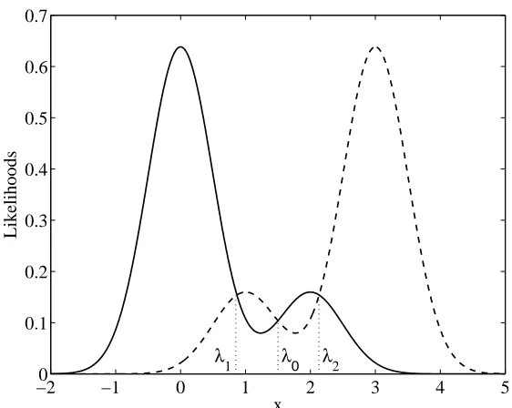
Let x∈Rbe given by p(x|d=0) =0.8N(x,σ) +0.2N(x−2,σ)and p(x|d=1) =0.2N(x− 1,σ) +0.8N(x−3,σ), whereσ=0.5 and N(x,σ) = (2πσ)−1/2exp(−x2/(2σ2)), and consider the setΦλof classifiers given by a single threshold over x and decision
ˆ d=
1 if x≥λ 0 if x<λ.
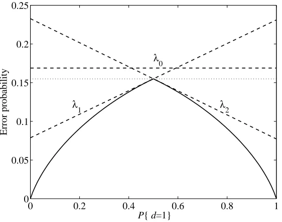
Fig. 2 shows the distribution of both classes over x, and Fig. 3 shows, as a function of priors, the minimum error probability (continuous line) that can be obtained using classifiers inΦλ. Note that decision costs c00=c11=0 and c01=c10=1 have been considered for this illustrative problem. An abrupt slope change is observed at the minimax deviation probability, for P{d=1}=1/2. For this prior, there are two single threshold classifiers providing the minimum error probability, which are given by thresholdsλ1andλ2in Fig. 2. However, as shown in Fig. 3 neither of them provides a risk that is constant in the prior. The minimax deviation classifier inΦλ, which has a thresholdλ0, does not attain minimum risk at the minimax deviation probability and, thus, cannot be obtained by using Eq. (11).
For this example, the desired robust classifier should have a deviation function given by the horizontal dotted line in Fig. 3. Fortunately, it can be obtained by combining the outputs of several classifiers. For instance, let ˆd1 and ˆd2 the decisions of classifiers given by thresholdsλ1 andλ2, respectively. It is not difficult to see that the classifier selecting ˆd1and ˆd2at random (for each input sample x) provides a robust classifier.
This procedure can be extended to the multiclass-case: consider a set of L classifiers with pa-rameters wk, k=0, . . . ,L−1, and consider the classifier such that, for any input sample x, makes a decision equal todbk(i.e., the decision of classifier with parameters wk), with probability qk. It is not difficult to show that the deviation function of this classifier is given by
D(P) =
L−1
∑
j=0 Pj
L−1
∑
k=0
qkDj(wk)
!
−20 −1 0 1 2 3 4 5 0.1
0.2 0.3 0.4 0.5 0.6 0.7
x
Likelihoods
λ1 λ0 λ2
Figure 2: The conditional data distributions for the one-dimensional example discussed in the text. λ1andλ2are the thresholds providing the minimum risk at the minimax deviation prob-ability.λ0provides the minimax deviation classifier.
where Dj(wk) =Rj(wk)−cj j. In order to get a constant deviation function, probabilities qkshould be chosen in such a way that
L−1
∑
k=0
qkDj(wk) =D ,
where D is a constant. Solving these linear equations for qk, k=0, . . . ,L−1 (with the constraint ∑kqk=1), the required probabilities can be found.
Note that, in order to build the non-deterministic classifier providing a constant deviation, a set of L independent classifiers that are optimal at the minimax deviation prior should be found. However, we go no further on the investigation of this special case for two main reasons:
• The situation does not seem to be common in practice. In our simulations, we have found that the maximum of the minimum risk deviation always provided a response which is approxi-mately parallel to Rbasis.
• In general, the abrupt change in the derivative may be a symptom that the classifier struc-ture is not optimal for the data distribution. Instead of building a nondeterministic classifier, increasing the classifier complexity should be more efficient.
0 0.2 0.4 0.6 0.8 1 0
0.05 0.1 0.15 0.2 0.25
P{ d=1}
Error probability
λ1 λ2
λ
0
Figure 3: Error probabilities as a function of prior probability of class 1 for the example in Fig. 2. Thresholdsλ1andλ2do not provide the minimax deviation classifier, which is obtained for thresholdλ0. However, the random combination of classifiers with thresholdsλ1and λ2(dotted line) provides a robust classifier with deviation lower than that ofλ0.
we must incorporate the estimation of the least favorable prior in the learning process. Next, we propose a training algorithm in order to get a minimax regret classifier based on neural networks.
4. Neural Robust Classifiers Under Complete Uncertainty
Note that, if QmMd is the probability vector providing the maximum in Eq. (11), that is,
QmMd=arg max
P
n
inf
w{Dw(P)}
o
,
then we can write
DmMd=inf
w{Dw(QmMd)} .
4.1 Updating Network Weights
Learning is based on minimizing some empirical estimate of the overall error function
E{C(y,d)}=
L−1
∑
i=0
P{d=ui}E{C(y,d)|d=ui}= L−1
∑
i=0 PiCi ,
where C(y,d)may be any error function and Ciis the expected conditional error for class-i. Selecting the appropriate error function (see Cid-Sueiro and Figueiras-Vidal, 2001, for in-stance), learning rules can be designed providing a posteriori probability estimates (yi≈P{d= ui|x}, where yi is the soft decision) and, thus, according to Eq. (3), the hard decision minimizing the risk can be approximated by
b
d=arg min i {
L−1
∑
j=0
ci jyj} .
The overall empirical error function (cost function) used in learning for priorsbP= (Pb0, . . . ,PbL−1) may be written as
b
C =
L−1
∑
i=0
b
PiCbi= L−1
∑
i=0
b Pi 1 Ki K
∑
k=1
dikCb(yk,dk),
= 1
K
"L
−1
∑
i=0
b
Pi Ki/K
K
∑
k=1
dikC(yk,dk)
!# , = 1 K K
∑
k=1
"L
−1
∑
i=0
b
Pi
b
Pi(0)
dikCb(yk,dk)
#
, (17)
wherePbi(0)=Ki/K is an initial estimate of class-i prior based on class frequencies in the training set andPbiis the current prior estimate.
Minimizing error function (17) by means of a stochastic gradient descent learning rule leads to update the network weights at k-th iteration as
w(k+1) = w(k)−µ L−1
∑
i=0
b
Pi(n)
b
Pi(0)
dik∇wC(yk,dk)
,
= w(k)− L−1
∑
i=0
µ(in)dik∇wC(yk,dk) , (18)
where
µ(in)=µPb (n) i
b
Pi(0)
(19)
is a learning step scaled by the prior ratio. Note that di selects the appropriate µ( n)
4.2 Updating Prior Probabilities
Eq. (11) shows that the learning process should maximize (5) with respect to the prior probabilities. The estimate of (5) can be computed as
b¯
Dw(P) =Rbw(P)−Rbasis(P) , (20)
where
b
Rw(P) =
L−1
∑
j=0
b
RjPj (21)
is the overall Bayes risk estimate and
b
Rj= 1 Nj
L−1
∑
i=0
ci jNi j (22)
is the class- j conditional risk estimate where Nj is the number of class uj patterns in the training phase and Ni jis the number of samples from class ujassigned to ui.
In order to derive a learning rule to find an estimate Pbi satisfying constraints∑Li=−01Pbi=1 and 0≤Pbi≤1, we will use auxiliary variables Bisuch that
b
Pi=
exp(Bi) ∑L−1
j=0exp(Bj)
. (23)
We maximizeDb¯wwith respect to Bi. Applying the chain rule,
∂Db¯w ∂Bi
=
L−1
∑
j=0 ∂Db¯w
∂Pbj ∂Pbj ∂Bi
,
and using Eqs. (20), (21) and (23), we get
∂Db¯w ∂Bi
=
L−1
∑
j=0
(Rbj−cj j)Pbi(δi j−Pbj),
= Pbi Rbi−cii− L−1
∑
j=0
(RbjPbj) + L−1
∑
j=0
(cj jPbj)
!
,
= Pbi
b
Ri−cii
−Rbw−Rbbasis
,
= PbiRbdi ,
where
b
Rdi= (Rbi−cii)−(Rbw−Rbbasis) .
The learning rule for auxiliary variable Biis
Bi(n+1) = B(in)+ρ ∂Dbw
∂Bi
,
where parameterρ>0 controls the rate of convergence. Using Eq. (23) and Eq. (24), the updated learning rule forPbiis
b
Pi(n+1) =
exp(B(in))expρPbi(n)Rb(din)
∑L−1 j=0
h
expB(jn)expρPb(jn)Rb(d jn)i
,
=
b
Pi(n)expρPbi(n)Rb(din)
∑L−1 j=0
h b
P(jn)expρPb(jn)Rb(d jn)i
. (25)
4.3 Training Algorithm for a Minimax Deviation Classifier
In the previous section, both the network weights updating rule (18) and the prior probability update rule (25) have been derived. The algorithm resulting from the combination is shown as follows:
for n=0 to Niterations−1 do for k=1 to K do
w(k+1)=w(k)− L−1
∑
i=0
µ(in)dik∇wC(yk,dk)
end for
EstimateRb(n),Rbi(n), i=0, . . . ,L−1, according to (21) and (22)
Update minimax probabilityPbi(n+1), i=0, . . . ,L−1 according to (25) and compute µ(in+1)with (19)
end for
5. Robust Classifiers Under Partial Uncertainty
Although in many practical situations prior probabilities may not be specified with precision, they can be partially known. In this section we discuss how partial information about priors can be used to improve the classifier performance in relation to a complete uncertainty situation.
From now on, let us consider that lower (or upper) bounds of the priors are known based on previous experience. We will denote the lower and upper bounds of class-i prior probability as Pil and Piu, respectively.
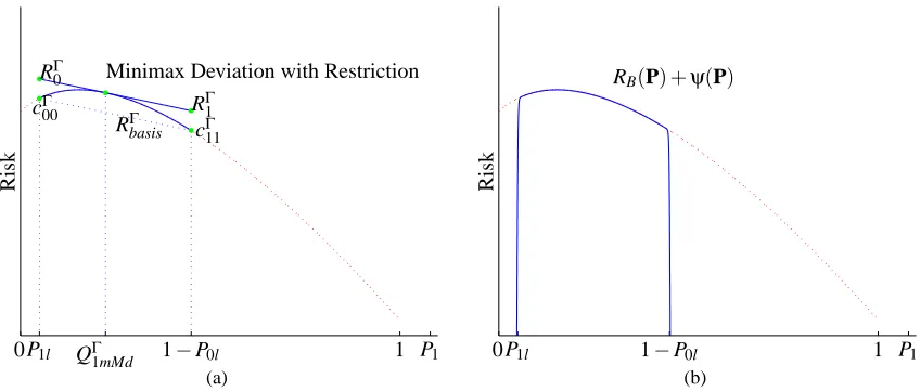
In order to illustrate this situation consider a binary classification problem where probability lower bounds P0land P1lare known. That is, P1∈[P1l,1−P0l]where this interval represents the un-certainty region. Let us denote byΓ={P : 0≤Pi≤1,∑Li=−01Pi=1,Pi≥Pil}the probability region satisfying the imposed constraints. In the following, we will refer toΓas the uncertainty region.
ALAIZ-RODR´IGUEZ, GUERRERO-CURIESES,ANDCID-SUEIRO
RΓ0
RΓ1 RΓbasis cΓ00
cΓ11
Minimax Deviation with Restriction
Risk
0P1l QΓ1mMd 1−P0l 1 P1 0
0.5 1 1.5 2 2.5 3 3.5
(a)
PSfrag replacements
Risk
RB(P) +ψ(P)
0P1l 1−P0l 1 P1
(b)
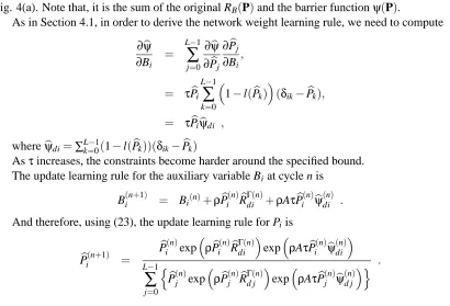
Figure 4: Minimax deviation classifier under partial uncertainty of prior probabilities: (a)Γ-minMaxDev Classifier. (b) Modified cost function defined as RB(P) +ψ(P).
In contrast to the minimax regret criterion, note that a classical minimax classifier for the con-sidered uncertainty region would minimize the worst-case risk. It would be a Bayes solution for the prior where the minimum risk reaches its maximum and it could be denoted as QΓmM.
Notice, also, that these solutions will be the same if the risk for the vertex ofΓtake the same value (cΓii=k).
5.1 Neural Robust Classifiers Under Partial Uncertainty
Minimax search can be formulated as maximizing (with respect to priors) the minimum (with re-spect to network parameters) of deviation function (5), as described in previous section, but subject to some constraints
arg max
P infw {D
Γ
w(P)} ,
s.t. Pi≥Pil, i=0, . . . ,L−1
where DΓw=RΓw−RΓbasis. When uncertainty is global, this hyperplane is defined by the risk in the L extreme cases with Pi=δik, that is, by the corresponding cii. However, with partial knowledge of
the prior probabilities, this hyperplane becomes defined by the risk in L points which are the vertex given by the restrictions and with associated risk denoted by cΓj j.
Defining
l(Pi) =
1
1+exp−τ(Pi−Pil) , (26) whereτcontrols the hardness of this restriction, the minimax problem can be re-formulated as
arg max
P infw {D
Γ
w(P)}
s.t. l(Pi)≥1/2, i=0, . . . ,L−1.
arg max
P infw {D
Γ
w(P) +Aψ(P)} ,
whereψ(Pi) =log(l(Pi))and the constant A determines the contribution of the barrier function. Fig. 4(b) shows the new risk function corresponding to the binary case previously depicted in Fig. 4(a). Note that, it is the sum of the original RB(P)and the barrier functionψ(P).
As in Section 4.1, in order to derive the network weight learning rule, we need to compute
∂ψb
∂Bi
=
L−1
∑
j=0 ∂ψb
∂Pbj ∂Pbj ∂Bi
,
= τPbi L−1
∑
k=0
1−l(Pbk)
(δik−Pbk),
= τPbiψdib ,
whereψdib =∑Lk=−01(1−l(Pbk))(δik−Pbk)
Asτincreases, the constraints become harder around the specified bound. The update learning rule for the auxiliary variable Biat cycle n is
B(in+1) = Bi(n)+ρPb( n) i Rb
Γ(n)
di +ρAτPb (n) i ψb
(n) di .
And therefore, using (23), the update learning rule for Pi is
b
Pi(n+1) =
b
Pi(n)expρPbi(n)RbdiΓ(n)expρAτPbi(n)ψb(din)
L−1
∑
j=0
n b
P(jn)expρPb(jn)Rbd jΓ(n)expρAτPbj(n)ψb(d jn)o
.
Note that if the upper bound is known instead of the lower bound, l(Pi)defined by (26) should be replaced by u(Pi) = (1+exp(τ(Pi−Piu)))−1at the previous formulation.
The minimax constrained optimization problem has been tackled by considering a new objective function defined by the sum of the original cost function and a barrier function. Studying the convexity of this new function becomes important from the fact that a stationary point of this risk curve is a global maximum.
Since the minimum risk curve (RB(P)) is a convex function of the priors (see VanTrees, 1968, for details), if we verify the convexity of the barrier function, we can conclude that the function defined by the sum of both of them is also convex.
This barrier function is convex in
P
if the Hessian matrix HRverifies PTHRP≤0The Hessian matrix of the barrier function equals to a diagonal matrix Dr=diag(r) with all
negative diagonal entries ri=Aτ2(−l(Pi)(1−l(Pi))). As l(Pi)∈[0,1]and therefore, ri ≤0, it is straightforward to see that
PTHRP = PTDrP,
=
L−1
∑
i=0
Pi2ri≤0 .
5.2 Extension to Other Learning Algorithms
The learning algorithm proposed in this paper is intended to train a minimax deviation classifier based on neural networks with feedforward architecture. Actually, the learning algorithm we pro-pose becomes a feasible solution for any learning process based on minimizing some empirical estimate of an overall cost (error) function.
However, it is also applicable to a general classifier provided it is trained (in an iterative process) for the estimated minimax deviation probabilities and the assumed decision costs. Specifically, in this paper, scaling the learning rate allows to simulate different class distributions and the hard decisions are made based on posterior probability estimates and decision costs. Furthermore, the neural learning phase carried out in one iteration can be re-used for the next one, what allows to reduce computational cost with respect to a complete optimization process on each iteration. Apart from the general approach of completely training a classifier on each iteration and in order to reduce its computational cost, specific solutions may be studied for different learning machines. Nonetheless, it seems not feasible to readily achieve this improvement for classifiers like SVMs, where support vectors for one solution may have nothing in common with the ones obtained in next iteration and thus, making necessary to re-train the classifier in each iteration.
Another possible solution for any classifier that provides a posteriori probabilities estimates or any score that can be converted into probabilities (for details on calibration methods see Wei et al., 1999; Zadrozny and Elkan, 2002; Niculescu-Mizil and Caruana, 2005) is outlined here. In this case, an iterative procedure able to estimate the minimax deviation probabilities and consequently to adjust (without re-training) the outputs of the classifier could be studied. The general idea for this approach is as follows: first, the new minimax deviation prior probabilities are estimated according to (25) and then, posterior probabilities provided by the model are adjusted as follows (see Saerens et al., 2002, for more details)
P(k){d=ui|x}=
Pi(k)
Pi(k−1)P
(k−1){d=ui|x}
L−1
∑
j=0 P(jk)
P(jk−1)
P(k−1){d=uj|x}
. (27)
The algorithm’s main structure is summarized as for k=1 to K do
EstimateRb(k),Rbi(k), i=0, . . . ,L−1, according to (21), (22) and decision costs ci j Update minimax probabilityPbi(k+1)according to (25)
Adjust classifier outputs according to (27) end for
6. Experimental Results
In this section, we first present the neural network architecture used in the experiments and illustrate the proposed minimax deviation strategy on an artificial data set. Then, we apply it to several real-world classification problems. Moreover, a comparison with other proposals such as the traditional minimax and the common re-balancing approach is carried out.
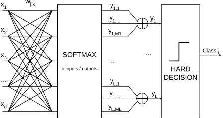
6.1 Softmax-based Network
Although our algorithms can be applied to any classifier architecture, we have chosen a neural network based on the softmax non-linearity with soft decisions given by
yi= Mi
∑
j=1 yi j ,
with
yi j=
exp(wT
i jx+wi j0) ∑L−1
k=0∑ Mk
l=1exp(wTklx+wkl0)
,
where L stands for the number of classes, Mjthe number of softmax outputs used to compute yjand wi j are weight vectors. We will refer to this network as a Generalized Softmax Perceptron(GSP).1 A simple network with Mj=2 is used in the experiments.
... SOFTMAX
n inputs / outputs
wj,k
x1
x2
x3
xd
...
... y1,1
y1,M1
yL,1
yL,ML
y1,...
yL,...
HARD DECISION
Class i
y1
yL
Figure 5: GSP(Generalized Softmax Perceptron) Network
Fig. 5 corresponds to the neural network architecture used to classify the samples represented by feature vector x. Learning consists of estimating network parameters w by means of the stochastic gradient minimization of certain objective functions. In the experiments, we have considered the Cross Entropy objective function given by
CE(y,d) =−
L
∑
i=1
dilog yi .
The stochastic gradient learning rule for the GSP network is given by Eq. (18). Learning step µ(k)decreases according to µ(k)= 1+µ(k/0)η ,where k is the iteration number, µ(0)the initial learning rate andηa decay factor.
The reason to illustrate this approach with a feedforward architecture is that, as mentioned in Section 5.2, it allows to exploit (in the iterative learning process) the partially optimized solution in current iteration for the next one. On the other hand, posterior probability estimation makes it possible to apply the adaptive strategy based on prior re-estimation proposed by Saerens to the min-imax deviation classifier, as long as a data set representative of the operation conditions is available. Finally, the fact that intermediate outputs yi jof the GSP can be interpreted as subclass probabilities may provide quite a natural way to cope with the unexplored problem of uncertainty in subclass distributions as already pointed out by Webb and Ting (2005). Nonetheless, both architecture and cost function issues are not the goal of this paper, but merely illustrative tools.
6.2 Artificial Data Set
To illustrate the minimax regret approach proposed in this paper both under complete and partial uncertainty, an artificial data set with two classes (class u0and class u1) has been created. Data ex-amples are drawn from the normal distribution p(x|d=ui) =N(mi,σ2i) with mean miand standard deviationσi. Mean values were set to m0=0, m1=2 and standard deviation toσ0=σ1=√2. A to-tal of 4000 instances were generated with prior probabilities of class membership P{d=u0}=0.93 and P{d=u1}=0.07. The cost-benefit matrix
c00 c01 c10 c11
is given by
2 5 4 0
.
Initial learning rate was set to µ(0)=0.3, decay factor toη=2000 and training was ended after 80 cycles. Classifier assessment was carried out by following 10-fold cross-validation.
Two classifiers were trained, to be called a standard classifier and a minMaxDev classifier. The former is built by considering that the estimated class prior information is precise and stationary and the latter is the approach proposed in this paper to cope with uncertainty in priors. Thus, for the standard classifier, its performance may deviate from the optimal risk in 3.39 when priors change from training to test conditions. However, a minimax deviation classifier reduces this worst-case difference from the optimal classifier to 0.77.
Now, we suppose that some information about priors is available (partial uncertainty). For instance, we consider that the lower bound for prior probabilities P0 and P1 are known and set to P0l =0.55 and P1l =0.05, respectively, so that the uncertainty region is Γ={(P0,P1)|P0 ∈
[0.55,0.95],P1∈[0.05,0.45]}.
A minimax deviation classifier can be derived for Γ (it will be called Γ-minMaxDev classi-fier).The narrowerΓis, the closer the minimax deviation classifier performance is to the optimal. For this particular case, under partially imprecise priors, the standard classifier may differ from optimal (inΓ) in 0.83, while the use of the simple minMaxDev classifier designed under total prior uncertainty conditions attains a maximum deviation of 0.53. However, theΓ-minMaxDev classifier only differs from optimal in 0.24. These data are reported in Table 1 where both, experimental and also theoretical results, are shown.
6.3 Real Databases
Classifier
Standard minMaxDev Γ-minMaxDev Th/Exp Th/Exp Th/Exp Maximum deviation from optimal
(complete uncertainty) 3.41/3.39 0.72/0.77 – Maximum deviation from optimal inΓ
(partial uncertainty) 0.85/0.83 0.50/0.53 0.19/0.24
Table 1: A comparison between the standard classifier (build under stationary prior assumptions), the minimax deviation classifier (minMaxDev) and the minimax deviation classifier under partial uncertainty (Γ-minMaxDev) for an artificial data set
Database # Classes Class distribution # Attributes # Instances
German Credits (GCRE) 2 [0.70 0.30] 8 1000
Australian Credits (AUS) 2 [0.32 0.68] 14 690
Munich Credits (MCRE) 2 [0.30 0.70] 20 1000
Insurance Company (COIL) 2 [0.94 0.06] 85 9822
DNA Slice-junction (DNA) 3 [0.24 0.24 0.52] 180 3186
Page-blocks (PAG) 5 [0.90 0.06 0.01 0.01 0.02] 10 5473
Dermatology (DER) 6 [0.31 0.16 0.20 0.13 0.14 0.06] 34 366 Pen-digits (PEN) 10 [0.104 0.104 0.104 0.096 0.104
0.096 0.096 0.104 0.096 0.096]
16 10992
Table 2: Experimental Data sets
Other public data set used is Munich Credits from the Dept. of Statistics at the University of Mu-nich.2
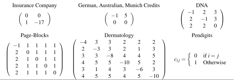
Data set description is summarized in Table 2, and cost-benefit matrices are shown in Table 3. We have used the cost values that appear in Ikizler (2002) for those data sets in common. Otherwise, for lack of an expert analyst, the cost values have been chosen by hand.
2. Data sets available at http://www.stat.uni-muenchen.de/service/datenarchiv/welcome e.html.
Insurance Company German, Australian, Munich Credits DNA
0 0
1 −17
−1 5
0 0
−
1 2 3
2 −1 3
2 2 0
Page-Blocks Dermatology Pendigits
−1 1 1 1 1
2 0 1 1 1
2 1 0 1 1
2 1 1 0 1
2 1 1 1 0
−4 3 3 2 2 2
2 −3 3 2 1 3
3 3 −8 4 4 5
4 5 5 −10 5 2
3 1 4 3 −6 3
4 5 5 4 5 −10
ci j=
0 if i=j 1 Otherwise
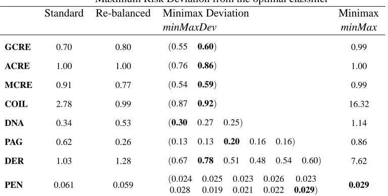
Maximum Risk Deviation from the optimal classifier
Standard Re-balanced Minimax Deviation Minimax
minMaxDev minMax
GCRE 0.70 0.80 (0.55 0.60) 0.99
ACRE 1.00 1.00 (0.76 0.86) 1.00
MCRE 0.91 0.77 (0.54 0.59) 0.99
COIL 2.78 0.99 (0.87 0.92) 16.32
DNA 0.34 0.53 (0.30 0.27 0.25) 1.14
PAG 0.62 0.26 (0.13 0.13 0.20 0.16 0.16) 0.86
DER 1.03 1.28 (0.67 0.78 0.51 0.48 0.54 0.60) 7.62
PEN 0.061 0.059 (0.024 0.025 0.023 0.026 0.023
0.028 0.019 0.021 0.022 0.029) 0.029
Table 4: Classifier Performance evaluated as Maximum Risk Deviation from the optimal classifier for several real-world applications. Class-conditional risk deviations (Ri−cii) reported for the minMaxDev classifier.
Experimental results for these data sets are shown in the following sections. The robustness of different decision machines under complete uncertainty of prior probabilities is analyzed in Section 6.3.1. If uncertainty is only partial, a similar study and comparison with the previous approach (complete uncertainty) is carried out in Section 6.3.2.
6.3.1 CLASSIFIERROBUSTNESSUNDERCOMPLETEUNCERTAINTY
We now study how different neural-based classifiers cope with worst-case situations in prior prob-abilities. The maximum deviation from the optimal classifier (see Table 4) is reported for the pro-posed minMaxDev strategy as well as for other alternative approaches: the one based on the as-sumption of stationary priors (standard) and the common alternative of deriving the classifier from an equally distributed data set (re-balanced). A comparison with the traditional minimax strategy is also provided. Together with the previously mentioned value (maximum deviation or regret), deviation for the L class-conditional extreme cases (Ri−cii) is also reported for the minMaxDev classifier in Table 4. Results allow to verify that this solution is fairly close to the optimal one where deviation is not dependent on priors and thus, class-conditional deviations take the same value.
Although the balanced class distribution to train the classifier can be obtained by means of undersampling and/or oversampling, it is simulated by altering the learning rate used in the training
phase according to (19) as µi=µ 1/L
b
Pi(0)
,where 1/L represents the simulated probability, equal for
all classes.
Maximum Risk
Standard Re-balanced Minimax Deviation Minimax
minMaxDev minMax
GCRE 0.70 0.15 0.60 0.00
ACRE 0.01 0.02 0.86 -0.00
MCRE 0.05 0.20 0.59 0.00
COIL 0.76 0.99 0.86 0.02
DNA 0.34 0.53 0.25 0.13
PAG 0.62 0.26 0.20 0.10
DER -2.10 -1.68 -2.21 -2.38
PEN 0.061 0.059 0.029 0.029
Table 5: Classifier Performance measured as Maximum Risk for several real-world applications.
standard classifier while this reduces to 0.20 for the minMaxDev one. Likewise, for the Insurance company(COIL) application the maximum deviation for the standard classifier is 2.78 compared with 0.92 for the minMaxDev model. The remaining databases also show the same behavior as it is presented in Table 4.
On the other hand, the use of a classifier inferred from a re-balanced data set does not necessarily involve a decrease in the maximum deviation with respect to the standard classifier. In the same way, the traditional minimax classifier does not protect against prior changes in terms of maximum relative deviation from the minimum risk classifier.
However, if our criterion is more conservative and our aim is the minimization of the maximum possible risk (not the minimization of the deviation), the traditional minimax classifier represents the best option. It is shown in Table 5 where the maximum risk for the different classifiers is reported. Positive values in this table indicate a cost while negative values represent a benefit. For instance, for the Page-blocks application the minimax classifier assures a maximum risk of 0.10 while the standard, re-balanced and minMaxDev classifiers reach values of 0.62, 0.26 and 0.20, respectively. It can be noticed that for the Pen-digits data set, the minimax deviation and minimax approaches attain the same results. The reason is that, for this problem, the Rbasisplane takes the same value (in this case, zero) in the probability space.
6.3.2 CLASSIFIERROBUSTNESS UNDER PARTIALUNCERTAINTY
Unlike the previous section, we consider now that partial information about the class priors is avail-able. The aim is to find a classifier that behaves well for a delimited and realistic range of priors what constitutes an aid in reducing the maximum deviation from the optimal classifier. This situ-ation can be treated as a constrained minimax regret strategy where the constraints represent any extra information about prior probability value.
Lower bound for prior probabilities
Data Set P0l P1l P2l P3l P4l P5l P6l P7l P8l P9l
GCRE 0.40 0.25
ACRE 0.20 0.25
MCRE 0.20 0.25
COIL 0.15 0.03
DNA 0.10 0.10 0.25
PAG 0.22 0.02 0.00 0.01 0.02
DER 0.1 0.20 0.10 0.10 0.10 0.02
PEN 0.10 0.06 0.06 0.10 0.10 0.06 0.06 0.10 0.05 0.05
Table 6: Lower bounds for prior probabilities defining the uncertainty region,Γregion for the ex-perimental data sets.
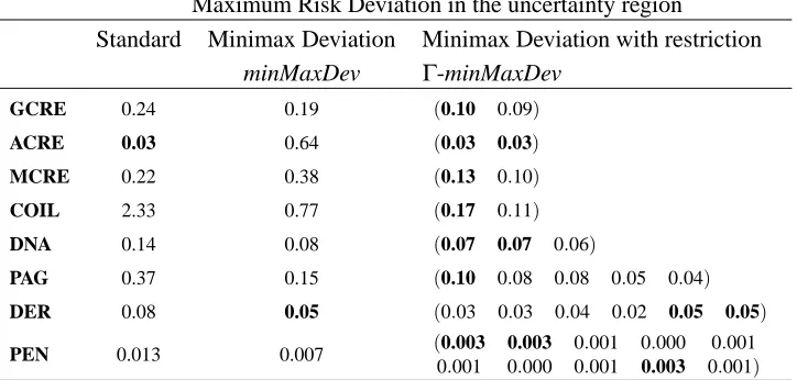
Maximum Risk Deviation in the uncertainty region
Standard Minimax Deviation Minimax Deviation with restriction minMaxDev Γ-minMaxDev
GCRE 0.24 0.19 (0.10 0.09)
ACRE 0.03 0.64 (0.03 0.03)
MCRE 0.22 0.38 (0.13 0.10)
COIL 2.33 0.77 (0.17 0.11)
DNA 0.14 0.08 (0.07 0.07 0.06)
PAG 0.37 0.15 (0.10 0.08 0.08 0.05 0.04)
DER 0.08 0.05 (0.03 0.03 0.04 0.02 0.05 0.05)
PEN 0.013 0.007 (0.003 0.003 0.001 0.000 0.001
0.001 0.000 0.001 0.003 0.001)
Table 7: Classifier Performance under partial knowledge of prior probabilities measured as Maxi-mum Risk Deviation for several real-world applications. Class-conditional risk deviations (RΓi −cΓii) are reported for theΓ-minMaxDev classifier.
Maximum deviation from the optimal inΓis reported for theΓ-minMaxDev classifier together with the standard and the minMaxDev ones. For instance, the standard classifier for the Page-blocks data set deviates from the optimal classifier, in the defined uncertainty region, up to 0.37, while when complete uncertainty is assumed the maximum deviation is equal to 0.62.
7. Conclusions
This work concerns the design of robust neural-based classifiers when the prior probabilities of the classes are partially or completely unknown, even by the end user.
This problem of uncertainty in the class priors is often ignored in supervised classification, even though it is a widespread situation in real world applications. As a result, the reliability of the inducted classifier can be greatly affected as previously shown by the experiments.
To tackle this problem, we have proposed a novel minimax deviation strategy with the goal to minimize the maximum deviation with respect to the optimal classifier.
A neural network training algorithm based on learning rate scaling has been developed. The experimental results show that this minimax deviation (minMaxDev) classifier protects against prior changes while other approaches like ignoring this uncertainty or use a balanced learning data set may result in large differences in performance with respect to the minimum risk classifier. Also, it has been shown that the conventional minimax classifier reduces the maximum possible risk following a conservative attitude but at the expense of large worst-case differences from the optimal classifier.
Furthermore, a constrained minimax deviation approach (Γ-minMaxDev) has been derived for those situations where uncertainty is only partial. This may be seen as a general approach with some particular cases: a) precise knowledge of prior probabilities and b) complete uncertainty about the priors. In a) the region of uncertainty collapses to a point and we have the Bayes’ rule of minimum risk and in b) the pure minimax deviation strategy comes up. While the first one may be criticized for being quite unrealistic, the other may be seen rather pessimistic. The experimental results for this proposed intermediate situation show that the Γ-minMaxDev classifier allows to reduce the maximum deviation from the optimal and performs well over a range of prior probabilities.
Acknowledgments
The authors thank the four referees and the associate editor for their helpful comments. This work was partially supported by the project TEC2005-06766-C03-02 from the Spanish Ministry of Education and Science.
References
N. Abe, B. Zadrozny, and J. Langford. An iterative method for multi-class cost-sensitive learning. In Proceedings of the Tenth ACM SIGKDD International Conference on Knowledge Discovery and Data Mining, pages 3–11, 2004.
N. M. Adams and D. J. Hand. Comparing classifiers when the misallocation costs are uncertain. Pattern Recognition, 32(7):1139–1147, March 1998.
R. Alaiz-Rodriguez, A. Guerrero-Curieses, and J. Cid-Sueiro. Minimax classifiers based on neural networks. Pattern Recognition, 38(1):29–39, January 2005.
R. Barandela, J. S. Sanchez, V. Garc´ıa, and E. Rangel. Strategies for learning in class imbalance problems. Pattern Recognition, 36(3):849–851, March 2003.
C. L. Blake and C. J. Merz. UCI repository of machine learning databases, 1998. URL http://www.ics.uci.edu/ mlearn/MLRepository.html.
L. Breiman, J. H. Friedman, R. A. Olshen, and C. J. Stone. Classification and Regression Trees. Chapman & Hall, NY, 1984.
N. V. Chawla, K. W. Bowyer, L. O. Hall, and W. P. Kegelmeyer. Smote: Synthetic minority over-sampling technique. Journal of Artificial Intelligence Research, 16:321–357, 2002.
J. Cid-Sueiro and A. R. Figueiras-Vidal. On the structure of strict sense Bayesian cost functions and its applications. IEEE Transactions on Neural Networks, 12(3):445–455, May 2001.
C. Drummond and R. C. Holte. Explicitly representing expected cost: An alternative to ROC rep-resentation. In Proceedings of the Sixth ACM SIGKDD International Conference on Knowledge Discovery and Data Mining, pages 198–207. ACM Press, 2000.
R. O. Duda, P. E. Hart, and D. G. Stork. Pattern Classification. John Wiley and Sons, 2001.
Y. C. Eldar and N. Merhav. Minimax approach to robust estimation of random parameters. IEEE Trans. on Signal Processing, 52(7):1931–1946, July 2004.
Y. C. Eldar, A. Ben-Tal, and A. Nemirovski. Linear minimax regret estimation of deterministic parameters with bounded data uncertainties. IEEE Trans. on Signal Processing, 52(8):2177– 2188, August 2004.
M. Feder and N. Merhav. Universal composite hypothesis testing: A competitive minimax approach. IEEE Trans. on Information Theory, 48(6):1504–1517, June 2002.
A. Guerrero-Curieses, R. Alaiz-Rodriguez, and J. Cid-Sueiro. A fixed-point algorithm to minimax learning with neural networks. IEEE Transactions on Systems, Man and Cybernetics Part C, 34 (4):383–392, November 2004.
H. A. G¨uvenir, N. Emeksiz, N. Ikizler, and N. ¨Ormeci. Diagnosis of gastric carcinoma by classifi-cation on feature projections. Artificial Intelligence in Medicine, 31(3), 2004.
N. Ikizler. Benefit maximizing classification using feature intervals. Technical Report BU-CE-0208, Bilkent University, Ankara, Turkey, 2002.
N. Japkowicz and S. Stephen. The class imbalance problem: A systematic study. Intelligent Data Analysis Journal, 6(5):429–450, November 2002.
M. G. Kelly, D. J. Hand, and N. M. Adams. The impact of changing populations on classifier performance. In Proceedings of Fifth International Conference on SIG Knowledge Discovery and Data Mining (SIGKDD), pages 367–371, San Diego, CA, 1999.
H. J. Kim. On a constrained optimal rule for classification with unknown prior individual group membership. Journal of Multivariate Analysis, 59(2):166–186, November 1996.