An Anticorrelation Kernel for Subsystem Training in
Multiple Classifier Systems
Luciana Ferrer∗ [email protected]
Speech Technology and Research Laboratory SRI International
333 Ravenswood Ave
Menlo Park, California, 94025, USA
Kemal S¨onmez [email protected]
Division of Biomedical Computer Science, School of Medicine Oregon Health and Science University
3181 S.W. Sam Jackson Park Rd. Portland, Oregon, 97239, USA
Elizabeth Shriberg [email protected]
Speech Technology and Research Laboratory SRI International
333 Ravenswood Ave
Menlo Park, California, 94025, USA
Editor: Leon Bottou
Abstract
We present a method for training support vector machine (SVM)-based classification systems for combination with other classification systems designed for the same task. Ideally, a new system should be designed such that, when combined with existing systems, the resulting performance is optimized. We present a simple model for this problem and use the understanding gained from this analysis to propose a method to achieve better combination performance when training SVM systems. We include a regularization term in the SVM objective function that aims to reduce the average class-conditional covariance between the resulting scores and the scores produced by the existing systems, introducing a trade-off between such covariance and the system’s individual performance. That is, the new system “takes one for the team”, falling somewhat short of its best possible performance in order to increase the diversity of the ensemble. We report results on the NIST 2005 and 2006 speaker recognition evaluations (SREs) for a variety of subsystems. We show a gain of 19% on the equal error rate (EER) of a combination of four systems when applying the proposed method with respect to the performance obtained when the four systems are trained independently of each other.
Keywords: system combination, ensemble diversity, multiple classifier systems, support vector machines, speaker recognition, kernel methods
1. Introduction
The work presented in this paper is motivated by our work on the task of speaker verification. In the last decade, many successful speaker verification systems have relied on the combination of various component systems to achieve superior performance. In many cases, as in Ferrer et al. (2006) and Brummer et al. (2007), the combination leads to significant improvements. However, there are cases in which combining several comparably good systems does not result in improvements over the single best system (Reynolds et al., 2005). Most of these systems perform the combination of information sources at the score level1 (Reynolds et al., 2003; Ferrer et al., 2006; Brummer et al., 2007; Huenup´an et al., 2007; Dehak et al., 2007): systems that model each type of feature using a certain model are independently developed and their scores are combined to produce the final score and the decision. When training each individual system, all other systems available for combination are usually ignored while, in fact, the ultimate goal of the systems is to perform well in combination with all the other systems and not necessarily individually.
It is easy to see that system combination at the score level is not guaranteed to give strictly better performance than those of the individual systems being combined. In the extreme case, if all classifiers were generating exactly the same output for each sample, the combined classifier would not have better performance than the individual ones, independently of the combination procedure used. Intuitively, what we wish is to have enough diversity across systems such that classifiers contribute complementary information leading to a better final decision when systems are combined. System diversity has been the subject of a large amount of research in recent years, with two main goals: defining a measure of diversity that can predict the performance of the combination, and designing procedures for achieving diversity in an ensemble of systems. With the goal of motivating and placing our work in perspective, in the next section we present a discussion focused on existing techniques for measuring and designing for system diversity.
The contributions of this paper are: (1) the development of a simple model for the combination problem for a binary classification task under the assumption that the distribution of scores for each of the classes is Gaussian, and (2) a procedure for improving diversity in an ensemble including SVM classifiers. We find an upper bound on the EER of an ensemble combination and show that, for a two-system combination, this upper bound is a function of the performance of the individ-ual systems and the correlation coefficient obtained from the average class-conditional covariance matrix of the scores from the two systems. Based on this result, we propose the inclusion of a regularization term in the SVM objective function when training a new SVM system for combina-tion with a set of preexisting systems, which introduces a trade-off between the performance of the resulting model and its average class-conditional covariance with the preexisting systems. Ferrer et al. (2008b) presented empirical results using the proposed method. Here, we extend this previous work by developing a framework under which to understand the method, considering the cases of multiple preexisting systems and nonlinear kernels, and including new results on simulated and on the NIST 2005 and 2006 speaker-verification evaluation data. Results show that a gain of 19% on EER can be achieved when using the proposed method with respect to the results obtained when systems are trained without knowledge of the others.
The paper is organized as follows. Section 2 gives a review of the related research. Section 3 describes a simple model for the system combination problem under consideration. Using the
conclusions obtained from this development, Section 4 proposes a method for achieving improved combination performance. In Sections 5 and 6 we present results on simulated data and speaker verification data, respectively. Section 7 presents our conclusions.
2. Multiple Classifier Systems
In this section we review the literature related to our work, motivating and putting in perspective the research presented in the rest of the paper.
2.1 Measuring Diversity
For regression problems, the measures of ensemble diversity are well developed. Krogh and Vedelsby (1995) showed that the quadratic error for a certain input value of a convex combination of estima-tors trained on a single data set is guaranteed to be less than or equal to the weighted average quadratic error of the component estimators. The difference between the two is given by an am-biguity term that measures the variability among ensemble members for the particular input. On a related development, Ueda and Nakano (1996) give a decomposition of the mean square error of an ensemble classifier into three terms: average bias, variance and covariance of the ensemble mem-bers. One would then wish to reduce the covariance term without affecting the bias and variance terms by reducing the correlation between the members. This term can, in fact, be negative.
combination weights. This problem is solved explicitly for the case of unbiased and uncorrelated estimation errors.
Two assumptions made by Tumer and Ghosh, as well as Fumera and Roli, are not well suited for the problem of interest in this paper but can be easily replaced for other assumptions without much consequence on the theory: the use of the classification error as measure of performance and the uncorrelatedness of the estimation errors across classes. Classification error is usually considered inappropriate for problems in which the prior probabilities of the classes are very different (as is the case in most speaker verification applications). For these cases, cost functions are usually defined where each type of error is assigned a different cost and the expected value of the cost function is used as performance measure. Derivations in Tumer and Ghosh (1996) can be easily modified to allow for cost functions. The Bayes classifier would now choose the class for which the loss is minimized instead of the posterior probability maximized. As for the estimation errors, the assumption of zero correlation can be easily relaxed when only two classes are considered. In fact, in our case we can assume that only one of the posteriors is estimated and the other one is calculated so that the sum is equal to one. In that case, the estimation errors would also sum to one. Hence, only one estimation error stays in the derivations and the zero correlation assumption is not needed. Even though the results described above could be considered enough motivation for our devel-opment of the anticorrelation method in Section 4, in the next section we propose a different de-velopment that we believe presents an interesting alternative for the above framework. First, we do not use the additive error model with fixed bias and variance for the posterior probability estimates. In binary problems like speaker verification one can train classifiers that output a score instead of a probability. This score can be, for example, the output of a support vector machine or the logarithm of the ratio between the class likelihoods. These scores are assumed to be monotonically related to the posterior probability of one of the two classes and, hence, could be easily converted into this posterior. Nevertheless, in our speaker verification experiments we have found that combining the scores directly leads to better results than combining the estimated posteriors when using a linear combiner. In a combination experiment of all pairs of systems from a set of 13 systems, an average relative gain of 7.6% was found when combining scores versus posterior probabilities (obtained by learning a logit mapping of the scores) using linear logistic regression. The best performance across all combinations including any number of systems is obtained when combining the scores of six systems and this combination is 12% better than the best combination of posterior probabilities. Considering these results, we eliminate the assumption that the output of the classifiers is a poste-rior probability, allowing it to be a general continuous value (score). We then replace the additive error assumption with an assumption that the distribution of the scores for each class is Gaussian, which, as we will see, is a good approximation for most speaker verification scores.2 Finally, we focus on a different measure of performance, the equal error rate, which is widely used on binary classification problems for its simplicity and for being independent of the class priors. This mea-sure of performance depends on the overall shape of the posterior probabilities and not just on the difference between them, as is the case for the probability of error or the expected cost. Hence, no simple extension of the Tumer and Ghosh derivations could be made for this measure even if we
were willing to consider the system output to be a probability. Under these assumptions we arrive at an explicit expression for an upper bound on the optimal EER of the combination that is a function of the EER of the ensemble members and the pairwise class-conditional correlations.
2.2 Creating Diversity
The work described above, including the development we will show in Section 3, defines ways of quantifying the diversity in the ensemble and how this diversity affects the performance of the combined classifier under different sets of assumptions, but does not describe ways of achieving this diversity. Brown et al. (2005a) present a taxonomy of the methods for creating diversity found in the literature as of 2005. They divide the methods into implicit and explicit, where implicit methods are those that try to create diversity using randomization methods, while explicit methods do the same by directly taking into account some measure of the diversity being achieved. They further divide the methods into three groups based on how they affect the learners to create diversity: (1) by modifying the starting point in the hypothesis space, (2) by changing the set of accessible hypotheses or, (3) by defining how the hypothesis space is traversed. Modifying the starting point in the hypothesis space is applicable only for learners for whom the final hypothesis reached depends on some random initialization component, as is the case for neural networks. SVMs, on the other hand, do not fall into this category. Bagging (Breiman, 1996) and boosting (Freund and Schapire, 1997) are diversity creation methods of type 2, since each member of the ensemble is obtained by changing the training data, resulting in a different set of accessible hypotheses. In the case of bagging, the method is implicit since the training data for each ensemble is chosen randomly from the original set, while in the case of boosting, the training samples are weighted when training a new member of the ensemble in a way that ensures diversity, making it an explicit method of diversity creation. Allowing each member of the ensemble to use only a subset of features falls into the type 2 methods (Oza and Tumer, 2001). Finally, type 3 methods are those that directly aim at improving diversity by including a term measuring diversity in the objective function of the learner. The negative correlation (NC) learning algorithm is a notable example in this category (Liu, 1999; Rosen, 1996).
The goal of NC Learning is to minimize the squared error of an ensemble output computed as the average of the individual outputs in a regression context. This is done by adding a penalty term in the objective function of each individual neural network forming the ensemble. This penalty was shown (Brown et al., 2005b) to directly control the covariance term in the bias-variance-covariance trade-off. Zanda et al. (2007) extend the NC learning framework to classification problems by rein-terpreting the Tumer and Ghosh model in a regression context. Our proposed anticorrelation method follows the spirit of the NC learning technique of explicitly creating diversity through the modifica-tion of the learner’s objective funcmodifica-tion when the learners are SVMs instead of neural networks.
speaker verification system described in this paper can, in fact, be considered as a cascade of two diversity creation methods. Given an enormous set of highly heterogeneous features coming from a few different sources in the speech signal (for example, prosodic or spectral information), we train separate classifiers for each type of feature, perhaps also varying the type of classifier used. This can be seen as a type 2 diversity creation method. The second stage of diversity creation focuses on making each new classifier added to the ensemble as new as possible. To achieve this we use a type 3 diversity creation method, where we add a penalty term in the SVM objective function, which explicitly aims at reducing the correlation between the new classifier and the preexisting en-semble. The proposed method is shown to be equivalent to defining a new kernel that we call the
anticorrelation kernel.
Kocsor et al. (2004) introduced a method called margin maximizing discriminant analysis (MMDA) to obtain sucessive, mutually orthogonal, SVMs for a certain feature vector. In this method, presented as a nonparametric extension of linear discriminant analysis, the SVM optimiza-tion problem is modified by adding an orthogonality constraint with respect to the weight vectors from previous SVMs. The MMDA method can be seen as a particular case of the one proposed in this paper when the penalty coefficient is set to infinity. Furthermore, the constraints used here are more general, reducing to the ones used in MMDA when all systems in the ensemble are SVMs, use the same input features, and these features have identity within-class covariance matrices. Kernel-based methods for ensemble systems have also been used, for example, in Pavlidis et al. (2002) and Lanckriet et al. (2004). Pavlidis et al. compare three methods for combination of heterogeneous information for gene function detection: early, intermediate and late integration. Early integration (what we here call feature-level combination) consists of concatenating the features from the two different information sources into a single feature vector. Intermediate integration performs the combination at the kernel level, and late integration performs the combination at the last stage. This is what we are calling score-level combination. No explicit attempt at increasing diversity is made in the paper. Lanckriet et al. (2004) propose a method for combining kernel classifiers by learning a new kernel matrix that is a linear combination of the kernel matrices of the classifiers in the ensem-ble. This method requires prior knowledge of the test data, since instead of learning a function, they learn the labels on the set of unlabeled samples. This particular scenario is not applicable to speaker recognition where the speaker models are usually trained before any test sample is available.
2.3 System Combination
Once a diverse ensemble has been trained, the output of the individual classifiers must be combined into a single decision or score. Linear combiners are the most widely used methods for fusion of classifier outputs. In many cases the weights of the linear combination are determined based on the classification performance of the classifiers. For a survey of these methods, see Kuncheva (2004), Chapter 5. Obtaining the weights by training a “supra” classifier or combiner that takes the output of the individual classifiers as input is in many cases a better option. The main problem with this approach is that using the output of the individual classifiers on the data used for training them as training data for the combiner may result in suboptimal performance. The stacked generalization method (Kuncheva, 2004, Chapter 3) can be used in these cases to generate the training data for the combiner.
trained with data generated by the stacked generalization method using logistic regression. Linear logistic regression was shown in our previous work (Ferrer et al., 2008a) to perform comparably to or better than other linear and nonlinear classifiers for the combination of speaker verification scores, and it is one of the most commonly used methods for combining speaker verification systems (Brummer et al., 2007). Other common combination procedures used in speaker verification include neural networks (Reynolds et al., 2003; Ferrer et al., 2006), support vector machines (SVM) (Ferrer et al., 2006), and weighted summation using empirically determined weights (Dehak et al., 2007).
3. A Simple Model for System Combination
Consider a binary classification task with classes y∈ {a,b} for which N separate classifiers are available. In speaker verification, class a corresponds to impostor and b to true-speaker. Classifier
i produces a score, fi, which can be thresholded to obtain the final decision. That is, the estimated class ˆy is given by
ˆ
y=
a if fi<ti
b if fi≥ti, (1)
where tiis a tunable threshold.
Here, we consider a setup where the scores from the individual classifiers are combined into a single score fc= fc(f1, . . . ,fN). This final score is the one that is later thresholded to obtain the es-timated class for the sample. The goal is then to optimize the performance of the final combination, not that of the individual systems.
In this section we develop a simple model for this problem, which will lead us to an intuitive conclusion about what could be done to improve the final performance when training a new system for combination with others.
3.1 Mahalanobis Distance as a Surrogate for EER
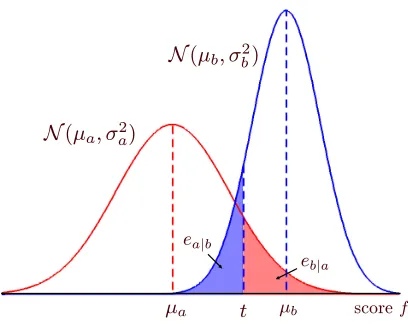
Consider for now a single score f , corresponding to a random variable, F.3 A usual way of mea-suring performance of a score when Equation (1) is used to estimate the class of the samples is equal error rate (EER), the false acceptance rate when the false rejection and false acceptance rates are equal. In speaker verification, a false acceptance (which we will call eb|a) is an impostor trial accepted by the system as the target speaker, and a false rejection (ea|b) is a true-speaker trial con-sidered an impostor trial by the system.
If we make the assumption that the conditional distribution of the scores for each class is Gaus-sian, we can obtain an explicit bound for the EER as a function of the Mahalanobis distance between the class-conditional means. Figure 1 shows how to calculate the EER for this case. We assume that the class-conditional distribution of the scores is given by
F|Y =y∼
N
(µy,σ2y), for y=a,b,where Y is the random variable corresponding to the trial’s class. We further assume, without loss of generality, that µb≥µa, so that (1) is the best way of assigning the labels for a given threshold.
Figure 1: EER calculation when the class-conditional distributions are Gaussian. The EER is equal to ea|bwhen t is chosen such that ea|b=eb|a.
With these assumptions we can compute ea|band eb|afor a certain value of the threshold t as
ea|b(t) = φ
t−µb σb
, (2)
eb|a(t) = 1−φ
t−µa σa
, (3)
whereφis the cumulative distribution function of the standard normal distribution
N
(0,1).The EER is given by eb|a(t∗)when t∗is chosen such that eb|a(t∗) =ea|b(t∗). In the appendix we prove the following upper bound on the EER:
EER=eb|a(t∗) =ea|b(t∗)≤φ(− 1 2
δµ
σ), (4)
where δµ=µb−µa, and σis any value that satisfiesσ≥(σa+σb)/2. Equality is achieved for σ= (σa+σb)/2, but this value ofσdoes not result in a nice expression later on, when we want to use it to optimize the combination performance. On the other hand,
σ=
q
(σ2
a+σ2b)/2
also satisfies the inequality and does result in a nice expression that we can later use. In the rest of the paper we will use
M
2= 2δµ2 σ2
a+σ2b
(5)
as a surrogate for the EER of the system.
M
is the Mahalanobis distance between two Gaussian distributions with distance between the meansδµ and variance(σ2a+σ2b)/2. Using (4), we get that EER≤φ(−
M
5 10 15 20 25 5
10 15 20 25
Actual EER
EER under Gaussian assumption
Upper bound Exact value
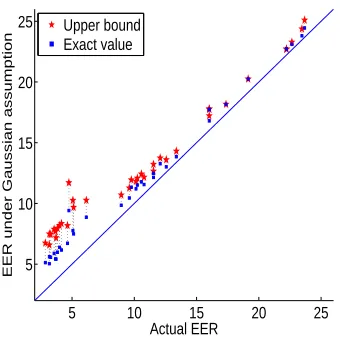
Figure 2: Actual EER for a set of 37 systems versus the upper bound and the exact value under Gaussian assumptions.
Our strategy in the remainder of the paper will be to reduce the value of the upper bound, with the hope that this will result in a reduction of the EER. Sinceφis monotonically increasing in its argument, decreasing the value of−
M
(or increasing the value ofM
) will decrease the value of the upper bound.Figure 2 shows a scatter plot of the actual EER for a set of 37 different individual systems us-ing different features or different modelus-ing techniques (some of these systems are described by Ferrer et al. (2006)) versus the upper bound on the EER under Gaussian assumption given by
φ(−δµ/q2(σ2
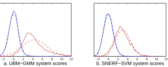
a+σ2b))and the exact value of the EER, also under Gaussian assumption, given by φ(−δµ/(σa+σb)). We can see that the upper bound is tight for high EER values. When the differ-ence between the class-conditional covariance for both classes is large (which, in our experiments, is the case for the better systems), the upper bound becomes looser. We see that the exact estimation under the Gaussian assumption performs significantly better in this case. The remainder of the error is due to the inaccuracy of the Gaussian assumption. Figure 3 shows the actual distribution of two of the systems used in this paper compared to their Gaussian approximation. Figure 3.a corresponds to one of the low EER systems that drifts away from the diagonal in Figure 2, while 3.b corresponds to a system with EER around 12%. We can clearly see that the Gaussian approximation in this case is inaccurate, which in turn explains the inaccuracy of the upper bound and the exact formula developed in this section. Interestingly, even when the Gaussian approximation is inaccurate, (4) seems to still hold. Our procedure of trying to minimize this upper bound in the hope that the actual EER will be pushed down would then still be valid.
3.2 Maximum Mahalanobis Distance Combination
−2 0 2 4 6 8 10 12
a. UBM−GMM system scores
−2 0 2 4 6 8 10 12
b. SNERF−SVM system scores
Figure 3: Distribution of scores for two individual systems compared to their Gaussian approxima-tion.
several subsystems given their individual EERs (or
M
s) and the average class-conditional covari-ance matrix for the vector of scores. To do this we further assume that the combination is performed with a linear function of the individual scores. This is not a very restrictive assumption for speaker verification since for this task we have repeatedly found that linear combination procedures perform as well (or better) than nonlinear ones (Ferrer et al., 2008a). The form of the combined scores as a function of N individual scores is thenfc= N
∑
i=1
αifi=αtf,
whereα= (α1. . .αN)t is the vector of weights and f = (f1. . .fN)t the vector of individual scores. We assume that the class-conditional distribution of the fi’s is jointly Gaussian. Hence, each of the individual scores and the combined score satisfy the assumptions made in the previous section. The class-conditional distributions of Fc, the random variable corresponding to the combined score, are given by
Fc|Y =y∼
N
(αtµy,αtΣyα), for y=a,b,where µy= (µy1. . .µyN)is the vector of means andΣy=E[(F−µy)(F−µy)t|Y =y]the covariance matrix for class y for random variable F corresponding to vector f . We can now compute
M
2 (Equation 5) for the combined score as a function of the parametersα:M
2= 2(αtµ
b−αtµa)2 αtΣ
aα+αtΣbα = α
t∆∆tα
αtΣα , (6)
where∆=µb−µaand
Σ=1/2(Σa+Σb). (7)
We wish to find the α that maximizes this expression. Define β=Σ1/2α, where Σ1/2 is a symmetric matrix square root of Σ(which can be computed from the eigendecomposition of Σ, which exists and can be chosen to be symmetric sinceΣis symmetric). Replacing this in (6), and using the Cauchy-Schwarz inequality,
M
2 = βtΣ−1/2∆∆tΣ−1/2β
βtβ =
k∆tΣ−1/2βk2
kβk2
with equality whenβ ∝ Σ−1/2∆. Hence, the optimalαis a vector in the direction ofΣ−1∆.4
Note that we have arrived at the definition of the Mahalanobis distance in multiple dimensions (∆tΣ−1∆), which is an intuitive result. We now know that the EER of the combination of the indi-vidual systems will be at mostφ(−√∆tΣ−1∆/2). If we can devise a way of increasing∆tΣ−1∆, this upper bound will decrease.
Anderson and Bahadur (1962) consider the problem of finding all the admissible linear pro-cedures for classifying into two multivariate normal distributions. They show that α= (taΣa+
tbΣb)−1∆corresponds to an admissible procedure for any taand tb(that is, no other linear procedure will have, simultaneously, strictly better eb|a and ea|b) as long as taΣa+tbΣb is positive definite. Unfortunately, the values for taand tbthat correspond to the EER have to be numerically obtained. No explicit expression is available for the general case. Since our purpose here is to obtain a simple explicit expression for the EER (as a function of the EERs of the individual systems and some other parameters) that we can use to analyze the problem, we have settled for a bound on the EER instead of using the implicit expression developed by Anderson and Bahadur.
3.3 Analysis for Combination of Two Systems
We now focus on the case N=2. In this case, we have that the optimal
M
2(∆tΣ−1∆) is given byM
2 = δ21σ22+δ22σ11−2δ1δ2σ12σ11σ22−σ212 =
M
2
1 +
M
22−2ρM
1M
21−ρ2 , (8)
whereδi is component i of vector∆, σi j is component i j of matrixΣ,
M
1=δ1/√σ11 andM
2= δ2/√σ22are the Mahalanobis distances for the individual systems, andρ=σ12/√σ11σ22. (9)
Note that ρis not the correlation between the two systems in the usual sense, since Σis not the covariance matrix of F, but the average class-conditional covariance.
Let us call the upper bound on the EER, ˆe, that is, ˆe=φ(−
M
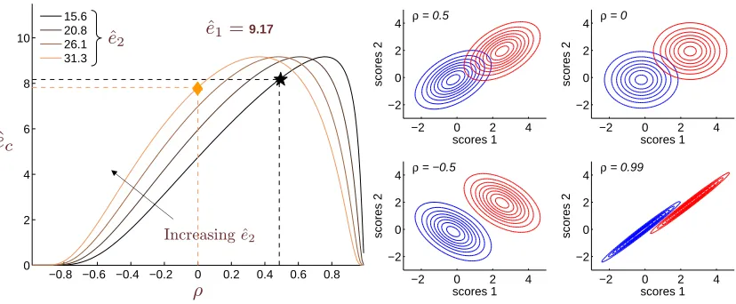
/2). Figure 4 shows some curves of ˆec, the upper bound on the performance of the combination for two systems, as a function ofρ. To create these plots we take two actual systems (the MLLR-SVM and the SNERF-SVM, as described in Section 6.2) and compute the upper bound on the EERs based on their Gaussian approximation. We also compute matrixΣand from there,ρ. This gives a single point in this graph (marked with a star). We can now varyρ, keeping ˆe1and ˆe2(the upper bound on the performance of the individual systems) fixed, to obtain a curve. We can also obtain curves for different values of ˆe2. These curves show us the relation between the performance of system 2, the value ofρbetween the two systems, and the performance of their combination. We can see that for this particular set of systems, we could degrade the second system 100% (that is, from 15.6% to 31.3%) and still get a gain in the−0.8 −0.6 −0.4 −0.2 0 0.2 0.4 0.6 0.8 0 2 4 6 8 10 15.6 20.8 26.1 31.3
Increasing ˆe2
ˆ
e2 ˆe1=9.17
ˆ
e
cρ
−2 0 2 4
−2 0 2 4 scores 1 scores 2
ρ = 0.5
−2 0 2 4
−2 0 2 4 scores 1 scores 2
ρ = 0
−2 0 2 4
−2 0 2 4 scores 1 scores 2
ρ = −0.5
−2 0 2 4
−2 0 2 4 scores 1 scores 2
ρ = 0.99
Figure 4: Left: Curves of ˆec(the upper bound on the EER of the combination) for two systems as a function ofρ, for ˆe1fixed and various values of ˆe2, where ˆeidenotes the upper bound on the EER of system i. Right: Simulated contour plots for the scores of two systems assum-ing class-conditional distributions are Gaussian with equal covariance matrix. Marginal distributions are kept fixed for all four figures, onlyρis changed. These plots correspond to four different points in the darker curve from the left plot.
performance of the combination (or at least in the upper bound) over what we get with the original pair of systems if, at the same time, we were able to decrease theρ from 0.48 to 0 (this point is denoted by a diamond in the graph).
At first sight, these curves may seem to go against intuition, since when ρ increases, after reaching a peak (occurring at the minimum of
M
1/M
2andM
2/M
1), they go down again. That is, very high values ofρresult in extremely good combination performance. Similarly, whenρturns negative, the combination performance improves, reaching zero EER forρ=−1. All these cases can be easily understood using contour plots of the scores from two systems for varying values ofρ. The right plot of Figure 4 shows four different cases. Here we keep the marginal distributions of the systems fixed and vary only ρ, which implies that the performance of the two individual systems stays fixed for the four different plots. That is, the four plots correspond to four different points in a single curve like the ones in the left plot. Furthermore, we set the covariance matrix between the two systems to be the same for both classes. In this way, the upper bound (4) is exact andρis the within-class correlation (assuming both classes have the same prior). We can see that the separation between the two classes is highly dependent on the value ofρ. The first plot shows a typical case, where ρ=0.5. The second plot shows the case of ρ=0. We can already see that the overlap between the two classes has been significantly reduced, even though the marginal distributions have not changed. The third plot shows the case of negativeρ. This implies that both systems produce errors in a negatively correlated way, which makes the combination of those two systems extremely effective at reducing the error rate. The fourth plot illustrates the case in which
covariance matrix except possibly for a scalar factor (so that the contour plots become parallel lines) and the mean vectors for both systems are different. This case corresponds to a zero value in the denominator of (8) and a nonzero at the numerator.
In practice, if we take pairs of all 37 systems plotted in Figure 2 and compute the actualρand theρat the peak (that is,ρpeak=min(
M
1/M2,M2/M1)) we find that, on average, the actualρis 0.26 to the left ofρpeak. Considering this empirical fact it seems unreasonable to try to increaseρ in order to improve the combination performance, since it would require a large increase in order to go past the peak into an area where the combination performance is better than the original. Furthermore, this would work only if the class-conditional covariance matrices were equal, which is usually not the case. Hence, in this paper, our strategy will be to try to decrease the value ofρ. Of course, we also require that the performance of each individual system stays reasonably close to its original performance, which we hope will result in a new point (in a plot like the one in the left of Figure 4) located toward the left and lower than the original point. In the next section we introduce our method for achieving this goal.4. Anticorrelation Kernel
Suppose that two separate classifiers S and B are available, where S is required to be an SVM, but B can be any classifier that produces a score for each sample. We will consider B to be a black box from which we have only the scores that it produces. As we have been assuming, the final classification decision will be made based on a combination of the outputs generated by both classifiers. Our strategy will be to train system S using information about system B in order to improve the combination performance over the one obtained when system S is designed with no knowledge of system B.
4.1 Support Vector Machines
Consider a labeled training set with m samples, T={(xj,yj)∈
R
d×{−1,+1}; j=1, ...,m}, wherexj is the feature and yj the class corresponding to sample j. The goal is to find a function f(x) =
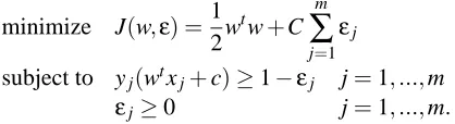
wtx+c, such that sign(f(x))is the predicted class for feature vector x. The standard (primal) SVM formulation for classification is given by Vapnik (1999):
minimize J(w,ε) =1 2w
tw+C
∑
mj=1 εj
subject to yj(wtxj+c)≥1−εj j=1, ...,m εj≥0 j=1, ...,m.
(10)
function K(xk,xl)can be easily computed. In the next section we will develop the proposed method considering an inner product kernel. The general case will be treated in Section 4.5.
The above setup corresponds to a classification problem. The regression problem can also be posed as a convex optimization problem by choosing an appropriate distance measure (Vapnik, 1999; Smola and Sch¨olkopf, 1998) with the objective function given by the sum of the square norm of the weight vector and an error term, as in the classification case. The dual of this problem again takes a form in which features appear only in inner products with other features, which again allows for the kernel trick to be used. Hence, even though the derivations in this paper will be done considering a classification problem for simplicity, the method described and the interpretations given can be equally applied to SVM regression problems.
4.2 Modified Support Vector Machines
As we saw in Section 3.3, reducing theρvalue between system S and system B could lead to an improvement in combination performance as long as the performance of the individual systems does not degrade too greatly. We propose to add a term in the SVM objective function (J(w,ε)in Equation (10) that introduces a cost for a model that results in high value ofρ. Ideally, we would like this term to be given byλρso that low values ofρare encouraged, including negative ones. Unfortunately, this term would make the new objective function nonconvex, making the optimization problem much more complex. To see this, let us derive an expression forρas a function of the SVM weights. Let S=wtX+c, where w and c are the SVM parameters. We can computeσ12=σSB (component 1,2 of Equation 7) as5
σSB = 1 2y=
∑
{a,b}
E[(B−µb,y)(S−µs,y)|Y =y] =wtK,
where we are using the notation µv,y=E[V|Y =y]for any random variable V (scalar or vectorial), and where
K = 1
2y=
∑
{a,b}
E[(B−µb,y)(X−µx,y)|Y =y]. (11)
K is simply the vector of average class-conditional covariances between each input feature and the
scores from system B. The value of vector K can be estimated from the training set T as
˜
K=1 2y=
∑
{a,b}1
my j|
∑
y j=y(bj−˜µb,y)(xj−˜µx,y), (12)
where bj is the score generated by system B for sample j, my is the number of samples in T from class y, ˜µb,y=my1 ∑j|yj=ybj, and ˜µx,y=
1
my∑j|yj=yxj.
Similarly, we can computeσ11=σSS(component 1,1 of Equation 7) as wtMw, where M is the average class-conditional covariance matrix for the feature vector X ; and σ22=σBB (component 2,2 of Equation 7) as the average class-conditional variance for the B scores that we will call v. We can now writeρ2as
ρ2= σ2SB σSSσBB
=w tKKtw
v wtMw.
This expression and its square root are nonconvex functions of w. Hence, adding the termλρto the objective function of the SVM problem would make the optimization problem nonconvex. On the other hand, the numerator ofρ2,σ2SBis a convex function of w and, using it as a regularization term results in a new problem that is equivalent to a standard SVM problem with a new kernel function. To see this, write
Jσ(w,ε) = 1 2w
tw+λ 2w
tKKtw+C
∑
i εi
= 1 2w
tAw+C
∑
i εi,
where A=I+λKKt is a symmetric positive semidefinite matrix. We can now change variables ˜
w=Bw, with B symmetric and BtB=A (i.e., B is a matrix square root of A and, since A is a
positive definite symmetric matrix, it always exists and can be chosen to be real and symmetric) and write it as
minimize Jσ(w˜,ε) =1 2w˜
tw˜+C∑ jεj
subject to yj(w˜tzj+c)≥1−εj j=1, ...,m
εj≥0 j=1, ...,m,
where
zj=B−1xj. (13)
We see that the appropriate choice of regularization term led us to a very simple new opti-mization problem. The disadvantage of this choice is that it does not directly achieve our goal of minimizingρ. For example, negative values ofρcorresponding to negative values ofσSBwill gen-erally not be encouraged by the new objective function because the maximum margin (that is, the minimum value of wtw) corresponds, in most practical cases, to positive values ofσSB. Hence, in practice, for each negative value ofσSBthe corresponding positive one will result in a smaller value of the objective function and will be preferred to the negative one. Furthermore, minimizingσSB does not imply minimization ofρ, even for positive values, since the denominator is not being taken into account. Nevertheless, we empirically find that the new optimization problem achieves its goal of reducingρ. In particular, whenλis large,σSBis pushed toward zero, forcingρto become zero.
Directly finding the matrix B−1in (13) is computationally expensive since in general the dimen-sion d of the feature vectors xi can be very large and the matrix B is a full matrix of size d×d. Nevertheless, since matrix A has a very particular structure, we can find an expression for its inverse using the matrix inversion lemma, by which A−1 =I−1+λλKtKKKt. Hence, one way of imple-menting the proposed method is to define a kernel K(xk,xl) =xtkB−tB−1xl=xtkA−1xl to be used by the SVM. This kernel satisfies the mercer conditions (i.e., it is a valid kernel) since A is a positive semidefinite matrix. Using the expression for A−1above we get
K(xk,xl) =xtkxl− λ
1+λKtKx t
kKxtlK. (14)
note that the matrix B−1is a matrix square root of A−1. Hence, we need to find a matrix that when multiplied by its transpose results in A−1=I−1+λλKtKKKt. It is easy to show that
B−1=I− α KtKKK
t
satisfies this condition whenα=1±√ 1
1+λKtK. Hence, given a certain value forλwe can find the correspondingαand transform each feature vector using (13). This means that we can implement the proposed method by transforming the input features using the following expression:
zi=xi−α
Ktxi
KtKK. (15)
In the case of speaker verification, a separate K vector is computed for each target model being trained. Hence, doing the transformation in the feature domain is inefficient, since there is not a single transformation for each feature vector xi, but one for each target model. The kernel imple-mentation might be preferable in this case. Furthermore, as we will see in Section 4.5, when the original SVM problem uses a kernel other than the inner-product one, implementing the anticorre-lation method as a kernel may be the only feasible option.
4.3 Interpretation of the Modified Problem
To give an interpretation of the new SVM problem, we first need to understand the meaning of the direction given by the vector K. The average class-conditional covariance between the scores from system B and the scores from system S is given by wtK. For a fixed value ofkwk=c, the w that
maximizes the absolute value of wtK is given by w=cK/kKk. Hence, K gives the direction for the vector w of SVM weights for which the average class-conditional covariance between the two systems is maximum. A w orthogonal to K would result in zero average class-conditional covariance between the two systems. The termkwtKk2that we have added to the objective function of the SVM problem has the effect of penalizing any w vector with a large component in the direction of K. Our goal is to find a w as orthogonal to K as possible without degrading the performance of the system so much that the overall combination starts to degrade. This balance can be achieved by tuning the parameterλ.
We can interpret the kernel given by (14) in a similar way. Whenλis small this kernel is close to the linear kernel. Whenλgrows to infinity the kernel subtracts the product of the projections of the points xkand xlinto the vector K from the linear kernel. The resulting value of the kernel will be small if xkand xlare both aligned with K. Since the SVM will make an effort to separate only points from different classes that give a high kernel value (that is, that are more “similar”), this means that we consider vectors whose directions are close to that of K to be unimportant and, consequently, we emphasize the importance of the vectors whose directions are orthogonal from that of K. This results in a more effective usage of the features, ignoring those directions that would lead to high average class-conditional covariance between the systems and taking advantage of the rest.
Finally, if we choose to implement the method as a feature transform instead of a kernel function, the resulting features have a very simple interpretation. Whenλ=∞, Equation (15) becomes zj=
xj−K tx
j
4.4 Extension for Multiple Preexisting Scores
An extension to the presented method can be considered where N previous systems are available,
B1,. . . , BN, and we wish to train S to combine well with them. A generalization of the formulas above can be derived for this setup. We rewrite the objective function as
Jσ(w,ε) = 1 2w
tw+
∑
Nk=1 λk
2w tK
kKktw+C
∑
iεi
= 1 2w
tAw+C
∑
i εi,
where now A is given by I+∑N
k=1λkKkKkt and it is still positive definite and symmetric. The same approach used above can be used here to simplify the problem to a standard SVM problem. We can still use the inversion lemma by considering matrices
K = [K1. . .KN], Λ = diag(λ1. . .λN), so that I+∑N
k=1λkKkKkt =I+KΛKt. We can then use the lemma to get A−1 =I−K(Λ−1+
KtK)−1Kt. When λ
k =∞ for all k, A−1 =I−K(KtK)−1Kt. This matrix is idempotent (and symmetric), hence B−1 =A−1. The transformed features zi for this case are then given by zi=
xi−K(KtK)−1Ktxi, which is the projection of xi on the complementary space to that spanned by vectors K1through KN.
4.5 Extension for General Kernels
The development on Section 4.2 was done using inner-product kernel SVMs as the starting point. In this section we show that the method can be implemented for any kernel function.
Consider a problem for which K0(x,y) =φ0(x)tφ0(y)has been found to perform better than the inner-product kernel. One way of implementing the anticorrelation method in this case is to simply transform the features usingφ0(x) and then treat the transformed features as the feature vectors x in Section 4.2. This is conceptually simple, but could be extremely costly computationally if the dimension ofφ0(x)is large compared to the dimension of x, or impossible if the transformationφ0 is infinite dimensional (as in the case of the Gaussian kernel). Luckily, there is a way of implement-ing the anticorrelation method without ever computimplement-ing the transform but only the kernel function between pairs of features.
In Section 4.2 we found that one way of implementing the proposed method is by the use of the
anticorrelation kernel, defined by Equation (14). In practice, vector K in that equation is computed
from data. We call this empirical value for K, ˜K (Equation 12). We can write ˜K as a linear function
of the features xj used to compute it. That is, ˜K=∑jcjxj, where the cj depend on the my’s and all the bi’s. If we now replace every x in Equation (14) byφ0(x)and K by∑jcjφ0(xj), we get
K(xk,xl) = φ0(xk)tφ0(xl)−
λ∑jcjφ0(xj)tφ0(xk)∑jcjφ0(xj)tφ0(xl) 1+λ∑j∑icjcjφ0(xi)tφ0(xj) = K0(xk,xl)−
λ∑jcjK0(xj,xk)∑jcjK0(xj,xl) 1+λ∑j∑icjcjK0(xi,xj)
The anticorrelation kernel can then be computed exclusively as a function of the original kernel
K0. The processing time is now significantly increased, though, since two sums over the samples used to obtain K are needed every time the kernel is computed (the denominator in the second term can be precomputed and reused, since it does not involve xk or xl). The extension for multiple preexisting scores follows the same steps as above. In this paper, the inner-product kernel is used for all experiments.
4.6 Other Approaches
Our goal is to obtain the best possible combination performance given the available systems. The approach presented above is one path toward this goal. Two other ways of approaching this problem are considered here.
4.6.1 FEATURE-LEVELCOMBINATION
When system B is also an SVM system and the features corresponding to the samples used for training system S are also available for system B, an SVM using the features from both systems concatenated into a single vector can be trained. The resulting SVM is in itself a combination procedure, which, ideally, should make optimal use of the features from both systems. This may not be true in practice, though, since a larger feature vector increases the complexity of the system, making it more prone to overfitting the training data. A further refinement of this approach consists of weighting the vector components, assigning weight α to the features from one of the original systems and weight 1−αto the other features. This is done by multiplying the components of the square-norm of w in the SVM objective function by the inverse of the corresponding feature weight. That is, we replacekwk2=∑iw2i with∑iw2i/βi, whereβi=αfor the features from one set and 1−α for the features from the other set. This allows us to compensate for different lengths in the original vectors or to bias the training procedure to make more use of the features from the better-performing system. Feature-level combination is usually costly and sometimes even infeasible, given the large size of the original feature vectors, and can be considered only if both systems being combined are SVM systems.
4.6.2 FEATURE+SCORE COMBINATION
Another method can be considered in which we present the scores generated by system B as input features to the SVM, along with all the features from system S. Again, a larger weight can be given to the component corresponding to the score from system B than to the features from S.
5. Experiments on Artificial Data
To test the proposed kernel on a simple task, we generated data for two classes with model
Z=C ˜Z+mY,
where ˜Z is a vector of size d where the components are generated independently with normal
applied to force the maximum variance of Z to be 1. The class-dependent mean vector is given by
mY=
(0. . .0)t if Y =a (m. . .m)t if Y =b.
We take half of the features and train a linear SVM (inner-product kernel), which serves as system B. The remaining features are used to train system S starting with an inner-product kernel. The anticorrelation kernel is implemented for varying values ofλ. We create two separate sets, one for training, with 900 examples of class a and N examples of class b, and one for testing, with 10 times more data than in the training set.
The combination is performed using a linear logistic regression model, trained on the training set with the scores from the two SVM systems, B and S, for each value of λ. Since the scores obtained on the training set are overly optimistic, we use 10-fold cross-validation on the training set to create the B and S scores used to train the combiner (Kuncheva, 2004, Section 3.2.2). The scores from cross-validation for system B are also used to estimate the vector ˜K as in (12). When
only a few samples from one of the classes are available, the estimation of ˜K can be noisy. In our
simulation we vary the number of samples available for class b, keeping the number for a fixed; hence, in order to keep the variance of the estimator stable across experiments, we use only samples from class a to estimate ˜K.
Figure 5 shows the error rates for the test data for system S, system B, and the score-level combination as a function of the value ofλ, for m=3.0, N=900 and d=250. The figure also shows results for the feature-level and the feature+score combination procedures, explained in Section 4.6. The weight αfor these two systems was tuned using 10-fold cross-validation on the training set. For these two cases and for system B, the error does not depend onλ. On the other hand, the value ofρbetween S and B decreases withλ(reaching a value close to zero). We see that, in practice,
ρis effectively reduced asλincreases, even though we useλσ2SB as regularization term instead of
λρ2. The error for system S also varies withλ. The degradation in performance is expected since we are trading off poorer performance in exchange for a lower value ofρ. The small improvement at moderate values ofλ, though, is not too surprising. If the direction K corresponded to one that is especially noisy, reducing the importance of that direction can lead to improved performance. We will see more on this in Section 6.5.
The feature-level and feature+score combination methods perform approximately equal at around 1% EER, while, forλ=0, the score-level combination has a significantly worse performance of 1.58%. Nevertheless, asλgrows, the performance of the score-level combination using the anticor-relation kernel improves significantly (from 1.58% to 0.56% whenλgoes from 0 to 104), making it the best-performing system. Overall, we see a reduction in EER of around 50%, relative to the EER of the best combined system when the anticorrelation kernel is not used.
Figure 6 shows the scatter plot of scores (on the training data) for both systems corresponding toλ=0 andλ=10000. We can see that for the large value ofλ, the within-class covariances have been largely reduced. We can also see that the separation of the two classes is better for the larger
λ, which explains the performance improvement observed in Figure 5.
Figure 7 shows the results for the score-level combination of systems B and S withλ=0 (that is, without using the proposed method), the score-level combination withλ=∞, the feature-level combination, and the feature+score combination, for several settings of the simulation parameters
10−2 100 102 104 0
1 2 3 4 5
λ
ρ
0.2 0.4 0.6 0.8 1
EER
System B EER System S EER
Score−level combination EER Feature−level combination EER Score+Feature combination EER
ρ
Figure 5: Error of individual systems and their combination, and value of the ρ coefficient as a function of λ for an artificial problem. The EER of the combination is reduced from 1.58% to 0.56% asλincreases.
−6 −4 −2 0 2 4 6
−8 −6 −4 −2 0 2 4 6
B scores
S scores for lambda = 0
−6 −4 −2 0 2 4 6
−3 −2 −1 0 1 2 3
B scores
S scores for lambda = 10000
Figure 6: Scores from system B versus scores from system S for two values ofλ.
the data ourselves according to a model, we can compute K exactly using (11) instead of (12). It can be shown that, for our setup, K = 1
2∑y={a,b}(C12C11t +C22Ct12)wB, where wB is the SVM weight vector for system B and Ci j is block i j of size d/2×d/2 of matrix C. For each set of parameters, 10 different random seeds were used to generate the data, keeping matrix C equal for all 10 experiments. Each bar shows the first quartile, the median, and the third quartile of the set of EERs obtained from the 10 simulations.
100 300 900 0.5 1 1.5 2 2.5 3 3.5 N EER
m = 3 d = 250 Feat+score
Score Feat Antic (est) Antic (real)
100 300 900
0.5 1 1.5 2 2.5 3 3.5 N EER
m = 3 d = 1000
100 300 900
4 6 8 10 12 14 16 N EER
m = 1.8 d = 250
100 300 900
4 6 8 10 12 14 16 N EER
m = 1.8 d = 1000
Figure 7: Comparison of EER on simulated data for the score-level combination of system B with
S withλ=0 (called Score in the legend), the score-level combination withλ=∞
(An-tic) using the estimated value for K (est) or the value obtained from the model (real),
the feature-level combination (Feat), and the feature+score combination (Feat+score) for several values of the simulation parameters. For each pair of m (distance between means) and d (feature vector dimension), three values of N (number of samples from class b) are explored.
plain score-level, feature+score and feature-level combinations. For m=3.0, the anticorrelation method significantly outperforms all other combination methods for both values of d and the three values of N. Gains are smaller or disappear when the task becomes harder (m=1.8).
The difference between the fourth and the fifth bars in each set is due only to the difference in the K vector used. The K is estimated using the data (Equation 12) for the fourth bar and using the model (Equation 11) for the fifth bar. We can see that when the dimension of the feature vector
6. Experiments on Speaker Verification
Speaker verification is the task of deciding whether or not a speech sample was produced by a certain target speaker. It is a binary classification task where the two classes are true-speaker and
impostor. To test the proposed method we use a standard UBM-GMM system, a cepstral supervector
SVM system, an MLLR-based system, and a prosodic system. We show results using the proposed kernel on all possible combinations involving two systems (two-way combinations) and a variety of combinations involving three and four systems (three-way and four-way combinations).
6.1 Databases and Error Measures
Experiments were conducted using data from the NIST speaker recognition evaluations (SRE) from 2005 and 2006. Each speaker verification trial consists of a test sample and a speaker model. The samples are one side of a telephone conversation with approximately 2.5 minutes of speech. We consider the 1-side training conditions in which we are given 1 conversation side to train the speaker model. This conversation corresponds to a positive example when training the SVM model for the speaker. The data used as negative examples for the SVM training and to estimate the K vectors is taken from 2003 and 2004 NIST evaluations along with some FISHER data, resulting in a total of 4355 samples. The tasks contain 26,270 trials for SRE05, and 21,343 for SRE06. In both cases around 1/10th of the trials are target trials. Trials are created by reusing the conversations from a few hundred speakers as train and test samples, sometimes as target speakers, sometimes as impostors. A total of 598 distinct models for SRE05 and 584 for SRE06 are created, some of them corresponding to different conversations from the same speaker.
The performance measures used in this section are the EER and NIST’s detection cost function (DCF). The DCF is defined as the Bayesian risk with probability of target equal to 0.01, cost of false alarm equal to 1, and cost of miss equal to 10. The DCF is affected both by the discrimination power of the system and its calibration, given by the choice of threshold that is believed to minimize it (Brummer and du Preez, 2006). In this paper, we will not explore the calibration issue, which is, in itself, a large field of study in the biometrics community. We will present results in terms of the DCF achieved when choosing the threshold that minimizes it on the test data. This measure is commonly called minimum DCF and it measures how much information the detector could have
delivered to the user, if the calibration had been perfect (Brummer and du Preez, 2006).
The EER and the DCF are two points in the receiver operating characteristic (ROC) curve of a system and they give a more complete picture of the behavior of the system for different operating points than the EER alone. Even though the theory in Section 3 was developed for EER, we will see that improvements are obtained for both performance measures.
6.2 Individual System Descriptions
6.2.1 UBM-GMM SYSTEM(G)
This is probably the most widely used paradigm for speaker verification. A Gaussian mixture model (GMM) is trained using data from many different speakers and recording conditions to create a
uni-versal background model (UBM). The target speaker models are trained by maximum a posteriori
adaptation of the background model to the training data. For a given test sample the logarithm of the ratio of the likelihoods for the target model and the background model is used as a score. The system used here is based on 13 mel frequency cepstral coefficients (MFCCs) without the zeroth-order co-efficient, and first-, second-, and third-order difference features, resulting in 52-dimensional feature vectors. The features are modeled by 2048 mixture component GMMs. Only the GMM means are adapted to the observed data, leaving variances and weights untouched. For implementation details on this system see Shriberg et al. (2005).
6.2.2 SUPERVECTOR-SVMSYSTEM(V)
This system (Campbell et al., 2006) is a variation of the UBM-GMM system, where SVMs are used to obtain scores. For each sample, the means of the UBM-GMM are adapted to the sample’s data and stacked together in a single high-dimensional feature vector. A set of held-out samples (generally the same samples used to create the UBM-GMM) is used as negative examples when training the SVM, while the target sample is used as the positive example. These features are used to train a model using support vector regression with an inner-product kernel. The signed distance to the hyperplane is then used as the output of the system. For this system we use a 512-component background model. Since the dimension of the original space is 52, the final dimension of the feature vectors is given by 512×52=26,624. Larger background models have been found to give slightly better performance but increase the computational cost of the experiments. We found 512 components to give a good balance between performance and computational cost of the system.
6.2.3 MLLR-SVM SYSTEM(M)
6.2.4 SNERF-SVM SYSTEM(S)
This system models syllable-based prosodic NERFs (nonuniform extraction region features) (Shriberg et al., 2005). Features are based on estimated F0, energy, and duration information extracted over syllables inferred via automatic syllabification based on automatic speech recognition output. Prosodic feature sequences are transformed into fixed-length vectors by a particular implementa-tion of the Fisher score (Ferrer et al., 2007). In this paper, only features modeling sequences of two syllables are used. In previous work we have found that these features by themselves yield a per-formance almost as good as using features extracted for sequences of 1, 2, and 3 syllables together. The resulting feature vector, of dimension 13,343, is first rank-normalized (as in the MLLR system) and modeled using the same procedure as for the supervector-SVM system.
6.3 Application of the Proposed Method to the Speaker Verification Problem
Most speaker verification systems that use SVMs as models consider each train or test utterance as a single sample. If necessary, as in the case of the SNERF features and many other cases presented in the literature (Ferrer et al., 2006; Brummer et al., 2007; Reynolds et al., 2005), a transform is applied to the input features prior to SVM modeling in order to convert them into a single fixed-length vector. In other cases, such as the MLLR system, the features are directly generated as a single fixed-length vector. In our experiments, since we are presenting results on the 1-side training condition from NIST evaluations, this implies that only one positive sample is available during training for each speaker model. This means that the estimation of K in (12) will be given only by impostor samples. These impostor samples are extracted from a held-out set. For each target model in the task definition we require a separate vector K. This results in significant overhead during training since each model from system B must be tested against the held-out set used to compute K. Nevertheless, this has no effect at test time. Once the vector K for each target model is computed, obtaining the score for a new test is almost as fast as for a linear kernel SVM.
6.4 Results
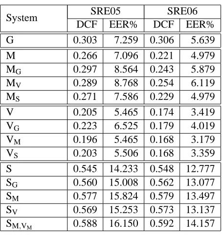
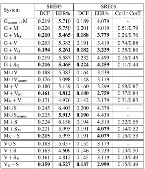
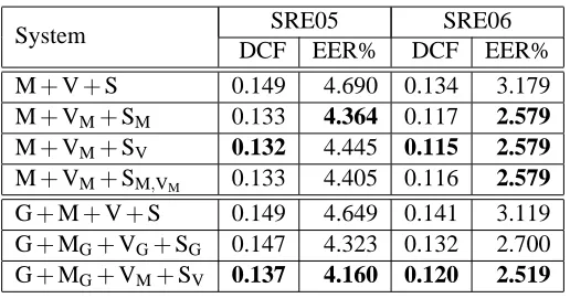
Table 1 shows the results on SRE05 and SRE06 data for the individual systems. Each system is represented by a single letter: G for the GMM-UBM, V for the Supervector-SVM, M for the MLLR-SVM, and S for the SNERF-SVM. For the SVM systems (Supervector, MLLR, and SNERFs), we show the baseline results (training the SVM with an inner product kernel) and the results obtained by training the target SVMs using the kernel in (14) with K computed using the scores corresponding to each of the other three systems. This is indicated by the use of a subindex corresponding to the system with respect to which the anticorrelation is performed. For example, MG corresponds to a system that uses the MLLR features and anticorrelation kernel with respect to the GMM-UBM system (that is, with K given by the vector of average class-conditional covariances between the MLLR features and the scores from the GMM-UBM system). A list of subindices corresponds to performing anticorrelation with respect to more than one system as described in Section 4.4. Hence, system SM,VM corresponds to system S anticorrelated with respect to systems M and VM.
System SRE05 SRE06 DCF EER% DCF EER%
G 0.303 7.259 0.306 5.639
M 0.266 7.096 0.221 4.979
MG 0.297 8.564 0.243 5.879 MV 0.289 8.768 0.254 6.119 MS 0.271 7.586 0.229 4.979
V 0.205 5.465 0.174 3.419
VG 0.223 6.525 0.179 4.019 VM 0.196 5.465 0.168 3.179 VS 0.203 5.506 0.168 3.359 S 0.545 14.233 0.548 12.777 SG 0.560 15.008 0.562 13.077 SM 0.577 15.824 0.579 13.497 SV 0.569 15.253 0.573 13.137 SM,VM 0.588 16.150 0.592 14.157
Table 1: Results for individual systems (G: GMM-UBM, V: Supervector-SVM, M: MLLR-SVM, S: SNERF-SVM) with inner product kernel and anticorrelation kernel. When the anticor-relation kernel is used, a subindex indicates the name of the system or systems with respect to which the anticorrelation is performed.
It can be seen that in most cases, using the anticorrelation kernel results in a degradation in performance in the system. A notable exception is the result for system VM(Supervector features using anticorrelation kernel with respect to the MLLR-SVM system). In this case, preventing the use of the direction given by K results in a significant gain in performance. This could happen if vector K corresponded to some noisy direction that, when ignored, allowed for other more robust directions to be used. This effect was also observed in the simulations and will be discussed in more detail in Section 6.5.