Institutions' Complementarity and Coevolution
Pak-Hung MoaHong Kong Baptist University
Abstract: I sketch a framework of theoretical and empirical models to illustrate the
interactions between government and market actors, and the resulting coevolution of related institutions. The choices and interactions of the rational actors, in addition to other stock variables, format the motivation matrix and determine the changes in economic outcomes and institutions. The changes accumulating over time reshape the institutional environment in subsequent periods. The empirical findings suggest that state variables, government policies and choices can generate virtuous or vicious spirals driving changes in institutions and the wellbeing of people for a long period of time. Understanding the mechanism is essential for building appropriate institutions and capacity to generate inclusive and sustained economic growth.
Keywords: Effects and estimations, evolution mechanism, institutional changes JEL classification: O4
1. Introduction
It is the incentive structure imbedded in the institutional/organizational structure of economies that has to be the key to unraveling the puzzle of uneven and erratic growth.
Douglas C. North
A theoretical model and the corresponding regression system are built to investigate the effects of interaction between government and market actors that drive simul-taneous evolution of trade performance and government investment across countries. More generally, the model demonstrates that the rational interactions between vested actors can explain the evolutions of economic performances, government choices and motivation structure. Given the understanding, governments can initiate economic reforms and programs that can trigger a virtuous cycle of institutional evolution favourable to sustained growth and development. This study thus relates to the literature involving motivation structure, institutions and evolution mechanism, government policy, economic growth and development.
a Department of Economics, School of Business, Hong Kong Baptist University, Kowloon Tong, Kowloon, Hong Kong. Email: [email protected]
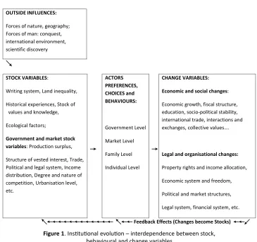
In various empirical studies, some “institutional variables” are found to have extensive effects on many and various “change variables”. For instance, Mo (2010a) found that trade per capita not only affects GDP growth rate but also the growth rates of capital and net export due to its positive effect on productivity growth; Mo (2007b) concluded that government expenditures have diverse effects on GDP growth and on changes of some supply-side and demand-side variables. As depicted by Figure 1, the accumulation of changes creates a new environment and associated motivation matrix faced by the actors in subsequent periods. The mechanism generates the “path dependent” nature of institutional evolution. Examples include the effects of geography on the choice of writing system (Mo, 2015) that in turn drive the subsequent choices of collective belief and practice, and the resulting historical evolution (Mo, 2004, 2007a).
Based on their effects on the wellbeing of communities, institutions are classified into two types: the positive and negative institutions. Positive institutions (PoINs) are institutions that induce/reduce productive/rent-seeking activities and organisations and therefore raise the long-run wellbeing of all people in a jurisdiction, and vice versa for negative institutions (NeINs). From the aspects of vested actors, we can further classify them into government institutions (GoINs) that are affected by the choices and/or outcomes of political and government actors which include voting system,
fiscal structure, laws and regulations; and market institutions (MaINs) that are largely
determined by the choices and/or outcomes of market actors which include the levels of effort allocation, productivity, capital, real GDP and trade per capita.
The complementary nature of GoINs and MaINs implies that PoINs and NeINs tend to evolve in clusters. That is, positive GoINs tend to induce positive MaINs and vice versa. Relating to the empirical studies in this paper, low international trade reduces the productivity and benefits of government investments, and therefore, discourages government investments that in turn results in low trade performance of the economy in the subsequent period. The interaction therefore results in a vicious/ virtuous spiral between trade and government investment. This can generate degrading/
upgrading spirals contributing to the decline and rise of nations.1 The models in this
study are based on the understandings and framework sketched in Figure 1. The rational government and market actors respond to the current motivation structure predetermined by the natural, international and historical environment that include geography, collective beliefs, market and socio-political organisations and other stock variables coined in the previous periods; as well as the environment created by the expectations, choices and interactions of the actors. The resulting environments format the motivation matrix that determines specific cost and benefit as well as the constraint of every choice and behaviour facing each actor. Further, the outcomes driven by the choices incrementally change the motivation structure by creating new or reshape the institutional environment which includes the structure of vested interests, power distribution, social surplus and organisations. The cumulated changes drive the evolution of the stock variables that in turn motivate the behaviours, choices and interactions of
the actors in the next period, and so on. The choice environment, motivation matrix and behaviours of the actors thus constantly evolve and changes over time. I will formulate a system of regressions in order to peek into this evolution process.
This study implies that an important developmental strategy is to institute a motivation structure that can induce both government and market actors to choose desirable actions. When the positive motivation structure is in place, complementary positive collective beliefs and practices, behaviours, power structure, organisations,
etc. will form over time under a virtuous interaction mechanism. The PoINs will thus
generate a virtuous cycle of upgrading process.2 On the other hand, a negative political
or government policy can generate a cumulative distortionary process that can result in a vicious cycle of degrading process (for instance, Olson, 1971/1982). This mechanism is demonstrated by estimations on the effects of land inequality on government investment and trade performance reported in this study, in addition to the findings of previous studies like Mo (2009b) that demonstrated the cumulative negative effects of minimum wage legislation.
In the next section, a simple model will be constructed to illustrate the interactions responsible for the long lasting effects of institutional change, and the cumulative degrading/upgrading mechanism under the rationalistic approach. The model demonstrates the virtuous/vicious interactions between government and market actors. In Section 3, the implications of the theoretical model will be empirically validated based on a well-tested data collection. And also, the role of land inequality in driving the quality of market and government institutions is also investigated. The final section concludes the findings with some related discussions.
2. The Theoretical and Empirical Models
“…the productive contribution of the society’s entrepreneurial activities varies much more because of their allocation between productive activities such as innovation and largely unproductive activities such as rent seeking or organized crime. This allocation is heavily influenced by the relative payoffs society offers to such activities.”
Baumol, 1990
Motivation structure embodies constrains, costs and benefits of different actions that govern the choice and behaviour of rational actors. This rational approach empowers us to understand and predict various market choices and outcomes. It is also used to understand historical evolution across countries (for instance, Baumol, 1990) and the choice of writing system and the characteristics of civilisations (Mo, 2015, 2016). Motivation structure is pervasively affected by “institutions” that include
formal constraints (e.g., rules, laws, constitutions), informal constraints (e.g., norms of behaviour, conventions, self-imposed codes of conduct), and their enforcement characteristics (North, 1990).
Institutional evolution can be understood according to the framework depicted
in Figure 1. Motivation structure is embedded in the stock variables that determine
the choices and effort allocation of every actor. The factors that determine the motivation structure of a nation can be classified into two types. The first is the natural environment, historical experiences and social capital such as writing system, collective values, knowledge and beliefs inherited from their ancestors in the distant past; we called these durable factors the state variables that tend to be stable and durable in a long period of time. They generate pervasive effects on behaviours, institutional characteristics and motivation matrix as exemplified in Mo (1995, 2007a, 2015, 2016). In this paper, we define institutions as the human-created environment that formats the motivation matrix of every actor in an economy. Many institutions are induced by state
Figure 1. Institutional evolution – interdependence between stock, behavioural and change variables
Sources: Modified from Hofstede, G. (1984). Culture’s consequences: International differences in work-related values, Sage Publications, Figure 1.4, p. 22; also, from Mo (2007).
OUTSIDE INFLUENCES:
Forces of nature, geography; Forces of man: conquest, international environment, scientific discovery
↘
STOCK VARIABLES:
Writing system, Land inequality,
Historical experiences, Stock of values and knowledge,
Ecological factors;
Government and market stock variables: Production surplus,
Structure of vested interest, Trade, Political and legal system, Income distribution, Degree and nature of competition, Urbanisation level, etc.
→
ACTORS PREFERENCES, CHOICES and BEHAVIOURS:
Government Level
Market Level
Family Level
Individual Level
→
CHANGE VARIABLES:
Economic and social changes:
Economic growth, fiscal structure, education, socio-political stability, international trade, interactions and exchanges, collective values….
Legal and organisational changes:
Property rights and income allocation,
Economic system and freedom,
Political and market structures,
Legal system, financial system, etc.
variables and coined by more recent choices of the actors. They include choices and interactions of the government and market actors and the resulting collective outcomes such as government expenditure structure and trade performance being studied in this paper. The data related to the changes and evolution mechanism of the induced institutions are therefore more easily observed.
The following theoretical model does not mean to be comprehensive to generalise all institutional interactions but tailor-made for understanding the interactions related to the empirical studies in this paper. The model is therefore made to be simple and concise which abstracts away many possible complications.
The choice of market actors:
At time t0, the representative market actor maximises U(M) by choosing (LV, Lr), the
respective productive activities and rent-seeking activities, with:
M = M [LV, Lr, GoIN0), subject to the constraint: LV + Lr = (1)
where M is the money income with MLV and MLr > 0; GoIN0 is the exogenous quality
of government institutions at t0; the higher/lower the GoIN0, the higher/lower the
marginal product of productive/rent-seeking activities. The second order conditions are assumed satisfied.
Optimisation implies that the higher the GoIN0, the higher the optimised
productive efforts, LV0. This raises the total factor productivity of the economy and
economic performances. At the same time, higher GoIN0 lowers Lr0.3
The choice of government actors:
Government is assumed to be short-sighted egoist targeted to maximise the net benefit from governance by choosing GoIN with:
Net Benefit = e [Y (GoIN, LV0) – survival needs] – C (GoIN) (2)
where Y is the total output with YGoIN and CGoIN > 0; e is the exogenous expropriation
rate on the social surplus that equals Y minus the survival needs; C is the cost
associated with GoIN with C’ > 0, and LV0 is the chosen productive effort of the market
actor in the last period t0. The second order conditions are assumed satisfied.
In order to capture the complementary relationship between GoIN and LV, we
assume they have the O-ring relationship such that:
Y (GoIN, LV) = GoIN*LV0 (3)
L
3 For better understanding on the relationship between GoIN, LV and economic performances, we can relate to a production function incorporated with the role of usable land (U) that depends on the quality of government inputs, such that:
where Y is the total income, V is the tools variety, X is the capital, L is the effective productive labour. GoIN, for instance, government investments and protection of private property, raises the effective supply of U directly and also, reduces transaction and production costs of market actors. It therefore changes the constraints, costs and benefits favouring productive activities and result in higher growth rate of V (Mo, 2010b). Higher productivity growth raises GDP growth as well as improvements in trade performance.
The first order condition implies: e LV0 – C’ = 0. This implies the higher the LV0, the
higher the GoIN supplied by the government when other factors are unchanged.
The model suggests that higher GoIN raises LV and this also applies to the effect
of Lv on GoIN. Through repeated interactions, the model demonstrates a possible mechanism on the dynamics of institutional evolution between the GoIN and market institutions/outcomes, such that higher GoIN results in higher/lower productive/rent seeking activities that improve market outcomes such as GDP growth rate, production surplus, tax base and trade performance, etc. that in turn promote the level of GoIN in the subsequent period. This implies:
LVt = f(GoINt); GoINt+1 = g[MaINt+1 (LVt)] (4)
with f’, g’ and MaINt+1’ > 0 with diminishing effects; t is the time, and MaINt+1 is the
quality of market institutions/outcomes at t+1 that depends on the LVt.
2.1 Empirical Models and Validation Strategy
In this empirical study, government investment (GI) and trade per capita (TRA) are
adopted to demonstrate the effects and interactions of GoIN and MaIN in the theo-retical model respectively.
Reliable input materials are essential for the success of experiments. For the estimations related to the 1970-1985 episode, all data are directly obtained from the Barro and Lee (1994) data collection. The collection is known to have generated many
consistent results in various related empirical studies.4 Adopting the well-tested data
eliminates the possible problems resulting from poor experimental material. It also allows direct comparisons between the results of this study with related studies based on a similar source of data. This strategy raises the credibility of the empirical results and generates additional values to this novel study. The Barro and Lee data collection (1994) is a panel data set starting from 1960 to 1985 and divided into five 5-year sub-periods. In the periods before 1970, we find that some essential variables have a large number of missing observations. Meaningful estimations can only start from 1970. The period 1970 to 1985 is therefore chosen for this study.
To observe the robustness of our conclusions, the results of similar estimation system for the period 1970 to 1995 are reported in the Appendix for inspection. The year ending at 1995 is intended to avoid the widespread and lingering disturbances caused by the 1997 Asian financial crisis, the 2008 financial tsunami, and the impacts of rapid advances in information technology and globalisation such that most of the observed data may not reveal the long-term relationship among various variables. All empirical results are supportive of the theoretical implications and conclusions.
The definitions and correlation coefficients of the related variables are reported in Table 1. The theoretical model is validated by empirical studies on the
inter-actions between TRA and GI for the period 1970 to 1985.5 The empirical models and
4 Among others, Mo (2000, 2001, 2003, 2009a, 2011, 2018).
Table 1 . Corr ela tion coe fficien ts and descrip tiv e st atis tics (1970-85) GIr TRAr GR TRA70 GI70 GDP70 y0 POPG POP70 PRIGHT INS TAB INS TAB70 GIr 1.00 TRAr 0.41 1.00 GR 0.57 0.63 1.00 TRA70 -0.26 0.04 -0.11 1.00 GI70 -0.20 0.11 -0.02 0.83 1.00 GDP70 -0.17 0.07 -0.04 0.88 0.90 1.00 y0 -0.28 -0.09 -0.26 0.40 0.25 0.26 1.00 POPG 0.33 -0.01 0.16 -0.39 -0.27 -0.26 -0.13 1.00 POP70 0.00 0.13 0.08 0.33 0.54 0.49 -0.01 -0.08 1.00 PRIGHT 0.35 0.02 0.07 -0.43 -0.33 -0.31 -0.40 0.67 -0.16 1.00 INS TAB -0.03 -0.12 -0.21 -0.15 -0.12 -0.11 -0.24 0.11 -0.04 0.29 1.00 INS TAB70 -0.01 -0.04 -0.11 -0.15 -0.09 -0.09 -0.18 0.10 -0.02 0.23 0.73 1.00 Mean 2.76 2.75 3.66 13,507,115 3,518,880 67,122,994 2,941 0.02 23,364 3.78 0.28 0.08 St d. De v. 1.97 1.84 2.25 31,935,267 8,948,466 216,000,000 4,080 0.01 62,273 2.03 0.40 0.16 Not es
: i)
estimations are further extended to investigate the role of an important state variable, land inequality, in driving the coevolution of the TRA and GI following the reasoning depicted in Figure 1. For inspecting the robustness of the findings and conclusions, similar estimations covering the period 1970-1995 are conducted which are reported in the Appendixes.
The system of empirical models to validate the theoretical implications related to the change in GI is formulated as follows:
(a) The relationship between stock and change: GI85 = GI70 (1 + r)15; r is the
growth rate of GI, and
GIr = GI85/GI70 = (1 + r)15 (5)
(b) Other factors unchanged, higher TRA70 correlates with higher productivity of the market sector which induces higher GIr or equivalently, higher GI85 in the subsequent period. The model is specified as follows:
GIr = a1 + a2TRA70 + a3Y70 + a4y70 + a5GR + a6Z1 + e1; with a2, a5 > 0 (6)
(c) Higher TRA70 and GI70 also raise the growth rate of real GDP (GR):6
GR = b1 + b2TRA70 + b3GI70 + b4Y70 + b5y70 + b6Z2 + e2; with b2 and b3 > 0 (7)
Substitute (7) into (6), we have the reduced form of (6):
GIr = a1 + a2TRA70 + a3Y70 + a4y70 + a5(b1 + b2TRA70 + b3GI70 +
b4Y70 + b5y70 + b6Z2 + e2) + a6Z1 + e1 (8)
where Z1, Z2 are other control variables and e1, e2 are the error terms.
(d) Since TRA70 is predetermined in the estimation system, the effects of TRA70 on the dependent change variables can be consistently estimated. Based on equation (8), the total effect of TRA70 (T) on GIr, can be decomposed as follows:
T = a2 + a5 b2 (9)
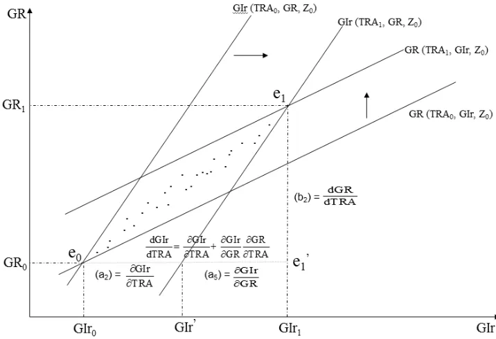
The estimation structure based on Equation (9) can be understood by the illus-tration of the coevolution process explained in Figure 2 which is equivalent to the
decomposition of the total effect of TRA on the GIr, as follows:7
(10)
6 The findings are documented in Mo (2010a and 2007b).
7 As illustrated in Figure 2, the regression system estimates the coevolving values of GIr and GR moving from e0 to e1 driven by TRA. The estimates allow us to do the decomposition exercise according to equation (9) or equivalently, (10). Since we are not estimating the coefficients related to the structural equation of GIr or GR but the coevolving path of GR and GIr driven by the stock variable, the estimator of regression (6) related to the coevolving variable does not suffer from the bias caused by simultaneity. As will be shown later, the remarkable fitness of the estimated and calculated effects in the estimations supports the validity of the theoretical and empirical models.
dGIr dTRA
GIr TRA
GIr GR
dGR dTRA = ∂
∂ +
In the estimation system, the initial trade performance (TRA70) is assumed to be the given stock variable that drives the change variables in the subsequent periods. Higher TRA70 is correlated with productive activities in the market sector which raises the return of government investment. The better MaIN captured by TRA70 thus induces higher GIr that cumulatively results in higher stock of GI over time. In the process, the higher growth rate of real GDP (GR) also raises the GIr through its positive effect
on government revenue constraint.8 Therefore, TRA70 raises GIr directly through the
motivation channel on government actors and also indirectly through the higher GR in the coevolution process. The total effect of TRA70 on GIr can be calculated according to equation (9) which should be equal to the reduced form estimation when GR is not included in estimation (6). A similar regression system can be used to investigate the effect of GI70 on the TRAr in the subsequent period.
3. Empirical Estimations and Validations
Most stock variables related to government and market institutions tend to be con-stantly evolving, interacting with and complementary to each other and also, are likely to be driven by some fundamental causes like geography, writing system and collective
Figure 2. Coevolution process of GIr and GR driven by TRA
beliefs (for instance, Mo, 2015, 2016, 2007a). They tend to be highly correlated. However, based on the reasoning and framework depicted in Figure 1, the choices and behaviours of the actors that drive the subsequent direction of evolution and changes are driven by the initial motivation matrix that is formatted by the predetermined stock variables. The stock variables GI70 and TRA70 are therefore largely exogenous to the
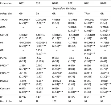
Table 2a. Coevolution between trade, government investment and growth (1970-85)
Estimation B1T B1P B1GR B2T B2P B2GR
Dependent Variables
Indep. Var. GIr GIr GR TRAr TRAr GR
TRA70 0.000387 0.000208 4.01N6 -3.37N6 -0.00012 4.01N4
(2.21)** (2.24)** (1.57) (0.047) (2.32)** (1.56)
GI70 – – – 3.84N8 2.37N8 3.72N8
(2.80)*** (2.03)** (1.99)**
GDP70 1.06N9 2.48N10 1.84N11 -6.58N10 -7.39N10 5.03N12
(2.2)** (0.87) (2.19)** (1.20) (1.84)* (0.59)
y0 -0.000356 -0.000149 -4.65N6 -1.74N5 0.000143 -4.76N6
(2.23)*** (1.91)*** (2.59)** (0.305) (2.98)*** (2.48)**
GR – 0.451 – – 0.419 –
(6.10)*** (4.69)***
POPG 4.830 -2.62 0.183 -38.5 -51.0 0.168
(0.24) (0.139) (0.54) (1.77)* (2.99)*** (0.48)
PRIGHT 1.384 0.790 0.0143 0.479 0.056 0.0131
(2.71)*** (1.98)*** (1.96)** (0.81) (0.135) (1.78)*
PRIGHT2 -0.150 -0.067 -0.00200 -0.0509 0.0113 -0.0018
(2.27)** (1.27) (2.44)** (0.74) (0.225) (2.20)**
INSTAB -1.075 -0.187 -0.0223 -0.612 0.141 -0.020
(2.87)*** (0.65) (4.84)*** (2.65) (0.56) (4.52)***
Constant 0.973 -0.375 0.029 2.12 0.845 0.030
(2.87)*** (0.66) (3.51)*** (3.84)*** (1.36) (3.59)***
R2 0.266 0.47 0.29 0.125 0.50 0.25
No. of obs. 98 98 102 97 97 98
change variables in 1970-85 and the models can therefore be consistently estimated.9
As shown in Table 2a, GI70 and TRA70 are highly correlated, however, they have the expected opposite partial effects on the change variables TRAr and GIr as shown in regressions B2T and B2P.
The empirical findings suggest that the stock variables GI70 and TRA70 drive the change variables of each other as well as GR. As expected, other factors unchanged, higher initial GI result in higher TRA and higher initial TRA raises GI over time while both of them promote economic growth of the subsequent period. Moreover, the GR coevolves with GIr and TRAr. They validate the theoretical implications that government choices, or the quality of government institutions in general, coevolves with the choices and/or outcome of market actors. This novel estimation system demonstrates the possibility of peeking into the independent motivation effect of the stock variables like TRA70 and GI70 on the choices of the respective actors when the coevolving economic growth effect is controlled. The add-up estimates also provide additional robustness check on the model specifications. In the next section, I will inspect the role of an important durable stock variable, land distribution inequality, in driving the quality of coevolving MaINs and GoINs exemplified by TRA and GI.
3.1 The Effects of Land Inequality on the Induced Variables
There is a common perception that countries with successful land reform and reduced inequality in land ownership should have higher growth than countries with no land reform. For instance, relative to the Asian countries, Latin American countries did not
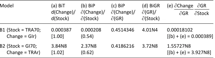
Table 2b. Coevolution between trade, government investment and growth (1970-85)
Model (a) BiT (b) BiP (c) BiP (d) BiGR (e)
d(Change)/ ∂(Change)/ ∂(Change)/ ∂(GR)/
d(Stock) ∂(Stock) ∂(GR) ∂(Stock)
B1 (Stock = TRA70; 0.000387 0.000208 0.4514346 4.01N4 0.00018102
Change = GIr) [1.00] (0.54) [(b) + (e) = 0.000389]
B2 (Stock = GI70; 3.84N8 2.37N8 0.4186216 3.72N8 1.55727N8
Change = TRAr) [1.02] (0.62) [(b) + (e) = 3.927N8]
Notes: i) (a) is the estimated total effect. (b) is the partial effect with GR included in the regressions. ii) [(b) + (e)] is the calculated total effect. The respective value in […] in column (a) is equal to [(b)+(e)] divided by (a). iii) The respective value in (…) in column (b) is equal to (b) divided by (a) which indicates the direct effect of the stock variable on the change variable after the coevolving variable GR is controlled.
∂ ∂
∂ ∂ Change
GR GR Stock
9 For observing the robustness of our conclusions, similar exercises with the data based on the period
have land reform and therefore have lower economic growth (Adelman, 1978; Alesina & Rodrik, 1994). Besides the possible channels discussed in Todaro and Smith (2011), Mo (2003) concludes that land inequality reduces GDP growth through reducing productivity growth, human capital, socio-political stability and private investment. In addition, land inequality is commonly observed to persist in a long period of time
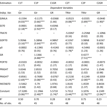
Table 3a. Land inequality on the coevolution of GI, trade and growth (1970-85)
Estimation C1T C1P C1GR C2T C2P C2GR
Dependent Variables
Indep. Var. GIr GIr GR TRAr TRAr GR
GINILA -0.1594 -0.1175 -0.0368 -0.0523 -0.0335 -0.0440
(4.03)*** (3.66)*** (1.66) (4.08)*** (3.89)*** (1.90)*
GI70 -0.0001 -0.0001 4.65N6 – – –
(2.18)** (2.92)*** (0.17)
TRA70 – – – -5.03N7 -3.25N8 -1.10N6
(0.16) (0.02) (0.20)
GDP70 5.95N6 5.38N6 4.98N7 4.51N7 3.98N8 9.61N7
(3.16)*** (3.64)*** (0.47) (0.77) (0.10) (0.90)
y0 -0.0002 -6.13N5 -9.41N5 -0.0001 -4.54N5 -0.0001
(0.76) (0.35) (0.76) (1.78)* (1.23) (1.26)
GR – 1.1366 – – 0.4277 –
(4.88)*** (7.51)***
POP70 -0.0103 -0.0032 -0.0063 -0.0032 -0.0001 -0.0073
(1.17) (0.45) (1.27) (1.17) (0.06) (1.47)
PRIGHT 3.6546 2.8533 0.7050 1.0080 0.4714 1.2546
(1.53) (1.52) (0.53) (1.42) (1.02) (0.98)
PRIGHT2 -0.8561 -0.7690 -0.0767 -0.2130 -0.1249 -0.2059
(2.69)*** (3.08)*** (0.43) (2.24)** (2.00)** (1.20)
INSTAB70 -3.5462 -5.79 1.9741 1.8145 1.4539 0.8434
(-0.68) (1.42) (0.68) (1.10) (1.37) (0.28)
Constant 17.5285 11.1966 5.5710 5.7312 3.1076 6.1349
(3.06)*** (2.40)** (1.74)* (3.44)*** (2.76)*** (2.04)**
R2 0.50 0.70 0.28 0.39 0.75 0.23
No. of obs. 45 45 45 48 48 48
(for instance, Jazairy, Alamgir, & Panuccio, 1992, Table 10). In our framework, this durable stock variable is likely to have widespread and persistent effects on the coevolution of GoINs, MaINs and other socio-political variables. To investigate this possibility, we estimate the effects of land inequality on the coevolution of trade, government investment and GDP growth. The estimations are reported in Table 3a and the decomposition results are reported in Table 3b. All results are as expected with remarkable robustness. The estimations conclude that land inequality has significant negative effects on the coevolution of GIr, TRAr and GR. The findings, in addition to Mo (2003), further confirm the “redistribution before growth” hypothesis of Adelman (1978). They suggest that equitable land rent allocation can trigger a virtuous cycle of institutional evolution favourable to sustained growth and development.
4. Conclusion and Discussion
“The organizations that come into existence will reflect the opportunities provided by the institutional matrix. That is, if the institutional framework rewards piracy then piratical organizations will come into existence; and if the institutional framework rewards productive activities then organizations—firms— will come into existence to engage in productive activities.”
North, 1994
As noted in Krueger (1974), Murphy, Shleifer and Vishny (1991), Tullock (1967), among others, in many countries talented people do not become entrepreneurs, but join the government, army, organised religion and other rent-seeking activities because these sectors offer the highest rewards. Landes (1969) suggested that the differential allocation of talent is one of the reasons why England had the Industrial Revolution in the eighteenth century but France did not. Baumol (1990) further suggested that the decline and rise of nations such as ancient Rome, early China, the Middle Ages and Renaissance are driven by the relative payoffs that society offers to productive/ innovative activities or destructive activities like rent-seeking and organised crimes. Increasing consensus has been reached that motivation structure embodied in institutions are the most important factor determining the long-term performance of
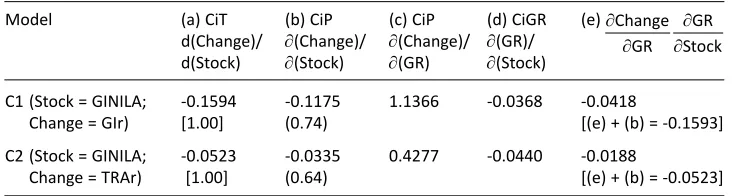
Table 3b. Land inequality on the coevolution of GI, trade and growth (1970-85)
Model (a) CiT (b) CiP (c) CiP (d) CiGR (e)
d(Change)/ ∂(Change)/ ∂(Change)/ ∂(GR)/
d(Stock) ∂(Stock) ∂(GR) ∂(Stock)
C1 (Stock = GINILA; -0.1594 -0.1175 1.1366 -0.0368 -0.0418
Change = GIr) [1.00] (0.74) [(e) + (b) = -0.1593]
C2 (Stock = GINILA; -0.0523 -0.0335 0.4277 -0.0440 -0.0188
Change = TRAr) [1.00] (0.64) [(e) + (b) = -0.0523]
Notes: Please refer to the notes in Table 2b.
∂ ∂
∂ ∂ Change
an economy (see among many others, Hoff & Stiglitz, 2001; Rodrik, Subramaniam, & Trebbi, 2004). Moreover, their effects can be felt after hundreds of years (Acemoglu, Johnson, & Robinson, 2001). In practice, almost all human-created environments that include political and market systems, government policies, organisations, religions, collective values, etc. are vaguely called “institutions” in the diverse and widespread range of literature (Williamson, 2000).
In this study, we define institutions as the human-made motivation matrix that governs the constraints, choices and behaviours of every actor who is constantly making rational decisions. The institutional variables, their role on the choices of the actors and their subsequent effects on the change variables are sketched in Figure 1. Under this definition, we build simple theoretical and empirical models to exemplify the determinants of the institutional quality and its evolution mechanism. The theoretical implications from the model are supported by real world observations about the coevolution mechanism between economic growth, government investment and trade performance. All of them are significantly affected by land inequality, an important durable stock variable, and its effects are remarkably durable as demonstrated by the estimations based on the sample period 1970-1995 as reported in Appendix Table 2a. The rational interactions between government and market actors generating the vicious/virtuous spirals of “institutional changes” can explain the lingering divergence in the quality of institution clusters across nations which can last for centuries. The interactive spiral implies that a historical accident or unintended change of government policies can cause widespread and long-lasting effects on the quality of institutions over time. This research demonstrates that the initial quality of MaINs and GoINs not only determines the short-term growth performance, but also generates spirals that drive the institutional upgrading/degrading process that reshapes the associated motivation matrix over time. All public policies and institutional choices have to take this possibility into account.
and lagged economies. We have to look into specific stock variables responsible for the causes of persistent diverging performances across countries and seek appropriate rectifications.
References
Acemoglu, D., Johnson, S., & Robinson, J.A. (2001). The colonial origins of comparative develop-ment: An empirical investigation. The American Economic Review, 91(5), 1369-1401.
Adelman, I. (1978). Redistribution before growth: A strategy for developing countries (Inaugural Lectural for the Cleveringa Chair). The Hague: Leiden University.
Alesina, A., & Rodrik, D. (1994). Distributive politics and economic growth. The Quarterly Journal
of Economics, 109(2), 465-490. doi: 10.2307/2118470
Barro R., & Lee, J.W. (1994). Data set for a panel of 138 countries. Retrieved from www.nber.org/ pub/barro.lee.
Baumol, William (1990) Entrepreneurship: Productive, unproductive, and destructive. The Journal
of Political Economy, 98(5), 893-921. https://doi.org/10.1086/261712
Hoff, K., & Stiglitz, J.E. (2001). Modern economic theory and development. In G. Meier & J.E. Stiglitz (Eds.), Frontiers of development economics: The future in perspective (pp. 389-459). New York: Oxford University Press.
Hofstede, G. (1984). Culture’s consequences: International differences in work-related values. Newbury Park, CA: Sage Publications.
Jazairy, I., Alamgir, M., & Panuccio, T. (1992). The state of world rural poverty: An inquiry into its
causes and consequences. New York, NY: New York University Press for International Fund for
Agricultural Development.
Krueger, A. (1974). The political economy of the rent-seeking society. The American Economic
Review, 64(3), 291-303.
Landes, D.S. (1969). The unbound prometheus: Technological change and industrial development
in western Europe from 1750 to the present. Cambridge, UK: Cambridge University Press.
Mo, P.H. (1995). Effective competition and economic development of imperial China. Kyklos, 48(1), 87-103. https://doi.org/10.1111/j.1467-6435.1995.tb02316.x
Mo, P.H. (2000). Income inequality and economic growth. Kyklos, 53(3), 293-315. https://doi. org/10.1111/1467-6435.00122
Mo, P.H. (2001). Corruption and economic growth. Journal of Comparative Economics, 29(1), 66-79. doi: 10.1006/jcec.2000.1703
Mo, P.H. (2003). Land distribution inequality and economic growth. Pacific Economic Review, 8(2), 171-181. https://doi.org/10.1111/j.1468-0106.2003.00218.x
Mo, P.H. (2004). Lessons from the history of imperial China. In P. Bernholz & R. Vaubel (Eds.),
Political competition, innovation and growth in the history of Asian civilization (pp. 57-87).
Cheltenham, UK: Edward Elgar.
Mo, P.H. (2007a). The nature of Chinese collective values: Formation and evolution. International
Journal of Chinese Culture and Management, 1(1), 108-125. https://doi.org/10.1504/
IJCCM.2007.016171
Mo, P.H. (2007b). Government expenditures and economic growth: The supply and demand sides.
Fiscal Studies, 28(4), 497-522. https://doi.org/10.1111/j.1475-5890.2007.00065.x
Mo, P.H. (2009a). Income distribution polarization and economic growth. Indian Economic Review, 44(1), 107-123.
Mo, P.H. (2010a). Trade intensity, net export and economic growth. Review of Development
Economics, 14(3), 563-576. https://doi.org/10.1111/j.1467-9361.2010.00573.x
Mo, P.H. (2010b). Institutions, tools variety and channels to sustained economic growth. Paper presented at the Seventh Annual Conference, Asia-Pacific Economic Association, APEA 2011, Busan University, South Korea.
Mo, P.H. (2011). Measures of income inequality and economic growth. Journal of Income Distribution, 20(3-4), 24-42.
Mo, P.H. (2015). Geography, writing system and history of ancient civilizations. Man and the
Economy, 2(1), 25-43. https://doi.org/10.1515/me-2014-0015
Mo, P.H. (2016). The nature of western and Islamic civilizations: Formation, evolution and clashes. Paper presented at: i) The Twelfth Annul Conference of the Asia-Pacific Economic Association held in Kolkata, India, 13-15 July 2016. ii) The 9th Biennial Conference of the Hong Kong Economic Association, The University of Hong Kong, 12-13 December, 2016.
Mo, P.H. (2018). Prosperity or stagnation: The role of government expenditures. Singapore
Economic Review (online), 1-24. https://doi.org/10.1142/S0217590817500242
Murphy, K.M., Shleifer, A., & Vishny, R.W. (1991). The allocation of talent: Implications for growth.
The Quarterly Journal of Economics, 106(2), 503-530. doi: 10.2307/2937945
North, D.C. (1981). Structure and change in economic history. New York, NY: W.W. Norton & Co. North, D.C. (1990). Institutions, institutional change and economic performance. Cambridge, UK:
Cambridge University Press.
North, D.C. (1994). Economic performance through time. The American Economic Review, 84(3), 359-368.
Olson, M. (1971/1982). The rise and decline of nations: Economic growth, stagflation, and social
rigidities. New Haven, CT: Yale University Press.
Pierson, Paul (2000). Increasing returns, path dependence, and the study of politics. The
American Political Science Review, 94(2), 251-267. https://doi.org/10.2307/2586011
Rodrik, D., Subramanian, A., & Trebbi, F. (2004). Institution rule: The primacy of institutions over geography and integration in economic development. Journal of Economic Growth, 9(2), 131-165. https://doi.org/10.1023/B:JOEG.0000031425.72248.85
Taylor, C.L., & Hudson, M.C. (1972). World handbook of political and social indicators (2nd ed.). New Haven, CT: Yale University Press.
Todaro, M.P., & Smith, S.C. (2011). Economic Development (11th ed.), (Chapter 9: Agricultural Transformation and Rural Development). Harlow, Essex: Pearson.
Tullock, G. (1967). The welfare costs of tariffs, monopolies, and theft. Western Economic Journal, 5(3), 224-232.
Williamson, O. (2000). The new institutional economics: Taking stock, looking ahead. Journal of
Appendixes
Appendix Table 1a. Coevolution between trade, government investment and growth (1970-95)
Estimation AB1T AB1P AB.GR AB2T AB2P
Indep. Var. GIr GIr GR TRAr TRAr
TRA70 0.0006 0.0003 0.0001 0.0001 6.44N6
(1.68)* (0.86) (1.60) (1.02) (0.08)
GI70 -4.98N5 -0.0001 2.50N5 6.30N5 4.52N5
(-0.84) (-2.51)*** (1.89)* (4.00)*** (3.48)***
GDP70 5.14N6 6.25N6 -3.98N7 -1.72N6 -1.43N6
(1.48) (2.28)** (-0.51) (-1.85)* (-1.91)*
y0 -0.0006 -0.0002 -0.0002 -0.0001 -8.16N6
(-1.91)* (-0.67) (-2.19)** (-1.40) (-0.11)
GR – 2.7734 – – 0.7111
(7.43)*** (6.96)***
POP70 -1.5201 -3.0462 0.5503 -0.5432 -0.9345
(-0.97) (-2.44)** (1.57) (-1.30) (-2.73)***
PRIGHT 8.0558 4.3509 1.3359 2.4874 1.5375
(2.42)** (1.63) (1.79)* (2.79)*** (2.10)**
PRIGHT2 -1.2330 -0.4972 -0.2653 -0.3692 -0.1805
(-2.94)*** (-1.44) (-2.83)*** (-3.29)*** (-1.91)*
INSTAB70 -7.0000 -8.3441 0.4846 -0.3313 -0.6759
(-1.00) (-1.50) (0.31) (-0.18) (-0.44)
Constant 8.1517 1.3633 2.4477 1.3420 -0.3984
(1.60) (0.33) (2.15)** (0.99) (-0.35)
R2 0.18 0.50 0.24 0.28 0.53
No. of obs. 98 98 98 98 98
Notes: i) Please refer to the notes in Table 2a. ii) The data related to 1995 is sourced from Penn World Table. iii) For providing additional observations on the robustness of our conclusions, the INSTAB in Table 2a is re-placed by INSTAB70, the initial socio-stability level. Also, TRA70 and GI70 are included in all regressions.
Appendix Table 1b. Coevolution between trade, government investment and growth (1970-95)
Model (a) ABiT (b) ABiP (c) ABiP (d) AB.GR (e)
d(Change)/ ∂(Change)/ ∂(Change)/ ∂(GR)/
d(Stock) ∂(Stock) ∂(GR) ∂(Stock)
AB1 (Stock = TRA70; 0.0006 0.0003 2.7734 0.0001 0.0003
Change = GIr) [1.00] (0.5) [(e) + (b) = 0.0006]
AB2 (Stock = GI70; 6.30N5 4.52N5 0.7111 2.50N5 1.78N5
Change = TRAr) [1.00] (0.72) [(e) + (b) = 6.30N5]
Notes: i) Please refer to the notes to Table 2a. ii) The coefficients of TRA70 in model AB1P are not statistically significant. As discussed in the notes to Table 2a, they can be caused by the collinearity problem or the effect is relatively small. We consider the estimates are valid and use them in the decomposition exercise according to equation (9). The proximity of the estimated and calculated effects supports our treatment.
∂ ∂
∂ ∂ Change
Appendix Table 2a. Land inequality on the coevolution of GI, trade and growth (1970-95)
Estimation AC1T AC1P AC1GR AC2T AC2P AC2GR
Dependent variables
Indep. var. GIr GIr GR TRAr TRAr GR
GINILA -0.4538 -0.2692 -0.0397 -0.1237 -0.0764 -0.0451
(-4.21)*** (-3.54)*** (-2.26)** (-4.11)*** (-2.97)*** (-2.53)**
GI70 -0.0002 -0.0002 5.62N6 – – –
(-1.40) (-2.42)** (0.26)
TRA70 – – – -5.19N5 -9.06N5 3.70N5
(-0.21) (-0.45) (0.25)
GDP70 1.20N5 9.47N6 5.45N7 9.62N7 1.21N7 8.03N7
(2.34)** (2.78)*** (0.65) (1.02) (0.16) (1.43)
y0 -0.0010 -0.0002 -0.0002 -0.0002 -1.40N5 -0.0002
(-1.70)* (-0.44) (-1.84)* (-1.18) (-0.09) (-1.78)*
GR – 4.6545 – – 1.0464 –
(6.89)*** (4.90)***
POP70 -0.0353 -0.0131 -0.0048 -0.0095 -0.0047 -0.0046
(-1.48) (-0.82) (-1.22) (-1.52) (-0.92) (-1.24)
PRIGHT 13.1466 7.2580 1.2651 3.8400 2.3417 1.4318
(2.02)** (1.66) (1.19) (2.39)** (1.79)* (1.50)
PRIGHT2 -2.7514 -1.5542 -0.2572 -0.7636 -0.4501 -0.2996
(-3.17)*** (-2.60)*** (-1.82)* (-3.52)*** (-2.45)** (-2.32)**
INSTAB70 -0.4698 -11.1107 2.2862 1.6053 -0.8969 2.3913
(-0.03) (-1.18) (0.99) (0.42) (-0.29) (1.06)
Constant 42.6665 11.4231 6.7125 10.7226 3.3891 7.0084
(2.74)*** (1.02) (2.64)*** (2.83)*** (1.01) (3.11)***
R2 0.45 0.77 0.36 0.45 0.66 0.38
No. of obs. 45 45 45 48 48 48
Note: Please refer to Table 3a and Appendix Table 1a.
Appendix Table 2b. Land inequality on the coevolution of GI, trade and growth (1970-95)
Model (a) ACiT (b) ACiP (c) ACiP (d) ACiGR (e)
d(Change)/ ∂(Change)/ ∂(Change)/ ∂(GR)/
d(Stock) ∂(Stock) ∂(GR) ∂(Stock)
B1 (Stock = GINILA; -0.4538 -0.2692 4.6545 -0.0397 -0.1848
Change = GIr) [1.00] (0.59) [(b) + (e) = -0.4540]
B2 (Stock = GINILA; -0.1237 -0.0764 1.0464 -0.0451 -0.0472
Change = TRAr) [1.00] (0.62) [(b) + (e) = -0.1236]
Note: Please refer to Table 3b.
∂ ∂
∂ ∂ Change