Subspace Learning with Partial Information
Alon Gonen [email protected]
School of Computer Science and Engineering The Hebrew University
Jerusalem, Israel
Dan Rosenbaum [email protected]
School of Computer Science and Engineering The Hebrew University
Jerusalem, Israel
Yonina C. Eldar [email protected]
Department of Electrical Engineering Technion, Israel Institute of Technology Haifa, Israel
Shai Shalev-Shwartz [email protected]
School of Computer Science and Engineering The Hebrew University
Jerusalem, Israel
Editor:Kevin Murphy
Abstract
The goal of subspace learning is to find ak-dimensional subspace ofRd, such that the expected squared distance between instance vectors and the subspace is as small as possible. In this paper we study subspace learning in apartial informationsetting, in which the learner can only observe r ≤dattributes from each instance vector. We propose several efficient algorithms for this task, and analyze their sample complexity.
Keywords: principal components analysis, budgeted learning, statistical learning, learning with partial information, learning theory
1. Introduction
attributes are missing, while in the second one a learner may actively choose which attributes to observe.
The subspace learning problem is formally defined as follows. Let X be a subset of the Eu-clidean unit ball inRd, and letP be some unknown distribution overX. Our goal is to find a rank-k projection matrixΠ∈Rd×dsuch that the expected squared distance,
Ex∼P[kx−Πxk22], is as small
as possible.
When X is a finite set and P is the uniform distribution over X, the optimal solution to the subspace learning problem is given by the Principal Component Analysis (PCA) algorithm, which returns the projection matrix that corresponds to thek leading eigenvectors of the matrix
1
|X | P
x∈Xxx>. In the more general stochastic optimization setting of subspace learning,X is not
restricted to be a finite set,P is an arbitrary distribution overX, and the information given to the learner has the form of an i.i.d. training sequence(x1, . . . , xm)∼Pm.
In the usual full information setting of subspace learning, the learner has access to all attributes of the sampled vectors. In this paper, we consider subspace learning in a partial information setting, in which only a subset of indices from each vector can be observed. Inspired by the two applications presented above, we study two variants of this problem, which will be named thepassivesetting, and theactivesetting, respectively. In the passive setting, we assume that each attribute is observed with probabilityp = r/d(r ≤ d). Therefore, the expected number of observed attributes from each vector isr. In the active setting, the learner can choose (possibly at random)r attributes to be revealed. The sample complexity of a subspace learning algorithm is defined as the number of samples that are needed by the algorithm in order to find a projection matrixΠ with expected squared distance, Ex∼P[kx−Πxk22], of at mostmore than the optimal expected squared distance.
The sample complexity for each of the models is defined as the minimal sample complexity attained by any algorithm. In this paper we propose efficient algorithms for both settings and analyze their sample complexity. We also provide several lower bounds on the sample complexity that can be attained by any algorithm.
1.1 Our Contribution
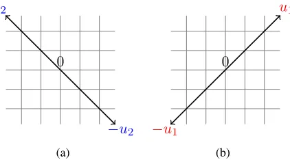
Our first observation is that subspace learning (in both the passive and active models) usingr = 1
attributes is impossible. Consider the task of learning a1-dimensional subspace (a line) inR2 (see Figure 1). Letu1 = (α, α), u2 = (−α, α). Denote byP1the uniform distribution over{u1,−u1},
and byP2 be the uniform distribution over {u2,−u2}. Suppose that the actual distribution P is
chosen uniformly at random from{P1, P2}. The task of subspace learning in this case amounts to
distinguishing betweenP1 andP2. However, since each single coordinate is distributed uniformly
over{−α, α}, the learner does not obtain any information from a single observation, and hence cannot identify the right subspace.
For the case2 ≤ r ≤ dwe propose two efficient algorithms, named Partially Observed PCA (Section 2.1) and Matrix Bandit Exponentiated Gradient (Section 3.1), which are designed for the passive and active models, respectively.
u2
−u2
0
(a)
u1
−u1
0
(b)
Figure 1: Impossibility of subspace learning usingr = 1observed attributes. The distribution of the observed attribute is identical for (a) and for (b), therefore they are indistinguishable.
the matrix m−1Pm
i=1xix>i (whose expected value is C). Similarly, the POPCA algorithm uses the random observations in order to construct an estimateCˆ ofC, and approximatesΠ? using the projection matrix onto thekleading eigenvectors ofCˆ. We analyze the sample complexity of this algorithm, showing (see Corollary 3) that it is bounded from above by(d/r)2k2.
In the full information setting, the sample complexity is known to be O(k/2) (This bounds coincides with our bound whenr = d). Hence, the (multiplicative) price of partial information, that is, how many more examples we need in order to compensate for the lack of full information on each individual example, isO((d/r)2). It is interesting to understand whether a lower price can be achieved. In Theorem 4 we prove that the sample complexity of every algorithm in the passive model isΩ (d/r)2k2
. The optimality of POPCA in the passive mode is thus established. Another appealing property of POPCA is that, in terms of computational complexity, the challenge of partial information does not incur any additional cost; While the sample complexity grows asrdecreases, the runtime per iteration decreases by the same order.
Next, we investigate the active model and ask whether the price of partial information can be reduced due to the ability of the learner to actively choose the observed attributes. Intuitively, one may hope that the learning process would reveal some useful information that can be utilized while choosing which coordinates to observe. Our second algorithm, called Matrix Bandit Exponentiated Gradient (MBEG), exploits the active setting by maintaining a “weight matrix” which is updated with every observation, and induces a non-uniform attribute sampling distribution. For MBEG, we derive an upper bound ofmax
n
8k·d+rr ·k2 ,
d4r
2(d+r)
o
·log(d)(see Theorem 7) on the sample complexity. We note that ifis small enough, then the right term in the bound becomes irrelevant, and thus a linear dependence ond/r is obtained (for a detailed comparison, see Section 3.2). The (almost trivial) fact that every subspace learner, even in the active model, must have a sample com-plexity that grows linearly withd/ris proved in Appendix C. Hence, the dependence of MBEG on
d/ris optimal, in the regime whereis small.
1.2 Related Work
In the full information setting, it has been shown by Shawe-Taylor et al. (2005) and Blanchard et al. (2007) that the optimal sample complexity of subspace learning is at mostO(k/2), and this upper bound is achievable by applying PCA on i.i.d. samples according to the distributionP. A similar result is obtained by applying the Stochastic Gradient Descent algorithm (Arora et al., 2013).
Subspace learning in the partial information setting has been studied in Chi et al. (2013), where an algorithm named PETRELS is proposed. However, no formal guarantees are derived for this method. The setting in Mitliagkas et al. (2014) is similar to our passive setting, but they assume that the distribution that generates the instance vectors is Gaussian.
A closely related problem to the task of subspace learning (in the passive setting) is the approx-imation of the covariance matrix using partially observed attributes. We discusses this relation in Section 2.2.
One possible way to tackle the challenge of subspace learning with partial information is based on the matrix completion method. For example, we may think of the partially observed examples as a data matrix with unobserved entries. Then, one could first fill in the missing entries using a matrix completion technique (e.g., as described in Cand`es and Recht (2009)), and then apply PCA to the data matrix. We note that this approach may work1 provided that the average number of observed attributes per example is sufficiently large. More precisely, according to the main result of Cand`es and Recht (2009), the number of observed attributes per example (column of the data matrix) should scale with the rank of the data matrix (which may be large asd). In contrast, our focus in this paper is on methods that work even when the number of observed attributes per example is much smaller (two attributes per instance suffice).
The active setting resembles the setting of the multi-armed bandit problem (Auer et al., 2002), in which the learner obtains limited feedback at each time, namely, it receives only the reward of the chosen arm. The challenge of learning linear predictors inRdwith partially observed attributes (e.g., as in Cesa-Bianchi et al. (2011)) may be seen as an extension of this problem. One of the most significant challenges in this work is to adapt the technique used in the vector setting (e.g., those employed by the Exp3 algorithm of Auer et al. (2002)) to the corresponding matrix setting. We already observed one difference: While a single arm suffices in the vector case, subspace learning withr = 1attributes is impossible.
Our MBEG algorithm can be seen as an extension of the Online PCA algorithm of Warmuth and Kuzmin (2008) (see also Nie et al. (2013)) to the partial information setting. Similarly to their approach, MBEG maintains a weight matrix which induces a probability distribution over projection matrices. In MBEG, this weight matrix also induces a distribution over which attributes to observe.
2. The Passive Setting
We begin by investigating the passive setting. We start by describing an algorithm for this case. We then analyze its sample complexity, and discuss its implementation.
2.1 Partially Observed Principal Component Analysis (POPCA)
In this section we describe the POPCA algorithm. We start by reviewing the definition of the loss function and characterizing the minimizer of the loss.
Denote the set of projection matrices fromRdontoRkbyPkd. SinceΠ2 = Πfor anyΠ∈ Pkd, the loss of a projection matrixΠ∈ Pd
kcan be expressed as
L(Π) = Ekx−Πxk22= E
h
kxk2
2−2x>Πx+x>Π>Πx
i
= E
h
kxk2
2−x>Πx
i
, (1)
Define the inner product of matricesA, B byhA, Bi = tr(A>B). We can further rewrite the loss as
L(Π) = E
h
kxk22− hΠ, xx>ii= Ekxk22
− EhhΠ, xx>ii= Ekxk22
− hΠ,E[xx>]i.
Denote the covariance matrix E[xx>]byC. Sincekxk22does not depend onΠ, the goal of subspace
learning is equivalent to finding a projection matrixΠsuch that
hΠ,−Ci ≤ min
Π0∈Pd k
hΠ0,−Ci+ . (2)
It is well-known that the rank-k matrix which minimizes the expression hΠ0,−Ci is the matrix
Pk
i=1vivi>, where v1, . . . , vk are the leading eigenvectors of C. The PCA approach for sub-space learning in the full information setting replaces C with C(S) = m1 Pm
i=1xix>i , where
S = (x1, . . . , xm) is an i.i.d. training sequence drawn according to the distributionP. Clearly, E[C(S)] =C. In our case, we will construct an unbiased estimate ofCbased on partially observed examples, as detailed below.
Consider an instance vectorx∼P and letxˆbe the observed vector. According to our assump-tions, for eachi∈[d], thei-th coordinate ofxˆsatisfies
ˆ xi=
(
xi w.p. r/d
0 w.p. 1−r/d . (3)
Denotep=r/d. Similarly to Mitliagkas et al. (2014), we form the estimate
ˆ Cˆx=
1 p2xˆxˆ
> + 1 p − 1 p2
diag(ˆxˆx>). (4)
Indeed, it is easy to verify thatCˆxˆforms an unbiased estimate ofC:
E "
1 p2xˆˆx
> i,j # = (1
pE[x2i] i=j E[xixj] i6=j , and E 1 p − 1 p2
diag(ˆxˆx>)i,j
=
(
E[x2i]−1pE[x
2
i] i=j
0 i6=j .
Summing the corresponding entries, we see that E[( ˆCˆx)i,j] = Ex∼P[xixj] = Ci,j. Therefore, E[ ˆCxˆ] =C.
Algorithm 1POPCA Input: r, k≤d
ˆ
C = 0∈Rd×d fori= 1tomdo
Letxi ∼P and letxˆibe the observed vector
ˆ Cxˆi =
d2
r2xˆixˆ>i +
d r −
d2
r2
diag(ˆxixˆ>i )
ˆ
C= ˆC+m1Cˆxˆi
end for
Compute the eigendecompositionCˆ =Pd
j=1λjvjv
> j Assumingλ1 ≥. . .≥λd, returnΠ =ˆ Pkj=1vjv>j
2.2 Analysis of POPCA
The following lemma relates the success of Algorithm 1 to the quality of the estimationCˆ of the covariance matrixC.
Lemma 1 Suppose that the final estimateCˆof POPCA satisfies
E[kC−CˆkF]≤/
√
k . (5)
Then, the resulting projection matrixΠˆ satisfies the desired bound
E[hΠ,ˆ −Ci]≤ min
Π0∈Pd k
hΠ0,−Ci+ .
Proof Using the Cauchy-Schwarz inequality, we get
E[ sup
Π∈Pd k
hΠ,−Ci − hΠ,−Cˆi]≤ E[ sup
Π∈Pd k
kΠkFkCˆ−CkF]
≤ sup
Π∈Pd k
kΠkF E[kCˆ−CkF]
≤√k·/
√
k = .
Consequently, sinceΠ = argminˆ Π∈Pd khΠ,−
ˆ
Ci, we have
E[hΠ,ˆ −Ci − hΠ?,−Ci] = E[hΠ,ˆ −Ci − hΠ?,−Cˆi]
≤ E[hΠ,ˆ −Cˆi − hΠ?,−Cˆi] +
≤ ,
which completes the proof.
(2014) gives a bound on the Frobenius error that depends on the spectral decay ofC. We will derive a slightly different (worst-case) bound under the assumption that the instances are bounded in the Euclidean unit ball. A comparison between the two bounds is given Appendix E.
Lemma 2 Let∈(0,1). Ifm≥
(d/r)2· k 2
, then
E[kC−CˆkF]≤/
√
k .
Proof Using Jensen’s inequality, we have
E[kCˆ−CkF] = E[(kCˆ−Ck2F)1/2]≤(E[kCˆ−Ck2F])1/2.
Since the observations are i.i.d.,
E[kCˆ−Ck2F] = X
i,j
Var[ ˆCi,j] = X
i,j
Var
(1/m) m X
q=1
ˆ Cxˆq,i,j
= 1
m
X
i,j
Var[ ˆCxˆ1,i,j]≤
1 m
X
i,j
E[ ˆCˆx21,i,j],
whereCˆˆxq,i,j is the[i, j]-th entry ofCˆq. Denotexˆ = ˆx1 andx = x1 (subscript indices will now
correspond to the entries of these vectors). According to 4,
E[ ˆCˆx,i,j2 |x] = (
p−4E[ˆx2ixˆ2j|x] =p−2x2ix2j i6=j
p−2E[ˆx4i|x] =p−1x4i ≤p−2x4i i=j
.
Therefore, since the`2norm of the instances is at most1, we have
X
i,j
E[ ˆCxˆ21,i,j|x]≤p
−2X
i,j
x2ix2j =p−2kxk4 ≤p−2 = d2
r2 ,
andP
i,j E[ ˆCx2ˆ1,i,j]≤
d2
r2. Combining the above bounds, we obtain
E[kCˆ−CkF]≤
1
√
m · d r .
Form≥ld2
r2 ·k2
m
, we arrive at the claimed bound.
Letmp(d, k, r, )be the sample complexity of subspace learning in the passive partial information model, namely, how many examples are needed (for the optimal learner) to guarantee that (2) holds. Based on Lemma 2 and Lemma 1, we now conclude the following bound on the sample complexity.
Corollary 3 Using POPCA (Algorithm 1), we have the following bound on the sample complexity
for any integerr≥2:
mp(d, k, r, )≤
(d/r)2· k
2
2.3 Optimality of POPCA
In this section we prove the following lower bound on the sample complexity of subspace learning with partial information in the passive model.
Theorem 4 Assume thatk≤d/2and∈(0,1/128). The sample complexity in the passive model
is at leastΩ (d/r)2·k2
. Therefore, we have
mp(d, k, r, ) = Θ
(d/r)2· k
2
.
Note that up to a constant factor, our lower bound coincides with the upper bound obtained by POPCA (Corollary 3). Therefore, Theorem 4 establishes the optimality of POPCA in the passive model.
The proof of Theorem 4 is divided into two parts. First, in Theorem 5 we prove that the sample complexity in the full-information setting is at least Ω(k/2). Then, we complete the proof of Theorem 4 by showing that the multiplicative price of partial information is at leastΩ((d/r)2).
Theorem 5 Assume that k ≤ d/2 and let ∈ (0,1/128). The sample complexity of subspace learning with full information is bounded below by
m(d, k, r =d, ) = Ω(k/2).
We now sketch the proof of Theorem 5. A detailed proof is provided in Appendix A. Proof (sketch)
The idea is to reduce the problem of coin identification (see Section 5.2 in Anthony and Bartlett (2009)) to that of subspace learning. Assume thatk≤d/2and∈(0,1/128). LetU ={uj}2jk=1⊆
Rdbe a set of2korthonormal vectors. A distribution overU is defined as follows. First, we draw a sequenceb= (b1, . . . , bk)∈ {−1,1}kuniformly at random. We associate the pair{ui, ui+k}with a Bernoulli random variableBiwith parameterpi = 1+2biα, whereα = 16. To define a distribution
P :=Pb, we now describe the process of drawing an instancex∼P:
1. An integeri∈[k]is chosen uniformly at random.
2. Thei-th coin is flipped (according topi). Denote the corresponding random variable byZ.
3. IfZ = 1, thenxis chosen uniformly at random from the set{ui,−ui}. Otherwise (Z = 0),
xis chosen uniformly at random from the set{ui+k,−ui+k}.
In Lemma 10 we show that a successful subspace learner must identify the bias of “most” of the coins. Thus, we can reduce k independent tasks of coin identification to the task of subspace learning. A well-known result in statistics (Anthony and Bartlett, 2009)[Lemma 5.1] tells us that
Ω(1/α2)samples are needed to identify a coin with biasα. Hence, each of the pairs must be ob-servedΩ(1/2)times.
Proof (of Theorem 4) Consider the construction presented in the proof (sketch) of Theorem 5. We next specify the setU and prove that the price of partial information in the passive model is
For everyi∈ [k], letui = √
2
2 (ei+ei+k),ui+k =
√
2
2 (−ei+ei+k). To specify a distribution
P, fix a vectorb= (b1, . . . , bk)∈ {−1,1}k. Consider now a single interaction between the learner and the environment. A vector x is drawn according to P as described in the proof (sketch) of Theorem 5. Leti∈ [k]denote the index of the coin which is associated withx. As we observed in Section 1, each of the coordinatesi, i+kis distributed uniformly over{−
√
2 2 ,
√
2
2 }. Hence, to
obtain any information, the learner must observe both of the coordinatesiandi+k. The probabil-ity that both coordinates are observed is at mostO(r2/d2). Hence, in expectation, (only) a single “meaningful” observation is obtained everyΩ(d2/r2)iterations. Therefore, the price of partial in-formation isΩ(d2/r2).
2.4 Implementation of POPCA
As we discussed above, when the data is fully visible, the sample complexity of the PCA algorithm (which computes thekleading eigenvectors of the empirical covariance matrix,m−1Pm
i=1xix>i , and returns the corresponding projection matrix) ismf :=O(k/2). When the number of samples,
mf, is larger than the dimension, a standard implementation of this algorithm costsO(mfd2). We next show that POPCA has a similar runtime.
We established above that POPCA requires a training set of size O((d/r)2mf). Consider a single iteration of POPCA. Note that the construction ofCˆxˆi (see 4) costsO(r
2). Therefore, it costs
O(mfd2)to obtain the average of the estimates,Cˆ. The computation of the SVD ofCˆcostsO(d3). Therefore, whenmf ≥d, the overall runtime of POPCA is indeedO(mfd2).
3. The Active Setting
We now consider the active model of subspace learning with partial information. In particular, we will present and analyze the Matrix Bandit Exponentiated Gradient (MBEG) algorithm.
Before describing MBEG, it should be noticed that POPCA (along with its analysis) can be modified to fit the active model; An active version of POPCA simply selects therobserved attributes uniformly at random (with replacement) and then proceeds similarly to POPCA2. It is not hard to verify that the sample complexity of this algorithm is asymptotically equivalent to the sample complexity of POPCA. In particular, the price of partial information is quadratic ind/r.
The main differences between MBEG and POPCA are as follows:
1. MBEG is designed for the active model. It employs a non-uniform sampling method which gives higher priority to “stronger” directions.
2. MBEG is an iterative algorithm which maintains aweight matrixthat belongs to the convex hull of the set Pd
k of projection matrices. It can be thought of as a Bandit version of the extension of the Exponentiated Gradient (EG) algorithm to matrices. The EG algorithm, and its extension to matrices are due to Kivinen and Warmuth (1997), and Tsuda et al. (2005), respectively.
3.1 Matrix Bandit Exponentiated Gradient (MBEG)
3.1.1 CONVEXIFICATION
In order to be able to apply the Matrix EG algorithm, we first need to formulate our task as a convex optimization problem. Recall that our problem is equivalent to approximately minimizing the objectiveargminΠ∈Pd
khΠ,−Ci, whereC = E[xx
>]. The objective is linear and thus convex.
We will replace the non-convex setPd
k with its convex hull,Ckd:=conv(Pkd). Note that for everyW inCd
k, the gradient is given by−C. Therefore, the EG procedure would start with someW1 ∈ Ckd, and, at iterationi, would update according to
1. Ui+1 = exp(log(Wi) +ηC)
2. Wi+1= argmin
W∈Cd k
DR(W, Ui+1), (6)
where D(R, U) = tr(WlogW −WlogU −W +U) is the Bregman divergence induced by
thequantum entropy regularizer, R(W) = tr(WlogW −W). Additional details regarding this
regualarizer can be found in Tsuda et al. (2005) and Warmuth and Kuzmin (2008). As in POPCA, the gradientC is unknown but can be estimated. We would like to exploit the active setting, and therefore, we will employ a non-uniform sampling method which relies on the current weight matrix
Wt(see Section 3.1.2).
Next, we recall that the output of the algorithm should be a projection matrix, while our algo-rithm maintains weight matrices, which may not belong to the setPd
k. Therefore, the final step of the algorithm is to construct an element fromPd
kthat performs “similarly” to the average of the weight matrices maintained during the run of the algorithm. For this purpose, we rely on the following lemma, due to Warmuth and Kuzmin (2008):
Lemma 6 Every matrixW ∈ Cd
k can be decomposed in timeO(d3)into a convex combination of
at mostdelements fromPd
k.
For completeness, we recall the decomposition procedure of Warmuth and Kuzmin (2008) in Ap-pendix D. Getting back to our algorithm, letWˆ = m1 Pm
i=1Wibe the average weight matrix, and
denote byWˆ = Pd
j=1βjΠj a decomposition ofWˆ into a convex combination of elements from
Pd
k. The final step of MBEG sets the output matrixΠˆ to beΠjwith probabilityβj. This guarantees that the expected performance ofΠˆ is the same as the performance ofWˆ.
3.1.2 PRIORITIZING “STRONGER”DIRECTIONS
In this part we present the non-uniform sampling mechanism which is employed by MBEG for attribute sampling. We first consider the caser = 2. LetW := Wi be a weight matrix obtained during the run of MBEG. Recall3thatP
iWi,i=k, and for everyi∈[d],Wi,i∈[0,1]. Therefore, a natural distribution for attribute sampling is to choose each pair (s, q) ∈ [d]2 with probability
ps,q = Wks,s · Wkq,q. Unfortunately, we were not able to obtain a good bound using this sampling technique. Instead, we pick attributes according to
ps,q = (1−α)
Ws,s+Wq,q
2dk +
α
d2 , (7)
for some parameter α ∈ (0,1/2), which is tuned below. That is, we mix a uniform distribution over[d]2, with a distribution which gives higher sampling probability to pairs for whichWs,s, Wq,q are high, reflecting a bias toward sampling from “stronger” directions. Mixing with the uniform distribution guarantees that every pair has large enough probability to be sampled, which will later help us ensure that we perform enough “exploration”.
Based on this probability distribution over pairs, we define an unbiased estimate of the matrix
Cby
ˆ
C = 1
2ps,q
xsxq(Es,q+Eq,s), (8)
whereEs,qis the all zeros matrix except1in thei, jcoordinate.
The extension of MBEG to any (even) r > 2 is straightforward. We simply pick r/2 in-dependent estimates Cˆ1, . . . ,Cˆr/2, each of which is constructed as in the case r = 2, and set
ˆ
C= 2rPr/2 j=1Cˆj.
The algorithm is summarized in Algorithm 2. As explained in Tsuda et al. (2005), the projection step w.r.t. the Bregman divergence,Wi+1 = argminW∈Cd
kDR(W, Ui+1)can be performed in time
O(d3). Overall, the running time per iteration isO(d3).
Algorithm 2Matrix Bandit Exponentiated Gradient Input: r, k < d(r mod 2 = 0)
η =
q rlog(d) 2m(d+r)
α=ηd2 (we assume thatmis large enough so thatα≤1/2)
W1= kdI
fori= 1tomdo denoteW =Wi forj = 1tor/2do
pick(s, q)∈[d]2with probabilityps,q = (1−α)Ws,s2+dkWq,q +dα2
forx∼P, let(xs, xq)be the corresponding attributes
ˆ
Ci,j = 2p1s,qxsxq(Es,q+Eq,s) end for
ˆ
Ci = 2rPr/j=12 Cˆi,j
Ui+1 = exp(log(W) +ηCˆi)
Wi+1= argminW∈Cd
kDR(W, Ui+1)
end for
ˆ
W = m1 Pm i=1Wi
decomposeWˆ intoWˆ =Pd
j=1βjΠj using Algorithm 3 returnΠ = Πˆ j with probabilityβj
3.1.3 ANALYSIS OFMBEG
Letma(d, k, r, ) be the sample complexity of subspace learning in the active partial information model. We denote the Frobenius norm, the spectral norm, and the trace norm byk · kF,k · ksp, and
Theorem 7 Using MBEG (Algorithm 2), we have the following bound on the sample complexity
for any (even) integerr ≥2:
ma(d, k, r, )≤max
8k·d+r
r ·
k 2 ,
2d4r d+r
·log(d).
In order to prove Theorem 7, we next apply the general analysis of Matrix EG (Hazan et al., 2012)[Theorem 13] to our case.
Theorem 8 Assume that the sequence Cˆ1, . . . ,Cˆm obtained during the run of MBEG satisfies
kCˆiksp≤1/ηfor everyi∈[m]. Then, for everyΠ? ∈ Pkd,
m X
i=1
hWi−Π?,−Cˆii ≤
klog(d)
η +η
m X
i=1
hWi,Cˆi2i. (9)
The right-most term in 9 can be thought as the variance which is associated with the estimation process of MBEG. We now show that in contrast to POPCA, the variance scales only linearly with
d/r.
Lemma 9 For any matrixWi ∈ Ckdmaintained by MBEG at timei, denote the conditional
expec-tation givenWiby Ei. Then,
EihWi,Cˆi2i ≤
2k(d+r)
r .
We now prove the lemma while assuming thatr = 2. The extension to any r > 2is detailed in Appendix B.
Proof LetW =Wi,Cˆ = ˆCi. Then,
EihW,Cˆ2i= X
(s,q)∈[d]2
ps,q(Ws,s+Wq,q)
1 4p2
s,q
x2sx2q
= X
(s,q)∈[d]2
(Ws,s+Wq,q)
4ps,q
x2sx2q.
Sinceα ∈(0,1/2), we have
Ws,s+Wq,q
ps,q
= Ws,s+Wq,q
(1−α)Ws,s+Wq,q
2dk +α/d2
≤ Ws,s+Wq,q
(1−α)Ws,s+Wq,q
2dk
≤4dk .
Therefore, sincer = 2, we obtain
EihW,Cˆ2i ≤dk X
(s,q)∈[d]2
x2sx2q ≤dk < 2k(d+r)
r ,
Proof (of Theorem 7) By definition of Cˆi,j we have that Cˆi,j2 = ˆCi,jCˆi,j> is a diagonal matrix with all elements on the diagonal equal to zero except the(s, s)and(q, q)elements, which are both
bounded above by x
2 sx2q
p2
s,q. It follows that
kCˆi,jksp≤
|xsxq|
ps,q
≤ 1
ps,q
≤ d
2
α =
1 η .
Hence,
kCˆiksp≤
2 r
r/2
X
j=1
kCˆi,jksp≤
2 r r 2
1
η =
1 η .
Therefore, the conditions of Theorem 8 hold. Taking expectation over 9, we obtain
m X
i=1
EhWi−Π?,−Cˆii ≤
klog(d)
η +η
m X
i=1
EhWi,Cˆi2i. (10)
Let Ei denote the conditional expectation givenWi. Then, Ei[ ˆCi] = C and therefore, by the law of total expectation,
EhWi−Π?,−Cˆii= EhWi−Π?,−Ci. (11) Combining 11 with Lemma 9, and plugging into 10, we obtain that
E m X
i=1
hWi−Π?,−Ci ≤
klog(d)
η +ηm
2k(d+r)
r .
Dividing bym, denotingWˆ = m1 Pm
i=1Wi, substitutingη = q
rlog(d)
2(d+r)m, rearranging terms, and observing that E[ ˆΠ|Wˆ] = ˆW, we have that
EhΠˆ −Π?,−Ci=hE[ ˆW]−Π?,−Ci ≤ r
8k2(d+r) log(d)
rm .
The right-hand side of the above is smaller thanifm≥8klog(d)·d+r r ·
k
2. Note, however, that
we also require thatmis large enough so thatα ≤ 1/2. Sinceα =ηd2, it follows thatmshould
also satisfym≥ 2d4rd+log(r d).
3.2 Comparison between the bounds in the passive and the active models
The left term in the bound of MBEG is smaller than the bound of POPCA if dr22 >8klog(d)·
d+r r . The right term in the bound of MBEG is smaller than the bound of POPCA if
<
s
(d+r)k 2d2r3log(d) .
A reasonable regime in which MBEG enjoys a linear price is whenr andkare constants, and
is proportional to1/d. Note that in this regime, the bound of POPCA scales with d4, while the bound of MBEG scales only withd3(in the full-information setting, the sample complexity for this case scales withd2). To summarize, ignoring the dependence onk(and logarithmic factors), MBEG attains the desired linear price whenis ‘small’.
4. Discussion
We introduced the problem of subspace learning with partial information, and considered both a passive and active model. Our first observation was that looking at a single coordinate does not give any information. Therefore, our algorithms look at the products of attribute pairs. Using the POPCA algorithm for the passive model, we showed that the sample complexity is tightly characterized by
Θ((d/r)2k/2). Hence, the price of partial information in this case is quadratic. For the active model we introduced the MBEG algorithm which exploits the gathered information in order to make a better choice over which attributes to observe. We showed that if the desired accuracyis small, then MBEG achieves a linear price. Since the expected number of observed attributes from each vector isr, we can not hope for a better dependence ond/r. At this point, a natural question arises: can we attain a linear price of partial information in the active model, independently of the required accuracy? We conclude with an observation regarding MBEG that provides a partial answer to this question.
Assume that , randkare constants. Examining the implementation of MBEG, we note that as long as the products, xsxq, between two consecutive observed attributes is zero, MBEG does not change the sampling distribution (which is initially uniform) nor its current estimation of the covariance matrix. Fix some attributej and consider the distributionPj which is concentrated on
ej. The probability that the product between two consecutive observed attributes is not zero is
(1/d)2. Sinceris constant, only zero products are observed for at leastΩ(d2)iterations, implying the same bound on the sample complexity.
The implication of this result is that in order to achieve a linear price for any value of, it is necessary to extract more information from the partial observations (e.g., take into account both the products of attribute pairs and the single attributes). Developing such algorithms or alternatively, tightening the lower bounds, is left for future research.
Acknowledgments
Appendix A. Proof of Theorem 5
In this section we prove Theorem 5.
A.1 The adversarial distribution
LetU = {uj}2j=1k ⊆ Rd be a set of2k orthonormal vectors. In the proof sketch of Theorem 5
we described a family F of distributions over the set{u,−u : u ∈ U }. Our lower bounds will be proved to hold in expectation when choosingP ∈ F at random. According to Yao’s minimax principle, such a result implies that the lower bound holds for some distribution inF.
A.2 A Successful Subspace Learner Is Also a Successful Coin identifier
In this part we formalize the reduction from coin identification to subspace learning. As we sketched before, a key ingredient of our analysis of the lower bounds is the relation between subspace learn-ing and “coin identification”. This relation is formalized next. We first need to introduce some additional notation. To specify the distributionP ∈ F, fix a vector(b1, . . . , bk) ∈ {−1,1}k. Let
ˆ
Π = Pk
i=1uˆiuˆ>i ∈ Pkd (where uˆ1, . . . ,uˆk are orthonormal). For every (i, j) ∈ [k]×[2k], de-fine θi,j = |huˆi, uji| to be the covariance betweenuˆi anduj. Next, for each j ∈ [2k], define
θ2j =Pk
i=1θ2i,j. Also, define the set
J ={j∈[k] :bj = 1∧θ2j > θ2j+k} ∪ {j∈[k] :bj =−1∧θj2 < θj2+k}. (12)
For reasons that will become apparent shortly, we nameJthe set of identified coins. The following lemma asserts that a successful subspace learner must identify most of the coins.
Lemma 10 Let ∈ (0,1). Assume thatL( ˆΠ)−minΠ∈Pd
kL(Π) ≤ . Let J be defined as in 12.
Then,|J|/k >1− 2α.
Proof Assume w.l.o.g. thatb1=. . .=bk = 1. Note that
E[xx>] = 1
k
k X
j=1
1 +α 2 uju
> j +
1−α 2 uj+ku
> j+k
.
The optimal projection is obtained by picking the largest eigenvectors of E[xx>]. Precisely, the optimal projection matrix isΠ? = Pk
i=1uiu
>
The loss ofΠˆ is calculated as follows:
E[kxk22]−L( ˆΠ) =h
k X
i=1
ˆ
uiuˆ>i ,E[xx>]i
= 1 k k X i=1 k X j=1
1 +α 2 huˆiuˆ
>
i , uju>j i+
1−α 2 huˆiuˆ
>
i , uj+ku>j+ki = 1 k k X i=1 k X j=1
(1 +α)θi,j2
2 +
(1−α)θi,j2 +k 2 ! = 1 k k X j=1
(1 +α)θ2j
2 +
(1−α)θj2+k 2 ! = 1 2k 2k X j=1
θ2j + α 2k
k X
j=1
(θ2j −θ2j+k). (13)
Since {uj}2j=1k is orthonormal, for each i ∈ [k]we have
P2k
j=1θi,j2 ≤ 1. Hence, P2k
j=1θj2 ≤ k, so that the second-to-last term of 13 is at most 12. This value is attained byΠ?, and for simplicity, we will assume that is attained byΠˆ as well. For the same reasons, for each i ∈ [k], we have
Pk
j=1(θi,j2 −θ2i,j+k)≤1. Hence, Pk
j=1(θ2j −θj2+k)≤k, so that the last term of 13 is at mostα/2. Once again, this value is attained byΠ?. Our last observation is that if thej-th coin is not identified, i.e.,j /∈J, thenθ2j −θ2j+k≤0. Combining these observations, we obtain that
L( ˆΠ)−L(Π?)≥α(1− |J|/k)/2.
The proof is completed by combining the assumption thatL( ˆΠ)−L(Π?)≤.
A.2.1 LOWERBOUND ONCOINIDENTIFICATION
We previously informally argued thatΩ(1/α2)samples are needed to identify a coin with bias 1±α
2 .
If we haveksuch independent coins, thenΩ(k/α2)are needed. Let us formalize this result. A coin identification problem with parameterαis defined as follows. Consider a binary classifi-cation problem with a domain[k]and label set{0,1}. The hypothesis class is the setH={0,1}[k].
The underlying distribution over[k]× {0,1}is chosen at random using the following mechanism. The marginal distribution over[k]is uniform, and the conditional probability over the label (coin) is determined byP(y = 1|x=j) = 1+bjα
2 , where eachbj is an independent Rademacher random
variable (drawn in advance). We observe that this distribution is identical to the distribution defined (over a shattered set of sizek) in (Anthony and Bartlett, 2009, Theorem 5.2).
Theorem 11 LetBbe an algorithm for coin identification, and let˜∈(0,1/64). Consider a coin
identification problem withα= 8˜. Ifm < 8˜k2, then there exists a distributionP for which
ES∼Pmerr(B(S))−min
h∈Herr(h)>˜ .
A.3 Concluding the Theorem
We are now in position to complete the reduction from the task of coin identification to the task of subspace learning, and consequently conclude Theorem 5.
Let Abe a subspace learner whose sample complexity is m(d, k, r = d, ). We describe an algorithmB for coin identification (with parameterα) which usesAas a subroutine. To this end, we shall provide a (randomized) map between the input ofBto the input ofA. These inputs have the form of training sequences, which will be denoted by Ssubspace andScoins, respectively. For
eachj ∈ [k], the pair (j,1)is associated with uj or−uj with equal probability. The pair(j,0) is associated with uj+k of −uj+k with equal probability. Clearly, the sequence provided to A is generated according to the distribution discussed in the proof sketch of Theorem 5. Given an accuracy parameter˜∈(0,1/64)forB, we will require accuracy= ˜/2fromA. To complete the reduction, we will specify how the output ofBis determined using the output ofA.
For eachj∈[k], the output hypothesis returned byBis defined by
h(j) =
(
1 θj > θj+k
0 otherwise .
Denote the set of identified coins byJ (as in Lemma 10). Observe that each coin that is not identi-fied, addsα/kto the relative error ofB. It follows from Lemma 10 that
err(B(Scoins))−min
h∈Herr(h) =α(1− |J|/k)
≤2 L(A(Ssubspace))− min Π∈Pd
k
L(Π)
!
. (14)
Ifm ≥m(d, k, r =d, ), then the right-hand side of 14 is at most2= ˜. The proof is completed by applying Theorem 11 (withα= 8˜).
Appendix B. Extending Lemma 9 tor>2
We will now extend the proof of Lemma 9 to any (even) r > 2. Fix an iterationi, and denote
ˆ
C= ˆCi, W =Wi. We have
EihW,Cˆ2i= 4
r2
r/2
X
j=1
EihW,Cˆj2i+ X
j6=t
EihW,CˆjCˆti
.
st, qt. Hence,
EihW,CˆjCˆti ≤2 X
(s,q)∈[d]2
p2s,q(Ws,s+Wq,q)
x2sx2q 4p2
s,q
+ 4 X
(s,q,q0)∈[d]3:
q6=q0
ps,qps,q0Wq,q0
x2s|xq||x0q|
4ps,qps,q0 .
The first term can be bounded as follows:
2 X
(s,q)∈[d]2
p2s,q(Ws,s+Wq,q)
x2sx2q 4p2
s,q
= 2
4
X
(s,q)∈[d]2
(Ws,s+Wq,q)x2sx2q
= 2
4
(Ws,s+Wq,q)(s,q)∈[d]2,(x2sx2q)(s,q)∈[d]2
≤ 2
4k(Ws,s+Wq,q)(s,q)∈[d]2k∞k(x
2
sx2q)(s,q)∈[d]2k1
≤ 2
4 ·2 = 1.
The second term can be bounded as:
4 X
(s,q,q0)∈[d]3:
q6=q0
ps,qps,q0Wq,q0
x2
s|xq||xq0|
4ps,qps,q0
≤4·1
4
X
s∈[d]
x2s
X
(q,q0)∈[d]2
|Wq,q0| · |xqxq0|
≤ kWktrkxx>ksp
≤k .
Combining the above, we obtain
EihW,Cˆ2i= 4
r2
hr
2dk+ r 2
r
2−1
(k+ 1)
i
≤ 2dk
r +k+ 1
≤ 2dk
r + 2k
= 2k(d+r)
r .
Appendix C. The Price of Partial Information is at Least Linear
Theorem 12 Letk= 1. Then, the sample complexity of subspace learning is bounded below by:
m(d, k= 1, r, )≥Ω
d r
.
vectoresis drawn with probabilityc. Note that E[xx>] =c ese>s, and thus the optimal projection is given byΠ?:=ese>s.
We next show that a successful subspace learner must identify the distribution. Let Ps be a concrete distribution. Denote byΠ = ˆˆ uˆu> the output of the learner. Defineθs = u2s. It can be easily seen that ifL( ˆΠ)−L(Π?) < < c/2, then θs > θqfor any q 6= s. That is, a successful subspace learner must identify the indexs.
Next we observe that if the size of the sample is at most o rd
, then with a non-negligible probability, all the observations made by the learner are equal to zero. It follows that there exists a distributionPjfor which, E[L( ˆΠ)−L(Π?)]> c/2> .
Appendix D. Decomposing Elements inCd
k into a Convex Combination of Elements FromPd
k
In this part we detail the decomposition procedure mentioned in Lemma 6. For a symmetricd×d
matrixA, we denote its eigenvalues byλ(A)1 ≥ . . . ≥ λ(A)d. For convenience, we define two subroutines. The proceduresort(x, s)returns a set ofsindices, corresponding to theslargest values ofx. Given a vectorx ∈ Rd, the function diag :
Rd → Rd×d returns a diagonal matrixX with
Xj,j=xj.
Algorithm 3Decomposition Procedure
Input: W ∈ Cd
k =conv(Pkd)
perform eigendecompositionW =Udiag(λ(A))U> λ:=k−1(λ(A)1, . . . , λ(A)d)
i:= 1
repeat
J := sort(λ, k) ci:=k−1Pj∈Jej
s:= minj∈Jλj
l:= maxj∈[d]\Jλj
βi := min n
sk,Pd
j=1λj−lk o
λ:=λ−βici
Πi :=Udiag(kci)U>
i:=i+ 1
untilλ= (0, . . . ,0)
For eachj∈[i−1]chooseA= Πjwith probabilityβj
It has been proved by Warmuth and Kuzmin (2008) that the loop inside Algorithm 3 repeats at mostdtimes, and decomposesW into a convex combinationP
Appendix E. Covariance Estimation with Missing Entries
Corollary 1 in Lounici (2014) provides bounds under the assumption that the instances are drawn from a sub-gaussian distribution (see assumption 1 in Lounici (2014)). This assumption is weaker than our boundedness assumption. Translating the results to our notation yields:
Lemma 13 Givenmpartial observations, letCˆbe the unbiased estimation constructed by POPCA. Letλ >0be a parameter.
˜
C:=C(λ) = argmin˜
S∈Sd+
{kS−Cˆk2F +λkSk1},
whereSd+is the set of symmetric positive semi-definited×dmatrices. Then, for a suitable choice
ofλ, with probability at least1−1/(2d), we have
kC˜−CkF ≤
s
inf
S∈Sd +
{kS−Ck2
F +c1λ21(C)·
tr(C) λ1(C)
· d
2
r2m ·rank(S)·log(2d)},
wherec1is a constant andλ1(C)is the leading eigenvalue ofC.
Substitutingm=(d/r)2· k 2
from Lemma 2 into the above bound, we obtain that the RHS is at most
s
inf
S∈Sd +
{kS−Ck2
F +c1λ21(C)·
tr(C) λ1(C)
·
2
k ·rank(S)·log(2d))}.
This bound is always worse than our bound (i.e., larger than/√k).
References
Martin Anthony and Peter L Bartlett.Neural network learning: Theoretical foundations. cambridge university press, 2009.
Raman Arora, Andrew Cotter, and Nathan Srebro. Stochastic optimization of pca with capped msg.
arXiv preprint arXiv:1307.1674, 2013.
Peter Auer, Nicolo Cesa-Bianchi, Yoav Freund, and Robert E Schapire. The nonstochastic multi-armed bandit problem. SIAM Journal on Computing, 32(1):48–77, 2002.
Gilles Blanchard, Olivier Bousquet, and Laurent Zwald. Statistical properties of kernel principal component analysis. Machine Learning, 66(2-3):259–294, 2007.
Emmanuel J Cand`es and Benjamin Recht. Exact matrix completion via convex optimization.
Foun-dations of Computational mathematics, 9(6):717–772, 2009.
Nicolo Cesa-Bianchi, Shai Shalev-Shwartz, and Ohad Shamir. Efficient learning with partially observed attributes. The Journal of Machine Learning Research, 12:2857–2878, 2011.
Yuejie Chi, Y.C. Eldar, and Robert Calderbank. Petrels: Parallel subspace estimation and tracking by recursive least squares from partial observations. arXiv preprint arXiv:1207.6353, 2013.
Qian Du and James E Fowler. Hyperspectral image compression using jpeg2000 and principal component analysis. Geoscience and Remote Sensing Letters, IEEE, 4(2):201–205, 2007.
Elad Hazan, Satyen Kale, and Shai Shalev-Shwartz. Near-optimal algorithms for online matrix prediction. arXiv preprint arXiv:1204.0136, 2012.
Jyrki Kivinen and Manfred K Warmuth. Exponentiated gradient versus gradient descent for linear predictors. Information and Computation, 132(1):1–63, 1997.
Karim Lounici. High-dimensional covariance matrix estimation with missing observations.
Bernoulli, 20(3):1029–1058, 2014.
Ioannis Mitliagkas, Constantine Caramanis, and Prateek Jain. Streaming pca with many missing entries. Preprint, 2014.
Jiazhong Nie, Wojciech Kotłowski, and Manfred K Warmuth. Online pca with optimal regrets. In
Algorithmic Learning Theory, pages 98–112. Springer, 2013.
Christos H Papadimitriou, Hisao Tamaki, Prabhakar Raghavan, and Santosh Vempala. Latent se-mantic indexing: A probabilistic analysis. In Proceedings of the seventeenth ACM
SIGACT-SIGMOD-SIGART symposium on Principles of database systems, pages 159–168. ACM, 1998.
John Shawe-Taylor, Christopher KI Williams, Nello Cristianini, and Jaz Kandola. On the eigenspec-trum of the gram matrix and the generalization error of kernel-pca. Information Theory, IEEE
Transactions on, 51(7):2510–2522, 2005.
Koji Tsuda, Gunnar R¨atsch, and Manfred K Warmuth. Matrix exponentiated gradient updates for on-line learning and bregman projection. InJournal of Machine Learning Research, pages 995– 1018, 2005.
Xiaodong Wang and H Vincent Poor. Blind multiuser detection: A subspace approach.Information
Theory, IEEE Transactions on, 44(2):677–690, 1998.
M.K. Warmuth and D. Kuzmin. Randomized online pca algorithms with regret bounds that are logarithmic in the dimension. Journal of Machine Learning Research, 9:2287–2320, 2008.
Jian Yang, David Zhang, Alejandro F Frangi, and Jing-yu Yang. Two-dimensional pca: a new approach to appearance-based face representation and recognition.Pattern Analysis and Machine