Kernel Estimation and Model Combination in A Bandit
Problem with Covariates
Wei Qian [email protected]
School of Mathematical Sciences Rochester Institute of Technology Rochester, NY 14623, USA
Yuhong Yang [email protected]
School of Statistics University of Minnesota Minneapolis, MN 55455, USA
Editor:G´abor Lugosi
Abstract
Multi-armed bandit problem is an important optimization game that requires an exploration-exploitation tradeoff to achieve optimal total reward. Motivated from industrial applica-tions such as online advertising and clinical research, we consider a setting where the re-wards of bandit machines are associated with covariates, and the accurate estimation of the corresponding mean reward functions plays an important role in the performance of alloca-tion rules. Under a flexible problem setup, we establish asymptotic strong consistency and perform a finite-time regret analysis for a sequential randomized allocation strategy based on kernel estimation. In addition, since many nonparametric and parametric methods in supervised learning may be applied to estimating the mean reward functions but guidance on how to choose among them is generally unavailable, we propose a model combining allocation strategy for adaptive performance. Simulations and a real data evaluation are conducted to illustrate the performance of the proposed allocation strategy.
Keywords: contextual bandit problem, exploration-exploitation tradeoff, nonparametric regression, regret bound, upper confidence bound
1. Introduction
See Cesa-Bianchi and Lugosi (2006) and Bubeck and Cesa-Bianchi (2012) for bibliographic remarks and recent overviews on bandit problems.
Different variants of the bandit problem motivated by real applications have been stud-ied extensively in the past decade. One promising setting is to assume that the reward distribution of each bandit arm is associated with some common external covariate. More specifically, for anl-armed bandit problem, the game player is given ad-dimensional exter-nal covariate x ∈ Rd at each round of the game, and the expected reward of each bandit arm given x has a functional form fi(x), i = 1· · · , l. We call this variant multi-armed bandit problem with covariates, or MABC for its abbreviation (MABC is also referred to as CMAB forcontextualmulti-armedbandit problem in the literature). The consideration of external covariates is potentially important in applications such as personalized medicine. For example, before deciding which treatment arm to be assigned to a patient, we can ob-serve the patient prognostic factors such as age, blood pressure or genetic information, and then use such information for adaptive treatment assignment for best outcome. It is worth noting that the consideration of external covariate is recently further generalized to partial monitoring by Bart´ok and Szepesv´ari (2012).
The MABC problems have been studied under both parametric and nonparametric frameworks with various types of algorithms. The first work in a parametric framework ap-pears in Woodroofe (1979) under a somewhat restrictive setting. A linear response bandit problem in more flexible settings is recently studied under a minimax framework (Goldensh-luger and Zeevi, 2009; Goldensh(Goldensh-luger and Zeevi, 2013). Empirical studies are also reported for parametric UCB-type algorithms (e.g., Li et al., 2010). The regret analysis of a special linear setting is given in e.g., Auer (2002), Chu et al. (2011) and Agrawal and Goyal (2013), in which the linear parameters are assumed to be the same for all arms while the observed covariates can be different across different arms.
MABC problems with the nonparametric framework are first studied by Yang and Zhu (2002). They show that with histogram or K-nearest neighbor estimation, the function estimation is uniformly strongly consistent, and consequently, the cumulative reward of their randomized allocation rule is asymptotically equivalent to the optimal cumulative reward. Their notion of reward strong consistency has been recently established for a Bayesian sampling method (May et al., 2012). Notably, under the H¨older smoothness condition and a margin condition, the recent work of Perchet and Rigollet (2013) establishes a regret upper bound by arm elimination algorithms with the same order as the minimax lower bound of a two-armed MABC problem (Rigollet and Zeevi, 2010). A different stream of work represented by, e.g., Langford and Zhang (2007) and Dudik et al. (2011) imposes neither linear nor any smoothness assumption on the mean reward function; instead, they consider a class of (finitely many) policies, and the cumulative reward of the proposed algorithms is compared to the best of the policies. Interested readers are also referred to Bubeck and Cesa-Bianchi (2012, Section 4) and its bibliography remarks for studies from numerous different perspectives.
nonparametric frameworks. Examples of the linear parametric framework include Dani et al. (2008), Rusmevichientong and Tsitsiklis (2010) and Abbasi-Yadkori et al. (2011). Notable examples of the nonparametric framework (also known as the continuum-armed bandit problem) under the local or global H¨older and Lipchitz smoothness conditions are Kleinberg (2004), Auer et al. (2007), Kleinberg et al. (2007) and Bubeck et al. (2011). Abbasi-Yadkori (2009) studies a forced exploration algorithm over the arm space, which is applied to both parametric and nonparametric frameworks. Interestingly, Lu et al. (2010) and Slivkins (2011) consider both the arm space and the covariate space, and study the problem by imposing Lipschitz conditions on the joint space of arms and covariates.
Our work in this paper follows the nonparametric framework of MABC in Yang and Zhu (2002) and Rigollet and Zeevi (2010) with finitely many arms. One contribution in this work is to show that kernel methods enjoy estimation uniform strong consistency as well, which leads to strongly consistent allocation rules. Note that due to the dependence of the observations for each arm by the nature of the proposed randomized allocation strategy, it is difficult to apply the well-established kernel regression analysis results of i.i.d. or weak dependence settings (e.g., Devroye, 1978; H¨ardle and Luckhaus, 1984; Hansen, 2008). New technical tools and arguments such as “chaining” are developed in this paper.
In addition, with the help of the H¨older smoothness condition, we provide a deeper un-derstanding of the proposed randomized allocation strategy via a finite-time regret analysis. Compared with the result in Rigollet and Zeevi (2010) and Perchet and Rigollet (2013), our finite-time result remains sub-optimal in the minimax sense. Indeed, given H¨older smooth-ness parameter κ and total time horizon N, our expected cumulative regret upper bound is ˜O(N1−3+1d/κ) as compared to O(N1−
1
2+d/κ) of Perchet and Rigollet (2013) (without the extra margin condition). The slightly sub-optimal rate can also be shown to apply to the histogram based randomized allocation strategy proposed in Yang and Zhu (2002). We tend to think that this rate is the best possible for these methods, reflecting to some extent the theoretical limitation of the randomized allocation strategy. In spite of this sub-optimality, our result explicitly shows both the bias-variance tradeoff and the exploration-exploitation tradeoff, which reflects the underlying nature of the proposed algorithm for the MABC problem. With a model combining strategy and dimension reduction technique to be in-troduced later, the kernel estimation based randomized allocation strategy can be quite flexible with wide potential practical use. Moreover, in Appendix A, we incorporate the kernel estimation into a UCB-type algorithm with randomization and show that its regret rate becomes minimax optimal up to a logarithmic factor.
One natural and interesting issue in the randomized allocation strategy in MABC is how to choose the modeling methods among numerous nonparametric and parametric estimators. The motivation of such a question shares the flavor of model aggregation/combining in statistical learning (see, e.g., Audibert, 2009; Rigollet and Tsybakov, 2012; Wang et al., 2014 and references therein). In the bandit problem literature, model combining is also quite relevant to the adversary bandit problem (e.g., Cesa-Bianchi and Lugosi, 2006; Auer et al., 2003). As a recent example, Maillard and Munos (2011) study the history-dependent adversarial bandit to target the best among a pool of history class mapping strategies.
both theoretically (Yang, 2004) and empirically (e.g., Zou and Yang, 2004; Wei and Yang, 2012). We integrate a model combining step by AFTER for reward function estimation into the randomized allocation strategy for MABC. Preliminary simulation results of combining various dimension reduction methods are reported in Qian and Yang (2012). However, no theoretical justification is given there. As another contribution of this paper, we present here new theoretical and numerical results on the proposed combining algorithm. In particular, the strong consistency of the model combining allocation strategy is established.
The rest of this paper is organized as follows. We present a general and flexible problem setup for MABC in Section 2. We describe the algorithm in Section 3 and study the strong consistency and the finite-time regret analysis of kernel estimation methods in Section 4. We also introduce a dimension reduction sub-procedure to handle the situation that the covariate dimension is high. The asymptotic results of the model combining allocation strategy is established in Section 5. We show in Section 6 and Section 7 the numerical per-formance of the proposed allocation strategy using simulations and a web-based news article recommendation data set, respectively. A brief conclusion is given in Section 8. The kernel estimation based UCB-type algorithm with randomization is described in Appendix A, all technical lemmas and proofs are given in Appendix B, and additional numerical results of the implemented algorithms are left in Appendix C.
2. Problem Setup
Suppose a bandit problem hasl(l≥2) candidate arms to play. At each time point of the game, a d-dimensional covariatex is observed before we decide which arm to pull. Assume that the covariate x takes values in the hypercube [0,1]d. Also assume the (conditional) mean reward for armigivenx, denoted byfi(x), is uniformly upper bounded and unknown to game players. The observed reward is modeled as fi(x) +ε, where ε is a random error with mean 0.
Let{Xn, n≥1} be a sequence of independent covariates generated from an underlying probability distribution PX supported in [0,1]d. At each time n ≥ 1, we need to apply a sequential allocation rule η to decide which arm to pull based on Xn and the previous observations. We denote the chosen arm by In and the observed reward of pulling the arm
In = i at time n by Yi,n, 1 ≤ i ≤ l. As a result, YIn,n = fIn(Xn) +εn, where εn is the random error with E(εn|Xn) = 0. Different from Yang and Zhu (2002), the error εn may be dependent on the covariateXn. Consider the simple scenario of online advertising where the response is binary (click: Y = 1; no click: Y = 0). Given an arm i and covariate
x∈[0,1], suppose the mean reward function satisfies e.g., fi(x) =x. Then it is easy to see that the distribution of the random errorεdepends on x. In case of a continuous response, it is also well-known that heteroscedastic errors commonly occur.
By the previous definitions, we know that at time n, an allocation strategy chooses the arm Inbased onXn and (Xj,Ij,YIj,j), 1≤j≤n−1. To evaluate the performance of the allocation strategy, let i∗(x) = argmax1≤i≤lfi(x) and f∗(x) = fi∗(x)(x) (any tie-breaking rule can be applied if there are ties). Without the knowledge of random errorεj, the optimal performance occurs when Ij = i∗(Xj), and the corresponding optimal cumulative reward given X1,· · ·, Xn can be represented as Pnj=1f∗(Xj). The cumulative mean reward of the applied allocation rule can be represented as Pn
performance of an allocation rule η by the cumulative regret
Rn(η) = n
X
j=1
f∗(Xj)−fIj(Xj)
.
We say the allocation rule η is strongly consistent if Rn(η) = o(n) with probability one. Also, Rn(η) is commonly used for finite-time regret analysis. In addition, define the per-round regret rn(η) by
rn(η) = 1
n
n
X
j=1
f∗(Xj)−fIj(Xj)
.
To maintain the readability for the rest of this paper, we use i only for bandit arms,j
andnonly for time points,r andsonly for reward function estimation methods, andtand
T only for the total number of times a specific arm is pulled.
3. Algorithm
In this section, we present the model-combining-based randomized allocation strategy. At each timen≥1, denote the set of past observations {(Xj, Ij, YIj,j) : 1≤j≤n−1} by
Zn, and denote the armiassociated subset{(Xj, Ij, YIj,j) :Ij =i,1≤j≤n−1}by Z i,n. For estimating thefi’s, suppose we havemcandidate regression estimation procedures (e.g., histogram, kernel estimation, etc.), and we denote the class of these candidate procedures by ∆ = {δ1,· · ·, δm}. Let ˆfi,n,r denote the regression estimate of procedure δr based on Zi,n, and let ˆfi,n denote the weighted average of ˆfi,n,r’s, 1 ≤ r ≤ m, by the model combining algorithm to be given. Let {πn, n ≥ 1} be a decreasing sequence of positive numbers approaching 0, and assume that (l−1)πn<1 for alln≥1. The model combining allocation strategy includes the following steps.
STEP 1. Initialize with forced arm selections. Give each arm a small number of applica-tions. For example, we may pull each armn0 times at the beginning by takingI1 = 1,
I2 = 2,· · ·Il =l,Il+1 = 1,· · ·, I2l=l,· · ·, I(n0−1)l+1= 1,· · · , In0l=l.
STEP 2. Initialize the weights and the error variance estimates. Forn=n0l+ 1, initialize the weights by
Wi,n,r= 1
m, 1≤i≤l,1≤r≤m,
and initialize the error variance estimates by e.g., ˆ
vi,n,r= 1,ˆvi,n= 1, 1≤i≤l,1≤r ≤m.
STEP 3. Estimate the individual functionsfi for 1≤i≤l. Forn=n0l+ 1, based on the current dataZi,n, obtain ˆfi,n,r using regression procedure δr, 1≤r≤m.
STEP 4. Combine the regression estimates and obtain the weighted average estimates ˆ
fi,n= m
X
r=1
STEP 5. Estimate the best arm, select and pull. For the covariate Xn, define ˆin = argmax1≤i≤lfˆi,n(Xn) (If there is a tie, any tie-breaking rule may apply). Choose an arm, with probability 1−(l−1)πn for arm ˆin (the currently most promising choice) and with probability πn for each of the remaining arms. That is,
In=
(
ˆin, with probability 1−(l−1)πn,
i, with probability πn, i6= ˆin,1≤i≤l. Then pull the armIn to receive the rewardYIn,n.
STEP 6. Update the weights and the error variance estimates. For 1≤i≤l, ifi6=In, let
Wi,n+1,r =Wi,n,r, 1≤r ≤m, ˆvi,n+1,r = ˆvi,n,r, 1≤r≤m, and ˆvi,n+1= ˆvi,n. Ifi=In, update the weights and the error variance estimates by
Wi,n+1,r =
Wi,n,r ˆ
v1/2i,n,r
exp −( ˆfi,n,r(Xn)−Yi,n)
2 2ˆvi,n
!
m
X
k=1
Wi,n,k ˆ
vi,n,k1/2
exp −( ˆfi,n,k(Xn)−Yi,n)
2 2ˆvi,n
!, 1≤r ≤m,
ˆ
vi,n+1,r = n
X
k=n0l+1
(YIk,k−fˆIk,k,r(Xk)) 2I(I
k =i) n
X
k=n0l+1
I(Ik=i)
∨v , 1≤r≤m,
and
ˆ
vi,n+1= n
X
r=1
Wi,n+1,rvˆi,n+1,r,
whereI(·) is the indicator function and v is a small positive constant (to ensure that ˆ
vi,n+1,r is nonzero). In practice, we set v= 10−16.
STEP 7. Repeat steps 3 - 6 forn=n0l+ 2, n0l+ 3,· · ·, and so on.
4. Kernel Regression Procedures
In this section, we consider the special case that kernel estimation is used as the only modeling method. The primary goals include: 1) establishing the uniform strong consistency of kernel estimation under the proposed allocation strategy; 2) performing the finite-time regret analysis. To extend the applicability of kernel methods, a dimension reduction sub-procedure is described in Section 4.3.
4.1 Strong Consistency
We focus on the Nadaraya-Watson regression and study its strong consistency under the proposed allocation strategy. Given a regression method δr ∈∆ and an arm i, we say it is strongly consistent inL∞ norm for arm iifkfˆi,n,r−fik∞→0 a.s. as n→ ∞.
Assumption 0. The errors satisfy a (conditional) moment condition that there exist posi-tive constants v andc such that for all integers k≥2 and n≥1,
E(|εn|k|Xn)≤
k! 2v
2ck−2
almost surely.
Assumption 0 means that the error distributions, which could depend on the covariates, satisfy a moment condition known as refined Bernstein condition (e.g., Birg´e and Massart, 1998, Lemma 8). Normal distribution, for instance, satisfies the condition. Bounded errors trivially meet the requirement. Therefore, Assumption 0 is met in a wide range of real applications, and will also be used in the next section for understanding strong consistency of model combining procedures. Note that heavy-tailed distributions are also possible for bandit problems (Bubeck et al., 2013).
Given a bandit arm 1≤ i≤l, at each time point n, define Ji,n={j :Ij =i, 1≤j ≤
n−1}, the set of past time points at which arm i is pulled. Let Mi,n denote the size of the set Ji,n. For each u = (u1, u2,· · ·, ud) ∈ Rd, definekuk∞ = max{|u1|,|u2|,· · ·,|ud|}. Consider two natural conditions on the mean reward functions and the covariate density as follows.
Assumption 1. The functions fi are continuous on [0,1]d with A =: sup1≤i≤lsupx∈[0,1]d (f∗(x)−fi(x))<∞.
Assumption 2. The design distributionPX is dominated by the Lebesgue measure with a
continuous density p(x) uniformly bounded above and away from 0 on [0,1]d; that is, p(x)
satisfiesc≤p(x)≤cfor some positive constants c≤c.
In addition, consider a multivariate nonnegative kernel function K(u) : Rd → R that satisfies Lipschitz, boundedness and bounded support conditions.
Assumption 3. For some constants 0< λ <∞,
|K(u)−K(u0)| ≤λku−u0k∞
Assumption 4. There exist constants L1 ≤L, c3 >0 and c4 ≥1 such that K(u) = 0 for
kuk∞> L, K(u)≥c3 for kuk∞≤L1, and K(u)≤c4 for all u∈Rd.
Lethndenote the bandwidth, where hn→0 asn→ ∞. The Nadaraya-Watson estima-tor offi(x) is
ˆ
fi,n+1(x) =
P
j∈Ji,n+1Yi,jK
x−X
j hn
P
j∈Ji,n+1K
x−X
j hn
. (1)
Theorem 1. Suppose Assumptions 0-4 are satisfied. If the bandwidth sequence {hn} and
the decreasing sequence {πn} are chosen to satisfy hn→0, πn→0 and
nh2dnπ4n
logn → ∞,
then the Nadaraya-Watson estimators defined in (1) are strongly consistent in L∞ norm
for the functionsfi.
Note that since checking L∞ norm strong consistency of kernel methods is more chal-lenging than that of histogram methods, new technical tools are necessarily developed to establish the strong consistency (as seen in the proof of Lemma 3 and Theorem 1 in Ap-pendix B).
4.2 Finite-Time Regret Analysis
Next, we provide a finite-time regret analysis for the Nadaraya-Watson regression based randomized allocation strategy. To understand the regret cumulative rate, define a modulus of continuity ω(h;fi) by
ω(h;fi) = sup{|fi(x1)−fi(x2)|:kx1−x2k∞≤h}.
For technical convenience of guarding against the situation that the denominator of (1) is extremely small (which might occur with a non-negligible probability due to arm selection), in this subsection, we replace K(·) in (1) with the uniform kernelI(kuk∞ ≤L) when
X
j∈Ji,n+1
K(x−Xj
hn
)< c5
X
j∈Ji,n+1
I(kx−Xjk∞≤Lhn) (2)
for some small positive constant 0< c5 < 1. Given 0< δ < 1 and the total time horizon
N, we define a special time point ˜nδ by
nδ= min
n
n > n0l:
s
16v2log(8lN2/δ)
cn(2Lhn)dπ n
≤ c5v
2
c and exp
−3cn(2Lhn)
dπ n 56
≤ δ
4lN
o
. (3)
Theorem 2. Suppose Assumptions 0-2 and 4 are satisfied and {πn} is a decreasing
se-quence. Assume N > nδ and the kernel function is chosen as described in (2). Then with
probability larger than1−2δ, the cumulative regret satisfies
RN(η)< Anδ+ N
X
n=nδ
2 max
1≤i≤lω(Lhn;fi) +
CN,δ
p
nhd nπn
+ (l−1)πn
+A
r
N
2 log 1
δ
, (4)
where CN,δ=
p
16c24v2log(8lN2/δ)/c2
5c(2L)d.
It is interesting to see from the right hand side of (4) that the regret upper bound con-sists of several terms that make intuitive sense. The first term Anδ comes from the initial rough exploration. The second term has three essential components: max1≤i≤lω(Lhn;fi) is associated with the estimation bias, CN,δ/
p
nhd
nπn conforms with the notion of esti-mation standard error, and (l−1)πn is the randomization error. The third term reflects the fluctuation of the randomization scheme. Such an upper bound explicitly illustrates both the bias-variance tradeoff and the exploration-exploitation tradeoff, which reflects the underlying nature of the proposed algorithm for the MABC problem.
Now we consider a smoothness assumption of the mean reward functions as follows. Assumption 5. There exist positive constants ρ and κ ≤ 1 such that for each reward functionfi, the modulus of continuity satisfies
ω(h;fi)≤ρhκ.
Clearly, when κ = 1, Assumption 5 becomes Lipschitz continuity. As an immediate consequence of Theorem 2 and Assumption 5, we obtain the following result if we choose
hn= L1n−
1
3κ+d andπn= 1 l−1n
− 1 3+d/κ.
Corollary 1. Suppose the same conditions as in Theorem 2 are satisfied. Further assume Assumption 5 holds. Let hn = L1n−
1 3κ+d, π
n = l−11n − 1
3+d/κ and N > n
δ. Then with
probability larger than1−2δ, the cumulative regret satisfies
RN(η)< Anδ+ 2(2ρ+CN,δ∗ + 1)N
1−3+1d/κ +A
r
N
2 log 1
δ
,
where CN,δ∗ =p16c24v2(l−1) log(8lN2/δ)/2dc2 5c.
In Corollary 1, the first term of the regret upper bound is dominated by the second term. Therefore, with high probability, the cumulative regret RN(η) increases at rate no faster than the order ofN1−3+1d/κ log1/2N. This result can be seen more explicitly in Corollary 2, which gives an upper bound for the mean of RN(η). Note that by the definition of nδ, the condition N > nδ∗ in Corollary 2 is satisfied if N is large enough.
Corollary 2. Suppose the same conditions as in Theorem 2 are satisfied. Further assume Assumption 5 holds. Let hn = L1n−
1 3κ+d, π
n = l−11n − 1
3+d/κ and N > n
δ∗, where δ∗ =
N−3+1d/κ. Then there exists a constant C∗>0(not dependent onN) such that the mean of
cumulative regret satisfies
ERN(η)< C∗N
1−3+1d/κ
As mentioned in Section 1, the derived regret cumulative rate in Corollary 2 is slightly slower than the minimax rateN1−2+1d/κ obtained by Perchet and Rigollet (2013) (without assuming any extra margin condition). We tend to think this shows a limitation of the
-greedy type approach. Nevertheless, with the help of the aforementioned model combin-ing strategy along with the dimension reduction technique to be introduced in the next subsection, the kernel method based allocation can be quite flexible with potential practical use.
4.3 Dimension Reduction
When the covariate dimension is high, the Nadaraya-Watson estimation cannot be ap-plied due to the curse of dimensionality. Next, we describe a dimension reduction sub-procedure to handle this situation, which is also discussed in Qian and Yang (2012). Dif-ferent from the method there, a sparse dimension reduction technique will be included to handle cases with higher-dimensional covariates.
Recall that Zn is the set of observations {(Xj, Ij, YIj,j),1 ≤ j ≤ n−1}, and Z i,n is the subset of Zn whereIj =i. ThenMi,n is the number of observations in Zi,n. Let Xi,n be the Mi,n×d design matrix consisting of all covariates in Zi,n, and let Yi,n∈ RMi,n be the observed reward vector corresponding to Xi,n. It is known that kernel methods do not perform well when the dimension of covariates is high. We want to apply some dimension reduction methods (see, e.g., Li, 1991; Chen et al., 2010) to (Xi,n,Yi,n) first to obtain lower dimensional covariates before using kernel estimation.
Specifically, suppose for each arm i, there exits a reduction function si : Rd → Rri (ri< d), such thatfi(x) =gi(si(x)) for some functiongi :Rri →R. Clearly, if the reduction function si is known, si(x) can be treated like the new lower-dimensional covariate, with which the kernel methods can be applied to find the estimate ofgi, and hencefi. However,
si is generally unknown in practice, and it is necessary to first obtain the estimate ofsi. In addition, we assume that si is a linear reduction function in the sense that si(x) = BiTx, where Bi ∈ Rd×ri is a dimension reduction matrix. It is worth mentioning that si is not unique, i.e.,si(x) = ˜ABTi xis a valid reduction function for any full rank matrix ˜A∈Rri×ri. Therefore, it suffices to estimate the dimension reduction subspace span(Bi) spanned by the columns of Bi, and obtain ˆsi,n(x) = ˆBi,nT x, where ˆBi,n ∈ Rd×ri is one basis matrix of the estimated subspace at timen, and ˆsi,n is the estimate ofsi.
Dimension reduction methods such as sliced inverse regression (also known as SIR, see Li, 1991) can be applied to (Xi,n, Yi,n) to obtain ˆBi,n. In practice, it is convenient to have Xi,n work on the standardized scale (i.e., the sample mean is zero and the sample covariance matrix is the identity matrix; Li, 1991; Cook, 2007). Suppose the Nadaraya-Watson estimation is used with Ki(u) : Rri → R being a multivariate symmetric kernel function for arm i. Recall Ji,n={j :Ij =i, 1≤j ≤n−1} is the set of past time points at which arm iis pulled. Then, we can obtain ˆfi,n with the following steps.
Step 1. TransformXi,n to the standardized-scale matrix X∗n,i: transform the original co-variates Xj’s by Xj∗ = ˆΣ
−1/2
Step 2. Apply a dimension reduction method to (X∗i,n,Yi,n) to obtain the estimatedd×ri dimension reduction matrix ˆB∗i,n, where ˆBi,n∗TBˆi,n∗ = Iri. For example, we can apply SIR (Li, 1991) to obtain ˆBi,n∗ by using the MATLAB package LDR (Cook et al., 2011, available athttps://sites.google.com/site/lilianaforzani/ldr-package) Step 3. Givenx∈Rd, let x∗ = ˆΣi,n−1/2(x−X¯i,n) be the transformedx at the standardized
scale. The Nadaraya-Watson estimator offi(x) is
ˆ
fi,n(x) =
X
j∈Ji,n
Yi,jKi ˆ
Bi,n∗Tx∗−Bˆi,n∗TXj∗ hn−1
!
X
j∈Ji,n
Ki ˆ
Bi,n∗Tx∗−Bˆi,n∗TXj∗ hn−1
! . (5)
In addition to estimating the reward function for each arm, it is sometimes of interest to know which variables contribute to the reward for each arm, and some sparse dimen-sion reduction techniques can be applied. In particular, Chen et al. (2010) propose the coordinate-independent sparse estimation (CISE) to give sparse dimension reduction ma-trix such that the estimated coefficients of some predictors are zero for all reduction direc-tions (i.e., some row vectors in ˆBi,n∗ become 0). When the SIR objective function is used, the corresponding CISE method is denoted by CIS-SIR. To obtain ˆBi,n∗ in Step 2 above using CIS-SIR, we can apply the MATLAB package CISE (Chen et al., 2010, available at
http://www.stat.nus.edu.sg/~stacx/).
The simulation example in Section 6 and the real data example in Section 7 both use the algorithms described here. The simulation example is implemented in MATLAB and the real data example is implemented in C++. The major source code illustrating the proposed algorithms is available upon request.
5. Strong Consistency in Model Combining Based Allocation
Next, we consider the general case that multiple function estimation methods are used for model combining. In general, it is technically difficult to verify strong consistency in
L∞ norm for a regression method. Also, practically, it is likely that some methods may give good estimation for only a subset of the arms, but performs poorly for the rest. Not knowing which methods work well for which arms, we proposed the combining algorithm in Section 3 to address this issue. We will show that even in the presence of bad-performing regression methods, the strong consistency of our allocation strategy still holds if for any given arm, there is at least one good regression method included for combining.
Given an arm i, letNt(i)= inf
n:Pn
j=n0l+1I(Ij =i) ≥t , t≥1, be the earliest time
point where arm iis pulled exactly ttimes after the forced sampling period. For notation brevity, we use Nt instead of Nt(i) in the rest of this section. Consider the assumptions as follows.
in ∆i1 are strongly consistent inL∞ norm for arm i, while procedures in∆i2 are less
well-performing in the sense that for each procedure δs in ∆i2, there exist a procedure δr in ∆i1
and some constants b >0.5, c1 >0 such that
lim inf T→∞
T
X
t=1 ˆ
fi,Nt,s(XNt)−fi(XNt)
2
−
T
X
t=1 ˆ
fi,Nt,r(XNt)−fi(XNt)
2
√
T(logT)b > c1
with probability one.
Assumption B. The mean functions satisfy A= sup1≤i≤lsupx∈[0,1]d(f∗(x)−fi(x))<∞. Assumption C. kfˆi,n,r−fik∞is upper bounded by a constantc2for all1≤i≤l,n≥n0l+1
and 1≤r≤m.
Assumption D. The variance estimates vˆi,n are upper bounded by a positive constant q
with probability one for all 1≤i≤l and n≥n0l+ 1.
Assumption E. The sequence {πn, n≥1} satisfies that P∞n=1πn diverges.
Note that Assumption A is automatically satisfied if all the regression methods hap-pen to be strongly consistent (i.e., ∆i2 is empty). When a bad-performing method does exist, Assumption A requires that the difference of the mean square errors between a good-performing method and a bad-performing method decreases slower than the order of (logT)b/√T. If a parametric methodδsin ∆ is based on a wrong model,PTt=1 fˆi,Nt,s(XNt)−
fi(XNt)
2
is of orderT, and then the requirement in Assumption A is met. For an inefficient nonparametric method, the enlargement of the mean square error by the order larger than (logT)b/√T is natural to expect. Assumption B is a natural condition in the context of our bandit problem. Assumptions C and D are immediately satisfied if the response is bounded and the estimator is, e.g., a weighted average of some previous observations. Assumption E ensures that Ntis finite as shown in Lemma 5 in the Appendix. As implied in Lemma 5, if we are allowed to play the game infinitely many times, each arm will be pulled beyond any given integer. This guarantees that each “inferior” arm can be pulled reasonably often to ensure enough exploration.
Theorem 3. Under Assumption 0 and Assumptions A-E, the model combining allocation strategy is strongly consistent.
With Theorem 3, one is safe to explore different models or methods in estimating the mean reward functions that may or may not work well for some or all arms. The resulting per-round regret can be much improved if good methods (possibly different for different arms) are added in.
6. Simulations
200 400 600 800 1000 1200
0.02
0.04
0.06
0.08
0.10
0.12
n
rn
combined SIR
CIS-SIR
Figure 1: Averaged per-round regret from combining SIR and CIS-SIR.
readily available MATLAB packages for dimension reduction are used: LDR package (Cook et al., 2011) for SIR, and CISE package (Chen et al., 2010) for CIS-SIR. The kernel used is the Gaussian kernel
K(t) = exp(−ktk
2 2 2 ).
We consider a three-arm bandit model with d= 10. Assume that at each time n, the covariate isXn= (Xn1, Xn2,· · · , Xnd)T, andXni’s (i= 1,· · · , d) are i.i.d random variables from uniform(0,1). Assume the errorn∼0.5N(0,1). Consider the mean reward functions
f1(Xn) =0.5(Xn1+Xn2+Xn3),
f2(Xn) =0.4(Xn3+Xn4)2+ 1.5 sin(Xn1+ 0.25Xn4),
f3(Xn) = 2Xn3
0.5 + (1.5 +Xn3+Xn4)
.
We set the reduction dimensions for the three arms by r1 = 1,r2 = 2 andr3 = 2. Given the time horizon N = 1200, the first 90 rounds of the game are the forced sampling period. Let the “inferior” arm sampling probability beπn= (log1
2n)2, and the kernel bandwidth for
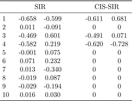
arm ibeh =n−1/(2+ri),i= 1,2,3. Dimension reduction methods SIR, CIS-SIR as well as their combining strategy are run separately, and their per-round regretrnis summarized in Figure 1 (right panel), which shows that the combining strategy performs the best. Since the second arm (i= 2) is played the most (for SIR, 1022 times; for CIS-SIR, 1026 times), we show the estimated dimension reduction matrix for the second arm at the last time point
n = N in Table 1. As expected, CIS-SIR results in a sparse dimension reduction matrix with rows 1, 3 and 4 being non-zero.
SIR CIS-SIR 1 -0.658 -0.599 -0.611 0.681
2 0.011 -0.091 0 0
3 -0.469 0.601 -0.491 0.071 4 -0.582 0.219 -0.620 -0.728
5 -0.001 0.075 0 0
6 0.071 0.232 0 0
7 0.013 -0.340 0 0
8 -0.019 0.087 0 0
9 -0.029 -0.194 0 0
10 0.016 0.030 0 0
Table 1: Comparing the estimated dimension reduction matrix ˆB2,N∗ for the second arm between SIR and CIS-SIR.
7. Web-Based Personalized News Article Recommendation
In this section, we use the Yahoo! Front Page Today Module User Click Log data set (Yahoo! Academic Relations, 2011) to evaluate the proposed allocation strategy. The complete data set contains about 46 million web page visit interaction events collected during the first ten days in May 2009. Each of these events has four components: (1) five variables constructed from the Yahoo! front page visitor’s information; (2) a pool of about 10-14 editor-picked news articles; (3) one article actually displayed to the visitor (it is selected uniformly at random from the article pool); (4) the visitor’s response to the selected article (no click: 0, click: 1). Since different visitors may have different preferences for the same article, it is reasonable to believe that the displayed article should be selected based on the visitor associated variables. If we treat the articles in the pool as the bandit arms, and the visitor associated variables as the covariates, this data set provides the necessary platform to test a MABC algorithm.
Another challenge in evaluating a MABC algorithm comes from the intrinsic nature of bandit problem: for every visitor interaction event, only one article is displayed, and we only have this visitor’s response to the displayed article, while his/her response to other articles is not available, causing a difficulty if the actually displayed article does not match the article selected by a MABC algorithm. To overcome this issue caused by limited feedback, we apply the unbiased offline evaluation method proposed by Li et al. (2010). Briefly, for each encountered event, the MABC algorithm uses the previous “valid” data set (history) to estimate the mean reward functions and propose an arm to pull. If the proposed arm matches the actually displayed arm, this event is kept as a “valid” event, and the “valid” data set (history) is updated by adding this event. On the other hand, if the proposed arm does not match the displayed arm, this event is ignored, and the “valid” data set (history) is unchanged. This process is run sequentially over all the interaction events to generate the final “valid” data set, upon which a MABC algorithm can be evaluated by calculating the click-through rate (CTR, the proportion of times a click is made). Under the fact that in each interaction event, the displayed arm was selected uniformly at random from the pool, it can be argued that the final “valid” data set is like being obtained from running the MABC algorithm over a random sample of the underlying population.
With the reduced data set and the unbiased offline evaluation method, we evaluate the performance of the following algorithms.
random: an arm is selected uniformly at random.
-greedy: The randomized allocation strategy is run naively without consideration of co-variates. A simple average is used to estimate the mean reward for each arm.
SIR-kernel: The randomized allocation strategy is run using SIR-kernel method to esti-mate the mean reward functions. Three sequences of bandwidth choices are consid-ered: hn1 =n−1/6,hn2 =n−1/8 and hn3 =n−1/10.
model combining: Model combining based randomized allocation strategy described in Section 3 is run with SIR-kernel method (hn3=n−1/10) and the naive simple average method (-greedy) as two candidate modeling methods.
The-greedy, SIR-kernel and model combining algorithms described above all take the first 1000 time points to be the forced sampling stage and use πn = n−1/4/6. Also, for any given arm, the SIR-kernel method limits the history time window for reward estimation to have maximum sample size of 10,000 (larger history sample size does not give us noticeable difference in performance). In addition, we consider the following parametric algorithm: LinUCB: LinUCB employs Bayesian logistic regression to estimate the mean reward
func-tions. The detailed implementation procedures are described in Algorithm 3 of Chapelle and Li (2011).
1.20
1.25
1.30
LinUCB ε-gre
edy
SIR-ke
rn
el-hn1
SIR-ke
rn
el-hn2
SIR-ke rn
el-hn3
mode l comb
ining
n
o
rm
al
ize
d
C
T
R
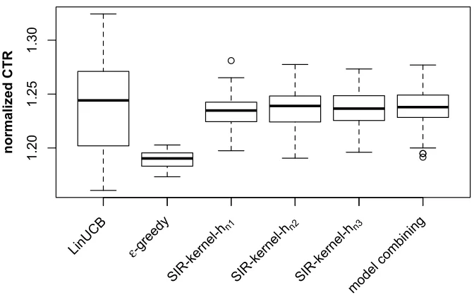
Figure 2: Boxplots of normalized CTRs of various algorithms on the news article recom-mendation data set. Algorithms include (from left to right): LinUCB, -greedy, SIR-kernel (hn1), SIR-kernel (hn2), SIR-kernel (hn3), model combining with SIR-kernel (hn3) and -greedy. CTRs are normalized with respect to the random algorithm.
It appears that the SIR-kernel methods with different candidate bandwidth sequences have very similar performance. The naive -greedy algorithm, however, clearly under-performs due to its failure to take advantage of the response-covariate association. When the naive simple average estimation (-greedy) is used together with SIR-kernel method (hn3) in the model combining algorithm, the overall performance does not seem to deterio-rate with the existence of this naive estimation method, showing once again that the model combining algorithm allows us to safely explore new modeling methods by automatically selecting the appropriate modeling candidate. Given that the covariates in the news article recommendation data set are constructed with logistic regression related methods (Li et al., 2010), it is satisfactory to observe that SIR-kernel algorithm can have similar performance with relatively small variation when compared with the LinUCB algorithm.
8. Conclusions
sub-optimal for the investigated randomized allocation strategy in the minimax sense (Perchet and Rigollet, 2013), the flexibility in estimation of the mean reward functions can be very useful in applications. In that regard, we integrate a model combination technique into the allocation strategy to share the strengths of different statistical learning methods for reward function estimation. It is shown that with the proposed data-driven combination of estimation methods, our allocation strategy can remain strongly consistent.
In Appendix A, we also show that by resorting to an alternative UCB-type criterion for arm comparison, the regret rate of the modified randomized allocation algorithm is improved to be minimax optimal up to a logarithmic factor. It remains to be seen if the UCB modification can be incorporated to construct a model combination algorithm with adaptive minimax rate. Moreover, as an important open question raised by a reviewer, it would be interesting to see whether the cumulative regret of the model combination strategy is comparable to that of the candidate model with the smallest regret in the sense of an oracle-type inequality similar to that of, e.g., Audibert (2009).
Acknowledgments
We would like to thank the Editor and two anonymous referees for their very constructive comments that help improving this manuscript significantly. This research was supported by the US NSF grant DMS-1106576
Appendix A. A Kernel Estimation Based UCB Algorithm
In this section, we modify the randomized allocation strategy to give a UCB-type algo-rithm that results in an improved rate of the cumulative regret. Similar to Section 4, we consider the Nadaraya-Watson estimation as the only modeling method, that is,
ˆ
fi,n(x) =
P
j∈Ji,nYi,jK
x−X
j hn−1
P
j∈Ji,nK
x−X
j hn−1
.
We slightly revise step 5 of the proposed randomized allocation strategy:
STEP 50. Estimate the best arm, select and pull. For the covariateXn, define ˜in= argmax
1≤i≤lfˆi,n(Xn) +Ui,n(Xn), (6)
where Ui,n(x) = ˜ c
s
(logN)P
j∈Ji,nK2
x−Xj hn−1
P
j∈Ji,nK
x−Xj hn−1
and ˜c is some positive constant (if there is a
tie, any tie-breaking rule may be applied). Choose an arm, with probability 1−(l−1)πn for arm ˜in (the currently most promising choice) and with probability πn for each of the remaining arms. That is,
In=
(
˜in, with probability 1−(l−1)πn,
Clearly, (6) shows a UCB-type algorithm that naturally extends from the UCB1 of Auer et al. (2002) and the UCBogram of Rigollet and Zeevi (2010). Indeed, given the uniform kernel K(u) = I(kuk∞ ≤ 1), we have Ui,n(x) = ˜c
q
logN
Ni,n(x), where Ni,n(x) is the number of times arm igets pulled inside the cube that centers atx with bin width 2hn−1. For presentation clarity, we assume K(·) is the uniform kernel, but the results can be generalized to kernel functions that satisfy Assumption 4. As shown in Theorem 4 below, the finite-time regret upper bound of the UCB-type algorithm achieves the minimax rate up to a logarithmic factor.
Theorem 4. Suppose Assumptions 0-1 hold and the uniform kernel function is used. Then for the modified algorithm, if n0 =lN hκ, ˜c >max{2
√
3v,12c}, h =hn = 1/d(logNN)
1 2κ+de
and πn≤ 1l ∧1c(lognN)
1
2+d/κ, the mean of cumulative regret satisfies
ERN(η)<C˜∗N1 − 1
2+d/κ(logN)
1
2+d/κ. (7)
It is worth noting that despite the seemingly minor algorithmic modification, the proof techniques used by Theorem 2 and Theorem 4 are quite different. The key difference is that: the UCB-type criterion enables us to provide upper bounds (with high probability) for the number of times the “inferior” arms are selected, and these bounds are dependent on the reward difference between the “optimal” and the “inferior” arms; for the algorithm before modification, we have to rely on studying the estimation errors of the reward functions and the UCB-type arguments do not apply. It is not settled yet as to whether the suboptimal rate of the -greedy type algorithm is intrinsic to the method or is the limitation of the proof techniques. But we tend to think that the rate given for the-greedy type algorithm is intrinsic to the method. Also, although the UCB-type algorithm leads to an improved regret rate, it is not yet clear how it could be used to construct a model combination algorithm.
Appendix B. Lemmas and Proofs
B.1 Proof of Theorem 1
Lemma 1. Suppose{Fj, j = 1,2,· · · }is an increasing filtration ofσ-fields. For eachj ≥1,
let εj be an Fj+1-measurable random variable that satisfies E(εj|Fj) = 0, and let Tj be an
Fj-measurable random variable that is upper bounded by a constant C >0 in absolute value almost surely. If there exist positive constants v and c such that for all k≥ 2 and j ≥ 1, E(|εj|k|Fj)≤k!v2ck−2/2, then for every >0 and every integer n≥1,
P
Xn
j=1
Tjεj ≥n
≤exp
− n
2 2C2(v2+c/C)
Proof of Lemma 1. Note that
P
Xn
j=1
Tjεj ≥n
≤e−tnE
h
exp
t
n
X
j=1
Tjεj
i
=e−tnEhEexp t
n
X
j=1
Tjεj
|Fni
=e−tnE
h
exp
t
n−1
X
j=1
Tjεj
E(etTnεn|Fn)
i
.
By the moment condition on εn and Taylor expansion, we have logE(etTnεn|F
n)≤E(etTnεn|Fn)−1
≤tTnE(εn|Fn) + ∞
X
k=2
tk|T n|k
k! E(|εn| k|F
n)
≤ v
2C2t2
2 (1 +cCt+ (cCt)
2+· · ·) = v
2C2t2 2(1−cCt)
fort <1/cC. Thus, it follows by induction that
P
n
X
j=1
Tjεj ≥n
≤exp−tn+ nv 2C2t2 2(1−cCt)
≤exp
− n
2 2C2(v2+c/C)
,
where the last inequality is obtained by minimization over t. This completes the proof of Lemma 1.
Lemma 2. Suppose{Fj, j = 1,2,· · · }is an increasing filtration ofσ-fields. For eachj ≥1,
letWj be anFj-measurable Bernoulli random variable whose conditional success probability
satisfies
P(Wj = 1|Fj−1)≥βj
for some 0≤βj ≤1. Then given n≥1,
P
Xn
j=1
Wj ≤ n
X
j=1
βj
/2
≤exp
−3
Pn
j=1βj 28
.
Proof of Lemma 2. Suppose ˜Wj, 1 ≤ j ≤ n are independent Bernoulli random variables with success probability βj, and are assumed to be independent of Fn. By Bernstein’s inequality (e.g., Cesa-Bianchi and Lugosi, 2006, Corollary A.3),
P
n
X
j=1 ˜
Wj ≤ n
X
j=1
βj
/2≤exp−3
Pn
j=1βj 28
.
Also,Pn
j=1Wjis stochastically no smaller thanPnj=1W˜j, that is, for everyt,P(Pnj=1Wj >
t) ≥P(Pn
j=1W˜j > t). Indeed, noting that P(Wn> t|Fn−1)≥ P( ˜Wn > t) for every t, we have
P(W1+· · ·+Wn> t|Fn−1)≥P(W1+· · ·+Wn−1+ ˜Wn> t|Fn−1).
Similarly, by P(Wn−1> t|Fn−2)≥P( ˜Wn−1 > t) for everytand the independence of ˜Wj’s,
P(W1+· · ·+Wn−1+ ˜Wn> t|Fn−2,W˜n)≥P(W1+· · ·+Wn−2+ ˜Wn−1+ ˜Wn> t|Fn−2,W˜n). Continuing the process above, we can see that P(Pn
j=1Wj > t)≥P(
Pn
j=1W˜j > t) holds.
Lemma 3. Under the settings of the kernel estimation in Section 4.1, given arm i and a cube A ⊂ [0,1]d with side width h, if Assumptions 0, 3 and 4 are satisfied, then for any >0,
Psup x∈A
X
j∈Ji,n+1 εjK
x−Xj
hn
> n
1−1/√2
≤ exp
− n
2 4c2
4v2
+ exp
− n
4c4c
+ ∞
X
k=1
2kdexp
−2
kn2
λ2v2
+ ∞
X
k=1
2kdexp
−2
k/2n 2λc
.
Proof of Lemma 3. At each time point j, let Wj = 1 if arm i is pulled (i.e., Ij =i), and
Wj = 0 otherwise. Denote G(x) = Pnj=1εjWjK(x −Xj
hn ). Then, to find an upper bound for P(supx∈AG(x) > n/(1−1/
√
2)), we use a “chaining” argument. For each k≥ 0, let
γk = hn/2k, and we can partition the cube A into 2kd bins with bin width γk. Let Fk denote the set consisting of the center points of these 2kd bins. Clearly, card(F
k) = 2kd, andFk is aγk/2-net ofAin the sense that for everyx∈A, we can find ax0 ∈Fk such that
kx−x0k∞≤γk/2. Let τk(x) = argminx0∈F
kkx−x
0k
∞ be the closest point to x in the net
Fk. With the sequence F0, F1, F2,· · · ofγ0/2, γ1/2, γ2/2,· · · nets inA, it is easy to see that for everyx∈A,kτk(x)−τk−1(x)k∞≤γk/2 and limk→∞τk(x) =x. Thus, by the continuity of the kernel function, we have limk→∞G(τk(x)) =G(x). It follows that
G(x) =G(τ0(x)) + ∞
X
k=1
G(τk(x))−G(τk−1(x))
Thus,
Psup x∈A
G(x)> n
1−1/√2
=P
sup x∈A
G(τ0(x)) + ∞
X
k=1
G(τk(x))−G(τk−1(x)) > ∞ X k=0 n 2k/2 ≤P sup x∈A
G(τ0(x))> n
+ ∞ X k=1 P sup x∈A
G(τk(x))−G(τk−1(x))
> n
2k/2
≤Psup x∈F0
G(x)> n+ ∞
X
k=1
P sup
x2∈Fk, x1∈Fk−1
kx2−x1k∞≤γk/2
G(x2)−G(x1)
> n
2k/2
≤card(F0) max x∈F0
P G(x)> n
+ ∞
X
k=1
2dcard(Fk−1) max x2∈Fk, x1∈Fk−1
kx2−x1k∞≤γk/2
P
G(x2)−G(x1)> n
2k/2
, (8)
where the last inequality holds because for each x1 ∈Fk−1, there are only 2d such points
x2 ∈Fk that can satisfykx2−x1k∞≤γk/2. Givenx∈F0, since|WjK(x −Xj
h )| ≤c4 almost surely for all j≥1, it follows by Lemma 1 that
P G(x)> n≤exp
− n
2 2c2
4(v2+c/c4)
. (9)
Similarly, givenx2∈Fk,x1∈Fk−1 and kx2−x1k∞≤γk, since
K
x2−Xj
hn
−Kx1−Xj hn
≤
λkx2−x1k∞
hn
≤ λγk
2hn = λ
2k+1 almost surely, it follows by Lemma 1 that
P
G(x2)−G(x1)> n
2k/2
=P
Xn
j=1
jWj
h
K
x2−Xj
h
−K
x1−Xj
h i > n 2k/2 ≤exp − 2
k+2n2 2λ2(v2+ 2k/2+1c/λ)
. (10)
Thus, by (8), (9) and (10),
P
sup x∈A
G(x)> n
1−1/√2
≤ exp− n
2 2c24(v2+c/c4)
+ ∞
X
k=1
2kdexp− 2
k+2n2 2λ2(v2+ 2k/2+1c/λ)
≤ exp− n
2 4c24v2
+ exp− n
4c4c
+ ∞
X
k=1
2kdexp−2
kn2
λ2v2
+ ∞
X
k=1
2kdexp−2
k/2n 2λc
.
Proof of Theorem 1. Recall thatMi,n =|Ji,n|,c is the covariate density lower bound, and
L, L1, c3 are constants defined in Assumption 4 for the kernel functionK(·), and. Note that for each x∈Rd,
|fˆi,n+1(x)−fi(x)|=
X
j∈Ji,n+1 Yi,jK
x−Xj
hn
X
j∈Ji,n+1 K
x−Xj
hn
−fi(x) = X
j∈Ji,n+1
(fi(Xj) +εj)K
x−Xj
hn
X
j∈Ji,n+1 K
x−Xj
hn
−fi(x) = X
j∈Ji,n+1
(fi(Xj)−fi(x))K
x−Xj
hn
X
j∈Ji,n+1 K
x−Xj
hn
+
X
j∈Ji,n+1 εjK
x−Xj
hn
X
j∈Ji,n+1 K
x−Xj
hn ≤ sup
{x,y:kx−yk∞≤Lhn}
|fi(x)−fi(y)|+
1
Mi,n+1hdn
X
j∈Ji,n+1 εjK
x−Xj
hn
1
Mi,n+1hdn
X
j∈Ji,n+1 K
x−Xj
hn , (11)
where the last inequality follows from the bounded support assumption of kernel function
K(·). By uniform continuity of the functionfi, lim
n→∞{x,y:kx−supyk ∞≤Lhn}
|fi(x)−fi(y)|= 0.
To show thatkfˆi,n−fik∞→0 asn→ ∞, we only need
sup x∈[0,1]d
1
Mi,n+1hdn
X
j∈Ji,n+1 εjK
x−Xj
hn
1
Mi,n+1hdn
X
j∈Ji,n+1 K
x−Xj
hn
→0 asn→ ∞. (12)
First, we want to show
inf x∈[0,1]d
1
Mi,n+1hdn
X
j∈Ji,n+1
Kx−Xj hn
> c3cL
d 1πn
2 , (13)
bins by ˜A1,A˜2,· · ·,A˜B˜. Given an armiand 1≤k≤B˜, for every x∈A˜k, we have
X
j∈Ji,n+1
Kx−Xj hn = n X j=1
I(Ij =i)K
x−Xj
hn ≥ n X j=1
I(Ij =i, Xj ∈A˜k)K
x−Xj
hn
≥c3 n
X
j=1
I(Ij =i, Xj ∈A˜k),
where the last inequality follows by Assumption 4. Consequently,
Pinf x∈A˜k
1
Mi,n+1hdn
X
j∈Ji,n+1
Kx−Xj hn
≤ c3cL
d 1πn 2
≤P
inf x∈A˜k
1
nhd n
X
j∈Ji,n+1 K
x−Xj
hn
≤ c3cL
d 1πn 2 ≤P c3 nhd n n X j=1
I(Ij =i, Xj ∈A˜k)≤
c3cLd1πn 2
=P
Xn
j=1
I(Ij =i, Xj ∈A˜k)≤
cn(L1hn)dπn 2
. (14)
Noting that P(Ij =i, Xj ∈A˜k|Zj)≥c(L1hn)dπj for 1≤j≤n, we have by Lemma 2 that
P
Xn
j=1
I(Ij =i, Xj ∈A˜k)≤
cn(L1hn)dπn 2
≤exp
−3cn(L1hn)
dπ n 28 . (15) Therefore, P inf x∈[0,1]d
1
Mi,n+1hdn
X
j∈Ji,n+1 K
x−Xj
hn
≤ c3cL
d 1πn 2 ≤ ˜ B X k=1 P inf x∈A˜k
1
Mi,n+1hdn
X
j∈Ji,n+1 K
x−Xj
hn
≤ c3cL
d 1πn 2
≤B˜exp−3cn(L1hn)
dπ n 28
,
where the last inequality follows by (14) and (15). With the conditionnh2dπ4n/logn→ ∞, we immediately obtain (13) by Borel-Cantelli lemma.
By (13), it follows that (12) holds if
sup x∈[0,1]d
1
Mi,n+1hdn
X
j∈Ji,n+1 εjK
x−Xj
hn
In the rest of the proof, we want to show that (16) holds. For each n ≥ n0l+ 1, we can partition the unit cube [0,1]d intoB bins with bin lengthhn such thatB ≤1/hdn. At each time pointj, letWj = 1 if arm iis pulled (i.e., Ij =i), andWj = 0 otherwise. Then given
>0,
P sup
x∈[0,1]d
1
Mi,n+1hdn
X
j∈Ji,n+1 εjK
x−Xj
hn
> πn
≤B max 1≤k≤BP
sup x∈Ak
1
Mi,n+1hdn
X
j∈Ji,n+1 εjK
x−Xj
hn
> πn
≤BP Mi,n+1 n ≤ πn 2
+B max 1≤k≤BP
sup x∈Ak
1
Mi,n+1hdn
X
j∈Ji,n+1 εjK
x−Xj
hn
> πn,
Mi,n+1 n > πn 2 ≤BP Mi,n+1 n ≤ πn 2
+B max 1≤k≤BP
sup x∈Ak
X
j∈Ji,n+1 εjK
x−Xj
hn
>
nπn2hdn
2
≤Bexp−3nπn
28
+B max 1≤k≤BP
sup x∈Ak
X
j∈Ji,n+1 εjK
x−Xj
hn
>
nπn2hdn
2
, (17)
where the last inequality follows by Lemma 2. Note that by Lemma 3,
Psup
x∈Ak
X
j∈Ji,n+1 εjK
x−Xj
hn
>
nπ2nhdn
2
≤P
sup x∈Ak
X
j∈Ji,n+1 εjK
x−Xj
hn
> nπ
2 nhdn
2
+Psup x∈Ak
X
j∈Ji,n+1
(−εj)K
x−Xj
hn
> nπ
2 nhdn
2
.
≤2 exp−( √
2−1)2nπn4h2dn 2
32c24v2
+ 2 exp−( √
2−1)nπn2hdn
8√2c4c
+ 2 ∞
X
k=1
2kdexp
−( √
2−1)22knπn4h2dn 2
8λ2v2
+ 2 ∞
X
k=1
2kdexp
−( √
2−1)2k/2nπn2hdn
4√2λc
. (18)
Thus, by (17), (18) and the condition that nh2dnπ4n/logn → ∞, (16) is an immediate consequence of Borel-Cantelli lemma. This completes the proof of Theorem 1.
B.2 Proofs of Theorem 2 and Corollary 2
Given x ∈ [0,1]d, 1 ≤i ≤ l and n ≥ n0l+ 1, define Gn+1(x) = {j : 1 ≤ j ≤ n,kx−
Lemma 4. Suppose Assumptions 0, 1 and 4 are satisfied, and{πn}is a decreasing sequence.
Given x∈[0,1]d, 1≤i≤l andn≥n0l+ 1, for every > ω(Lhn;fi),
PXn |fˆi,n+1(x)−fi(x)| ≥≤exp
−3Mn+1(x)πn
28
+ 4Nexp
−c
2
5Mn+1(x)πn −ω(Lhn;fi)
2
4c24v2+ 4c
4c −ω(Lhn;fi)
, (19)
wherePXn(·)denotes the conditional probability given design pointsXn= (X1, X2,· · ·, Xn).
Proof of Lemma 4. It is clear that if Mn+1(x) = 0, (19) trivially holds. Without loss of generality, assume Mn+1(x) >0. Define the event Bi,n ={M 1
i,n+1(x)
P
j∈Ji,n+1K(
x−Xj hn ) ≥
c5}. Note that
PXn |fˆi,n+1(x)−fi(x)| ≥
≤PXn
Mi,n+1(x)
Mn+1(x) ≤
πn 2
+PXn
|fˆi,n+1(x)−fi(x)| ≥, Mi,n+1(x) Mn+1(x) >
πn 2
≤exp−3Mn+1(x)πn
28
+PXn
|fˆi,n+1(x)−fi(x)| ≥,
Mi,n+1(x)
Mn+1(x) >
πn 2 , Bi,n
+PXn
|fˆi,n+1(x)−fi(x)| ≥,
Mi,n+1(x)
Mn+1(x)
> πn
2 , B c i,n
,
=: exp
−3Mn+1(x)πn
28
+A1+A2, (20)
where the last inequality follows by Lemma 2. UnderBi,n, by Assumption 4, the definition of the modulus continuity and the same argument as (11), we have
|fˆi,n+1(x)−fi(x)|=
P
j∈Ji,n+1Yi,jK
x−X
j hn
P
j∈Ji,n+1K
x−X
j hn
≤ω(Lhn;fi) +
1
c5Mi,n+1(x)
X
j∈Gi,n+1(x) εjK
x−Xj
hn
Define ˜σt = inf{n˜ : Pj=1n˜ I(Ij = iand kx−Xjk∞ ≤ Lhn) ≥ t}, t ≥ 1. Then, by the previous display, for every > ω(Lhn;fi),
A1 ≤ PXn
X
j∈Gi,n+1(x) εjK
x−Xj
hn
≥c5Mi,n+1(x) −ω(Lhn;fi)
, Mi,n+1(x) Mn+1(x)
> πn
2 ≤ n X ¯ n=0
PXn
¯ n X t=1
ε˜σtK
x−Xσ˜
t
hn
≥c5n ¯ −ω(Lhn;fi)
, Mi,n+1(x) Mn+1(x)
> πn
2 , Mi,n+1(x) = ¯n
≤
n
X
¯
n=dMn+1(x)πn/2e
PXn
¯ n X t=1
εσ˜tK
x−X˜σ
t
hn
≥c5¯n −ω(Lhn;fi)
≤
n
X
¯
n=dMn+1(x)πn/2e
2 exp− nc¯
2
5 −ω(Lhn;fi)
2
2c2
4v2+ 2c4c −ω(Lhn;fi)
≤ 2Nexp−c
2
5Mn+1(x)πn −ω(Lhn;fi)
2
4c2
4v2+ 4c4c −ω(Lhn;fi)
, (21)
where the last to second inequality follows by Lemma 1 and the upper boundedness of the kernel function. By an argument similar to the previous two displays (using the uniform kernel), it is not hard to obtain that
A2 ≤2Nexp
−Mn+1(x)πn −ω(Lhn;fi)
2
4v2+ 4c −ω(Lhn;fi)
. (22)
Combining (20), (21), (22) and the fact that 0 < c5 ≤ 1 ≤ c4, we complete the proof of Lemma 4.
Proof of Theorem 2. Since ˆfi∗(X
n),n(Xn)≤fˆˆin,n(Xn), the regret accumulated after the ini-tial forced sampling period satisfies that
N
X
n=n0l+1
f∗(Xn)−fIn(Xn)
= N
X
n=n0l+1 fi∗(X
n)(Xn)−fˆi∗(Xn),n(Xn) + ˆfi∗(Xn),n(Xn)−fˆin(Xn) +fˆin(Xn)−fIn(Xn)
≤
N
X
n=n0l+1
fi∗(X
n)(Xn)−fˆi∗(Xn),n(Xn) + ˆfˆin,n(Xn)−fˆin(Xn) +fˆin(Xn)−fIn(Xn)
≤
N
X
n=n0l+1
2 sup 1≤i≤l
|fˆi,n(Xn)−fi(Xn)|+AI(In6= ˆin)
. (23)
First, we find the upper bound of the estimation error regret. Given arm i,n≥n0l and
> ω(Lhn;fi),
P|fˆi,n+1(Xn+1)−fi(Xn+1)| ≥
≤EPXn+1
Mn+1(Xn+1)≤
cn(2Lhn)d 2
+EPXn+1
|fˆi,n+1(Xn+1)−fi(Xn+1)| ≥, Mn+1(Xn+1)> cn(2Lhn)
d 2
. (24)
Since for every x ∈ [0,1]d, P(kx−Xjk∞ ≤Lhn) ≥ c(2Lhn)d, 1 ≤j ≤n, we have by the extended Bernstein’s inequality that
PXn+1
Mn+1(Xn+1)≤
cn(2Lhn)d 2
≤exp−3cn(2Lhn)
d 28
. (25)
By Lemma 4,
PXn+1
|fˆi,n+1(Xn+1)−fi(Xn+1)| ≥, Mn+1(Xn+1)>
cn(2Lhn)d 2
≤exp−3cn(2Lhn)
dπ n 56
+ 4Nexp−c
2
5cn(2Lhn)dπn −ω(Lhn;fi)
2
8c2
4v2+ 8c4c −ω(Lhn;fi)
. (26)
Let
˜
i,n=ω(Lhn;fi) +
s
16c2
4v2log(8lN2/δ)
c25c(2L)dnhd nπn
.
Then, by (24), (25), (26) and the definition ofnδ in (3), it follows that for every n≥nδ,
P
|fˆi,n+1(Xn+1)−fi(Xn+1)| ≥˜i,n
≤ δ
4lN + δ
4lN + δ
2lN = δ lN,
which implies that
P
XN
n=nδ+1 2 sup
1≤i≤l
|fˆi,n(Xn)−fi(Xn)| ≥ N
X
n=nδ+1 2 max
1≤i≤l˜i,n−1
≤δ. (27)
Next, we want to bound the randomization error regret. Given > 0, since P(In 6= ˆin) = (l−1)πn, we have by Hoeffding’s inequality that
PA
N
X
n=nδ+1
I(In6= ˆin)− N
X
n=nδ+1
(l−1)πn
≥≤exp− 2
2
N A2
.
Taking =ApN/2 log(1/δ), we immediately get
P
A
N
X
n=nδ+1
I(In6= ˆin)≥A N
X
n=nδ+1
(l−1)πn+A
r N 2 log 1 δ
≤δ. (28)
B.3 Proof of Theorem 3
Lemma 5. Under Assumption E and the proposed allocation strategy, for each armi
Nt<∞ a.s. for all t≥1.
Proof of Lemma 5. It suffices to check that
∞
X
j=n0l+1
I(Ij =i) =∞ a.s.. (29)
Indeed, let Fn,n≥1 be theσ-field generated by (Zn, Xn, In). By the proposed allocation strategy, for allj≥n0l+ 1,
P(Ij =i|Fj−1)≥πj.
By Assumption E, P∞
j=n0l+1P(Ij = i|Fj−1) =∞. Therefore, (29) is an immediate result
of the L´evy’s extension of the Borel-Cantelli lemmas (Williams, 1991, pp.124).
Proof of Theorem 3. The key to the proof is to show kfˆi,n−fik∞ → 0 almost surely for 1≤i≤l (Yang and Zhu, 2002, Theorem 1). Without loss of generality, assume ∆ includes only two candidate procedures (m = 2). Given 1≤i≤l, assume that procedure δ1 ∈∆i1 and procedure δ2 ∈∆i2 (the case of δ1, δ2 ∈∆i1 is trivial). Since
kfˆi,n−fik∞=kWi,n,1( ˆfi,n,1−fi) +Wi,n,2( ˆfi,n,2−fi)k∞
≤Wi,n,1kfˆi,n,1−fik∞+Wi,n,2kfˆi,n,2−fik∞,
it suffices to prove that Wi,n,1
Wi,n,2 → ∞almost surely as n→ ∞.
As defined before, Nt = inf{n : Pnj=n0l+1I(Ij = i) ≥ t}, and let Fn be the σ-field
generated by (Zn, Xn, In). Then for any t≥1, Nt is a stopping time relative to {Fn, n≥ 1}. By Lemma 5, Nt < ∞ a.s. for all t ≥ 1. Therefore, the weights Wi,Nt,1, Wi,Nt,2 and the variance estimates ˆvi,Nt,1, ˆvi,Nt,2 and ˆvi,Nt for t ≥ 1 are well-defined. By the allocation strategy, the weight associated with arm i is updated only after this arm is pulled. Consequently, we only need to show Wi,Nt,1
Note that for any t≥1,
Wi,Nt+1,1 Wi,Nt+1,2
=Wi,Nt,1
Wi,Nt,2
׈v
1/2 i,Nt,2 ˆ
v1/2i,N
t,1
exp −( ˆfi,Nt,1(XNt)−Yi,Nt) 2−( ˆf
i,Nt,2(XNt)−Yi,Nt) 2 2ˆvi,Nt
!
=Wi,Nt,1
Wi,Nt,2
׈v
1/2 i,Nt,2 ˆ
v1/2i,Nt,1
×exp −( ˆfi,Nt,1(XNt)−fi(XNt)−εNt) 2−( ˆf
i,Nt,2(XNt)−fi(XNt)−εNt) 2 2ˆvi,Nt
!
=Wi,Nt,1
Wi,Nt,2
׈v
1/2 i,Nt,2 ˆ
v1/2i,N
t,1
exp ( ˆfi,Nt,2(XNt)−fi(XNt)) 2−( ˆf
i,Nt,1(XNt)−fi(XNt)) 2 2ˆvi,Nt
!
×exp εNt( ˆfi,Nt,1(XNt)−fˆi,Nt,2(XNt)) ˆ
vi,Nt
!
=Wi,Nt,1
Wi,Nt,2
׈v
1/2 i,Nt,2 ˆ
v1/2i,N
t,1
exp(T1t+T2t),
where
T1t=
( ˆfi,Nt,2(XNt)−fi(XNt)) 2−( ˆf
i,Nt,1(XNt)−fi(XNt)) 2 2ˆvi,Nt
,
and
T2t=
εNt( ˆfi,Nt,1(XNt)−fˆi,Nt,2(XNt)) ˆ
vi,Nt
.
Thus, for each T ≥1,
Wi,NT+1,1 Wi,NT+1,2
= T Y t=1 ˆ
v1/2i,N
t,2 ˆ
v1/2i,N
t,1 exp T X t=1
T1t+ T X t=1 T2t ! . (30)
Then define ξt =εNt( ˆfi,Nt,1(XNt)−fi(XNt)) and ξ
0
t =εNt( ˆfi,Nt,2(XNt)−fi(XNt)). Since
E(εNt|FNt) = 0, it follows by Assumption C, Assumption 0 and Lemma 1 that for every
τ >0 and every T ≥1,
P( T
X
t=1
ξt> T τ)<exp
− T τ
2 2c2
2(v2+cτ /c2)
.
Replacing τ by (log√T)b T τ
0, we obtain
T
X
t=1
ξt=o(
√
almost surely by Borel-Cantelli lemma. By the same argument, PT
t=1ξt0 =o(
√
T(logT)b) almost surely. Note that for each T ≥1,
ˆ
vi,NT+1,1 =
PT
t=1( ˆfi,Nt,1(XNt)−Yi,Nt) 2
T
=
PT
t=1( ˆfi,Nt,1(XNt)−fi(XNt)−εNt) 2
T
=
PT
t=1( ˆfi,Nt,1(XNt)−fi(XNt)) 2
T +
PT
t=1ε2Nt
T −
2PT
t=1ξt
T .
Similarly, for each T ≥1
ˆ
vi,NT+1,2 =
PT
t=1( ˆfi,Nt,2(XNt)−fi(XNt)) 2
T +
PT
t=1ε2Nt
T −
2PT
t=1ξt0
T .
By Assumption A and the previous two equations, we obtain that ˆ
vi,Nt,1 <vˆi,Nt,2 (31)
almost surely for large enought.
The boundedness of {ˆvi,Nt, t ≥ 1} as implied in Assumption D enables us to apply Lemma 1 again to obtain that
T
X
t=1
T2t=o(
√
T(logT)b), (32)
almost surely. By (31), (32) and Assumption A, we conclude from (30) that
Wi,NT+1,1 Wi,NT+1,2
→ ∞ a.s. asT → ∞.
This completes the proof of Theorem 3.
B.4 Proof of Theorem 4
Proof of Theorem 4. First, note that
RN(η) = N
X
n=1
f∗(Xn)−fIn(Xn)
I(In= ˜in) + N
X
n=1
f∗(Xn)−fIn(Xn)
I(In6= ˜in)
≤
N
X
n=1
f∗(Xn)−fIn(Xn)
I(In= ˜in,˜in6=i∗(Xn)) + N
X
n=1
AI(In6= ˜in)
= l
X
i=1 N
X
n=1
f∗(Xn)−fIn(Xn)
I In=i,˜in6=i∗(Xn),˜in=i
+ N
X
n=1
AI(In6= ˜in)
=: l
X
i=1 N
X
n=1