Biased randomly trapped random walks and applications to random walks on Galton Watson trees

(1)

warwick.ac.uk/lib-publications

A Thesis Submitted for the Degree of PhD at the University of Warwick

Permanent WRAP URL:

http://wrap.warwick.ac.uk/97359

Copyright and reuse:

This thesis is made available online and is protected by original copyright.

Please scroll down to view the document itself.

Please refer to the repository record for this item for information to help you to cite it.

Our policy information is available from the repository home page.

(2)

M A

O

D

C

S

Biased randomly trapped random walks

and applications to random walks on

Galton-Watson trees

by

Adam Bowditch

Thesis

Submitted for the degree of

Doctor of Philosophy

Mathematics Institute

The University of Warwick

(3)

Acknowledgments

First and foremost, my thanks go to my supervisor, David Croydon, for his support,

encouragement and many useful discussions throughout my PhD. Without his

con-tributions this work would not have been possible. I would also like to thank Jon

Warren and Roger Tribe for their suggestions and deliberation as part of my advisory

committee.

My thanks also go to Roger Tribe and Nina Gantert for a careful reading of

my thesis and many useful comments.

I also owe many thanks to everyone involved in the MASDOC doctoral training

centre, supported by EPSRC grant EP/HO23364/1, for their PhD course. In

partic-ular, I would like to thank Ben Lees and John Sylvester with whom I have discussed

many interesting problems relating to my field of research.

I would also like to thank the mathematics and statistics departments at the

University of Warwick for providing a fantastic environment and the opportunities this

has granted me. My thanks also go to the other establishments that have supported

me; in particular, the research institute for mathematical sciences at Kyoto University.

Finally, I would like to thank my friends and family for their continued support

and encouragement throughout my PhD. This includes, among others, the dodgeball

club at the University of Warwick who have given me some much needed respite and

(6)

Declarations

I declare that, to the best of my knowledge, the material in this thesis is original and

my own work, conducted under the supervision of David Croydon, except otherwise

indicated. Notably,

i) Chapter 3 is formed of work from Bowditch [24];

ii) Chapter 4 is formed of work from Bowditch [25];

iii) Chapter 6 contains work from two articles: Section 6.1 is formed from Bowditch

[26] and Section 6.2 is formed of work from Bowditch [25];

iv) Chapter 2 contains a range of results which appear in the articles noted above.

The material in this thesis is submitted to the University of Warwick for the

degree of Doctor of Philosophy and has not been submitted to any other university or

(7)

Abstract

In this thesis we study biased randomly trapped random walks. As our main

mo-tivation, we apply these results to biased walks on subcritical Galton-Watson trees

conditioned to survive. This application was initially considered model in its own

right.

We prove conditions under which the biased randomly trapped random walk

is ballistic, satisfies an annealed invariance principle and a quenched central limit

theorem with environment dependent centring. We also study the regime in which

the walk is sub-ballistic; in this case we prove convergence to a stable subordinator.

Furthermore, we study the fluctuations of the walk in the ballistic but sub-diffusive

regime. In this setting we show that the walk can be properly centred and rescaled so

that it converges to a stable process.

The biased random walk on the subcritical GW-tree conditioned to survive

fits suitably into the randomly trapped random walk model; however, due to a lattice

effect, we cannot obtain such strong limiting results. We prove conditions under which

the walk is ballistic, satisfies an annealed invariance principle and a quenched central

limit theorem with environment dependent centring. In these cases the trapping is

weak enough that the lattice effect does not have an influence; however, in the

sub-ballistic regime it is only possible to obtain converge along specific subsequences.

We also study biased random walks on infinite supercritical GW-trees with

leaves. In this setting we determine critical upper and lower bounds on the bias such

(8)

Chapter 1 Introduction

Over the last forty years random motions in random media have been intensively studied, resulting in the emergence of many new interesting phenomena, mathematical

models and probabilistic techniques. A large driving force in this work has been

due to a variety of probabilistic models originating from physical sciences including condensed matter physics, reaction kinetics and polymer dynamics where diffusion in

inhomogeneous media is of considerable interest (e.g. [12]). Specifically, models of

random traps are of particular interest in physical chemistry where many of the issues are closely linked to the analysis of the Schr¨odinger equation and random potentials

(see [39]).

A fundamental topic in the field of random walk in random environment is the evolution of the displacement of the walk from its origin and how it is influenced by

fluctuations in the environment. In a wide range of models of random walks in random

environments this is driven by a trapping mechanism where the randomness of the en-vironment creates adverse regions which slow the walk. In recent years there has been

much progress in models which involve trapping; a review of recent developments in a

range of models of directionally transient and reversible random walks on underlying graphs is given in [9].

As our main example we consider biased random walks on Galton-Watson

(GW) trees conditioned to survive. These trees consist of an infinite backbone with finite trees attached as branches. The branches form dead-ends in the environment

which makes it a natural setting for observing trapping as the walk is slowed by taking

excursions in the finite sections of the tree. The influence of the bias on the trapping is an important feature of the model; as the bias is increased the local drift away from

the root will increase but this does not necessarily speed up the walk. This is because it increases the time trapped in the finite leaves from which the walk cannot escape

without taking long sequences of movements against the bias.

(9)

length; see [74] and [77] for a more detailed history. In this model we consider a fixed

graph and sample an environment by randomly choosing the transition probabilities at each vertex independently from a fixed distribution. Trapping is caused by ‘bad

pockets’ in the environment which reverse the imposed drift thus slowing the walk.

Although some progress has been made in the generalised set-up (e.g. [47]), most work has focussed around usingZd(for d≥1) as the fixed underlying graph.

The one dimensional model received much attention in the 1970s; firstly in [70]

where conditions for transience and an expression for a limiting speed were determined and then in [50] where fluctuations and central limit theorems have been studied in

greater detail. There has also been a slightly more recent interest with large deviation

results having been determined in [30] and the case of the non-i.i.d. environment being considered in [3]. The renowned ‘environment viewed from the particle technique’

(introduced in [64] and developed in [29], [51]) acted as a major breakthrough for this

model and although the technique has been developed in a more general setting (see [68]) it has had little impact for higher dimensions.

More recently, the higher dimensional model has been studied in greater detail.

By using a renewal structure, a law of large numbers has been shown in [75] and, using a then new technique, functional central limit theorems have been proved in [21]. This

latter technique allows an annealed invariance principle to be extended to a quenched version when the dimension is sufficiently high. The technique is now sufficiently well

developed to be applied in a wide range of random walk models.

Another archetypal model in the field is that of random walk on supercritical percolation clusters. In this model we consider, for the environment, the unique infinite

cluster in supercritical Bernoulli bond percolation on Zd for d ≥ 2 (see [41] for an overview). This defines a random graph which, since there is positive probability that the cluster contains any fixed vertex, can be conditioned to contain the origin as a root

for the random walk. This is one of many natural examples which exhibit anomalous

behaviours caused by inhomogeneity in the environment.

One of the major features of the model is the occurrence of trapping; if we

introduce a weak bias then the walk moves at positive speed whereas if the bias is

strong then the speed vanishes (see [73]). This rather counter-intuitive behaviour occurs because, as the walker is pushed into new regions by the bias, it encounters

dead-ends that act as traps which hinder its escape from the root. The trapping

mechanism becomes stronger as the bias is increased because the greater bias makes it more difficult for the walk to escape the traps. This behaviour is very similar to

that of the random walk on GW-trees.

Both the isotropic and anisotropic walks have been studied in some detail with renormalisation and harmonic deformation techniques yielding rewarding outcomes. It

(10)

d ≥ 3 (but is centred and therefore clearly sub-ballistic). The anisotropic walk is

also transient in dimensiond≥2 (see [14] or [73]) and experiences a phase transition from ballistic to sub-ballistic as the bias is increased above the critical value which has

been identified in [37]. Moreover, regimes (both isotropic and anisotropic) such that

a functional central limit theorem holds have been determined in [13], [37] and [58]. The Bouchaud trap model was introduced in [22] in order to study aging

phe-nomenon in spin-glasses at low temperature. In this trapping model we randomly

assign a depth ωx to each vertex x of a graph; this forms the environment. For a

fixed environment, we then consider a continuous time random walk with independent

exponentially distributed holding times with mean ωx from site x. This model has

been discussed in great detail in the physics literature (e.g. [23], [61] and [69]) in the context of non-equilibrium phenomena in disordered systems.

A key feature in many of these physical models is aging in which the

decor-relation properties of the system are time dependent. This property of aging relates to localisation of the random walk in the Bouchaud trap model. Indeed, it has been

shown in [35] that, for the Bouchaud trap model on Z, if the depths belong to the domain of attraction of a stable law with index α < 1 (so that the depths ωx have

infinite mean) then the walk is subdiffusive and (suitably scaled) converges to the FIN

singular diffusion. This limit process is a Brownian motion time changed by the inverse of a stable subordinator evaluated at the local time of the Brownian motion (driven by

a speed measure associated with the environment). That is, the convergence is such

that the limit is environment dependent as the walk is slowed in areas of the graph with particularly deep traps.

The picture in higher dimensions is rather different. In this case we see, as

the limit, the fractional kinetics process (see [5], [8] and [63]). That is, a Brownian motion time changed by the inverse of a stable subordinator which is independent

of the Brownian motion. Specifically, the walk is slowed to the same extent but the

spatial aspect is insignificant because the walk never stays in one area for very long. This is, in fact, the same limit observed for the continuous time random walk with

infinite mean waiting time (see [59] and [62]). For a more detailed account we direct

the reader to [7] which gives a summary of mathematical results for the Bouchaud trap model in dimensionsd≥1 and also more detail in its relation to spin-glasses.

Recently, a more general model of randomly trapped random walks was

in-troduced in [6] to generalise models such as the Bouchaud trap model and provide a framework for studying random walks on other random graphs in which trapping

naturally occurs such as biased random walks on percolation clusters and random

walk in random environment. In this general model, rather than defining the trap at each vertex by a single variable (i.e. the depth), we randomly assign to each vertex

(11)

measures as the environment and then, for a fixed environment, consider a random

walk with independent holding times distributed according to the measure associated with the site at which the walk is positioned.

In the seminal paper [6] it is shown that the possible scaling limits of the

unbiased randomly trapped random walk onZbelong to a certain class of time changed Brownian motions called randomly trapped Brownian motions. This class of processes

includes both the fractional kinetics process and the FIN diffusion but also a much

larger class of processes called spatially subordinated Brownian motions in which the time change encodes the spatial inhomogeneity in a more intricate way than for the

FIN diffusion. Higher dimensional (d≥2) unbiased randomly trapped random walks

have been studied further in [27] where a complete classification of the possible scaling limits is given.

These random walk models are just a few of many instances of statistical

me-chanics in random media that are considered by physicists and mathematicians alike. Many of these act as a stepping stone for the understanding of more complicated

pro-cesses. For an overview of recent development for some such processes, including the

random walk on the incipient infinite cluster and other diffusion processes on fractals, we direct the reader to [52].

The remainder of this chapter will be used to introduce the main models we study throughout the thesis in greater detail. These models include the randomly

trapped random walk and biased random walks on subcritical and supercritical

GW-trees conditioned to survive. In Chapter 5 we will briefly consider several other models including the Bouchaud trap model. These will be used to demonstrate how the

randomness in the model influences the limiting behaviour and to conjecture results

for random walks on GW-trees. Because we view these models as a mechanism for studying random walks on GW-trees, we will not describe them in greater detail here,

leaving a more precise definition for Chapter 5. A slightly more detailed description of

the results we prove for each model is given in Sections 1.1 and 1.2 which describe the models; however, the precise statements of the theorems will always be given at the

beginning of the chapter. Throughout the thesis we will use many results for random

walks on fixed trees, random walks onZ, properties of stable laws and various other classical results. To avoid repetition and highlight some of the most important results,

we will state and prove a range of technical lemmas in Chapter 2.

In Chapter 3 we investigate biased RTRWs on Z and apply the results to random walks on subcritical GW-trees conditioned to survive. To begin, we prove

conditions under which the random walk is ballistic; that is, the walk has a positive

limiting speed. We then show that this speed satisfies an Einstein relation; more specifically, that the derivative of the speed (with respect to the bias) converges to

(12)

used to centre the random walk in order to prove an annealed functional central limit

theorem; namely, we consider a renewal argument similar to that of [72] to prove that the position of the walk can be centred and rescaled so that the process converges in

distribution to a Brownian motion. We then adapt a technique used in [40] to derive a

quenched central limit theorem with an environment dependent centring. We conclude the chapter by applying these results to biased random walks on subcritical GW-trees

conditioned to survive.

In Chapter 4 we study biased random walks on subcritical GW-trees condi-tioned to survive in the sub-ballistic regime. Briefly, the sub-ballistic regimes splits

into four phases depending on the bias and the stability of the offspring law. We will

discuss these phases in greater detail after a more precise definition of the tree. In one of the phases we have that the walk is recurrent and we do not study this further. In

the other three sub-ballistic phases the walk is transient but slowed due to

character-istics of the tree. In each of these cases we determine the correct polynomial scaling such that the walker’s distance from the root converges to some non-trivial limit.

In Chapter 5 we consider the randomly trapped random walk in the

sub-diffusive regime; that is, when the trapping is too strong to obtain a central limit theorem. This splits into two distinct phases depending on whether the holding times

have finite mean. When the expected holding time is infinite we have that the walk is sub-ballistic. In this general setting we give conditions under which the position of the

walk converges, after suitable rescaling, to the inverse of a stable subordinator. This

is not possible for the random walk on the subcritical GW-tree because of a so-called lattice effect which we will explain in greater detail in Section 1.2.2. The other phase

we consider is where the holding times have finite mean but infinite variance. In this

setting we are able to apply the speed result from Chapter 3 but the fluctuations are too large to obtain a central limit theorem. Here, we prove a condition which shows

that, under suitable centring and rescaling, the walk converges in distribution to a

stable process. We then apply these results to some of the classical models of random walks in one-dimensional random environments; most notably the comb model which

can be seen as a logical intermediary for the study of random walks on subcritical

GW-trees.

In Chapter 6 we move onto random walks on supercritical GW-trees conditioned

to survive. Unlike the random walk on the subcritical GW-tree conditioned to survive,

this model does not easily fit into the randomly trapped random walk model. Despite this, we are able to use many estimates for trapping times proved throughout the

thesis alongside existing framework (due to [10], [55] and [65] among others) in order

to prove new results. In particular, we extend a result from [65] to prove a quenched functional central limit theorem and develop a result from [10] concerning the correct

(13)

Throughout the thesis we have used a large amount of notation, some of which

varies between chapters. We include a note on the notation used and a list of the important, frequently used notation in the glossary.

1.1 Randomly trapped random walks

We next introduce the general RTRW model in more detail. Fix a graphG=G(V, E) and let (Yk)k≥0 be a random walk on G with a lawP. Forx∈V write

L(x, n) :=

n

X

k=0

1{Yk=x}

for the local time of Y at site x by time n. We define a random environment ω

as a sequence of (0,∞)-valued probability measures (ωx)x∈V with environment law

P:=π⊗V for a fixed lawπ. For a fixed environmentω, let (ηx,i)x∈V,i≥1be independent

withηx,i∼ωx. Writing

Sn :=

X

x∈V

L(x,n−1) X

i=1

ηx,i = n−1 X

k=0

ηYk,L(Yk,k) and S

−1

t := inf{k≥0 :Sk> t}

we then define the randomly trapped random walk by

Xt:=Y_S−1

t .

This process is then a continuous time random walk onGwithkth holding timeηk :=

ηYk,L(Yk,k) and we writeη:= (ηk)k≥0 to be the sequence of holding times. That is, for

a fixed environmentω and walkY, the random variablesηkfork≥0 are independent

with lawωYk. For convenience we will defineSt=Sbtcwherebtc:= max{k∈Z:k≤t}

for non-integert∈R. We let Pω denote the law over X for the fixed environment ω andP(·) :=R Pω(·)P(dω) the annealed law.

This model was first introduced in [6] primarily to study the case in which the

embedded walk (Yk)k≥0 is a simple, symmetric random walk on Z. This setting is used to develop the foundations and gain some understanding of the possible scaling

limits that arise in this general model. It is shown that the scaling limits belong to

a large class of time changed Brownian motions (called randomly trapped Brownian motions) where the time change may retain much of the randomness of the spatial

inhomogeneity. This includes the FK-process, the FIN diffusion and also a new class

of processes called spatially subordinated Brownian motions which are time changes of Brownian motions where the time change reflects the randomness of the spatial

(14)

process and a spatially subordinated Brownian motion.

In [27], the model in which the embedded walk is a genuinely d-dimensional centred random walk onZd(ford≥2) with finite range jump distribution is studied. In this setting, it is shown that the only scaling limits are the constant time changed

Brownian motion and the fractional kinetics process. That is, the limiting process is independent of the spatial randomness because the embedded walk does not spend

a significant amount of time in any area of the graph. This generalises previously

well known results for models such as the continuous time random walk [59] and the Bouchaud trap model [8]. These results for the general model of randomly trapped

random walk are in the annealed setting whereas, in many cases, quenched results

are known for specific models; for instance, the Bouchaud trap model [36], [63]. It should be the case that the annealed convergence to Brownian motion extends to a

quenched result in high enough dimension by using the technique developed in [21].

The reason for this is that the randomness of the embedded walk creates a mixing in the environment which results in no specific trap (or ‘small’ collection of traps) having

a significant impact on the fluctuations. We consider this approach later when we

investigate random walks on supercritical GW-trees.

In this thesis we consider the randomly trapped random walk model in which

the embedded walk (Yk)k≥0 is a simple, biased random walk on Z. That is, we write Yk := Pkj=1χj for a sequence of i.i.d. random variables (χj)j≥1 satisfying P(χj =

−1) = (β+ 1)−1 = 1−P(χj = 1). This model will be the main focus of Chapters

3 and 5. Although we have the same underlying graph as studied in [6], we do not observe time changes which retain the randomness of the spatial composition in the

same way. The reason for this is that the bias constantly forces the walk into new

regions of the graph making it unlikely that the walk spends a large amount of time in any finite region. The walk is, therefore, transient and in many ways behaves somewhat

similarly to the walk in a higher dimensional graph. The main exception to this is

that the walk can only escape along a single path; this means that, in the quenched setting, the fluctuations of the walk are, in part, driven by the specific inhomogeneity

in the environment.

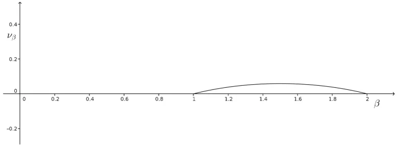
In Chapter 3 we prove a law of large numbers and two central limit theorems for the randomly trapped random walk onZ. That is, in Theorem 3.1, we show that if the bias is positive (β >1) and the expected holding timeη0 (underP) is finite, then Xnt/n convergesP-a.s. to the deterministic process νβtwhere νβ is a known constant

(called the speed). We then show that this speed satisfies an Einstein relation; more

specifically,

lim

β→1+

d dβνβ =

Υ 2

(15)

states that, ifβ >1 and E[η02]<∞ then for someς ∈(0,∞)

B_tn:= Xnt−ntνβ ς√n

converges in P-distribution to a Brownian motion. We prove this by considering a renewal argument similar to that of [72].

For the final CLT result for the RTRW, we adapt the technique used in [40] (to prove a quenched CLT for a random walk in random environment) to derive a quenched

central limit theorem with an environment dependent centring (Theorem 3.3). That

is, we show that ifβ >1, E[η02]<∞ and for someε >0 thatE[Eω[η0]2+ε]<∞ then

there existsϑ∈(0,∞) such that forP-a.e. ω there exists an environment dependent centringGω_{(n) such that}

Xn− Gω(n)

ϑ√n

converges in distribution to a standard Gaussian. In particular, we show that the known function Gω_{(n) can be written as the annealed, deterministic centring with}

an environment dependent correction where this correction is a sum of centred i.i.d.

random variables (with non-zero variance) under the environment law. This shows that the correction obeys a central limit theorem under P which means that it has √

n fluctuations and is, therefore, necessary.

A quenched central limit theorem has not been proved for the randomly trapped random walk in Zd for d≥2 although it has been shown in [27] that, for the unbi-ased walk, ifE[η0]<∞thenXntn−1/2 converges in distribution to a scaled Brownian

motion under the annealed law. Using the technique developed in [21] it should be possible to extend this to a quenched result in dimension d≥4 without the need for

an environment dependent centring; similarly, this should also hold for the unbiased

case. In dimensions d ≤ 3 the technique cannot be applied because it relies on two independent copies of the walk not visiting the same vertices at large times. By

com-parison with the Bouchaud trap model (see [7]) we expect that a quenched functional

central limit theorem should still hold (at least in the unbiased case) ford= 2,3. In Chapter 5 we consider the randomly trapped random walk when the trapping

is too strong to obtain a central limit theorem. In this setting there are two distinct

phases depending on whether E[η0]<∞. In both cases we prove functional limiting

results for the position of the walk.

When E[η0] = ∞ we have that the walk is sub-ballistic. In this setting, our

main result is Theorem 5.1 in which we show that if β >1, there exists an regularly

varying with index 1/αfor some α∈(0,1) and for anyk∈_Nand some functionf we have that

−nlog E

"

Eω

exp

λη0

an

k#!

(16)

thenXant/n converges inP-distribution to the inverse of anα-stable subordinator.

The other phase we consider is whereE[η0]<∞butE[η02] =∞. In this setting

we are able to apply the speed result from Chapter 3 but the fluctuations are too

large to obtain a central limit theorem. The aim of this case is to prove Theorem 5.2.

Here, we show that ifβ >1, there existsanregularly varying with index 1/αfor some

α∈(1,2) and for any k∈_Nand some function f we have that

nlog E

"

Eω

exp

λ(η0−E[η0])

an

k#!

∼f(k)λα

then (Xnt−ntνβ)/an converges in P-distribution to a stable process with indexα. These two asymptotic conditions for the sub-diffusive regimes appear to be

quite technical however they relate to the usual stable law conditions (as we discuss

in Chapter 5) and are, in fact, quite applicable as we shall show in a range of exam-ples. Importantly, these conditions only depend on a single excursion. This makes

dealing with the quenched law much more straightforward since we no longer need to

understand the correlation between the number of times traps are entered.

1.2 Random walks on trees

Our main motivation for investigating the randomly trapped random walk model is the study of biased random walks on GW-trees conditioned to survive. A GW-tree

conditioned to survive consists of an infinite backbone with finite trees attached as

branches. These branches form dead-ends in the environment which makes it a natural setting for observing trapping as the walk is slowed by taking excursions in the branches

of the tree.

In this section we introduce the general framework of random walks on trees with particular focus on GW-trees. We then briefly describe the main results that

we later prove for these models. By a tree we mean a rooted, locally finite graph T which contains no cycles and we let d be the graph distance metric on T. We denote by ρ the root and refer to the collection of vertices of graph distance k from

ρ as the kth generation of the tree. For vertices x, y ∈ T which are neighbours

(i.e. d(x, y) = 1) we say that x is the parent of y (equivalently y is a child of x) if d(ρ, x) =d(ρ, y)−1; that is,xbelongs to the generation beforey. We then letc(x) be

the set of children ofxand←−y to be the unique parent ofy(wheny6=ρ). We say that

y is a descendant of x (equivalentlyx is an ancestor of y) if the unique self-avoiding path betweenρ and y passes throughx. We then denote by Tx the maximal subtree

formed by the descendants ofx (where we consider Tx to be rooted atx). We define

H(T) := sup{d(ρ, x) :x∈T}to be the height of the tree T.

(17)

random walk on T is a random walk (Xn)n≥0 on the vertices of T which is β-times

more likely to make a transition to a given child of the current vertex than the parent (which are the only options). More specifically, the random walk started fromz∈T

is the Markov chain defined byP_zT(X0 =z) = 1 and the transition probabilities

P_zT(Xn+1 =y|Xn=x) =

       

      

1

1+β|c(x)|, ify=

←−_{x ,}

β

1+β|c(x)|, ify∈c(x), x6=ρ,

1

|c(ρ)|, ify∈c(x), x=ρ, 0, otherwise.

We useP(·) :=RPρT(·)P(dT) for the annealed law obtained by averaging the quenched

law P_ρT over a law P on random rooted trees. Unless indicated otherwise, we start the walk atρ.

Forx∈T, let|x|:=d(ρ, x) denote the distance between xand the root of the tree. Our principle interest will be the evolution of |Xn| with respect to both P and

PT.

We next briefly describe GW-processes and the GW-trees which arise from them; for further detail see, for example, [44]. Let {pk} denote a probability

distri-bution on Z+,f(s) :=Pk≥0pksk its probability generating function and ξ a random

variable with this law. To avoid trivial cases we assume thatp0+p1 <1. We consider

a GW-process with offspring distribution ξ as the Markov chain (Zn)n≥0 describing

the generation sizes of a branching process started from a single progenitor (Z0 = 1)

where each individual independently gives rise to a random number (distributed with

respect tof) of offspring in the next generation. That is,

Zn+1 =

Zn

X

j=1

ξn,j

where{ξn,j :n≥0, j ≥1} are independent copies ofξ. Let µ:=E[ξ] be the mean of

the offspring distribution which we assume to be finite andσ2 := VarP(ξ) which may

be infinite. (In fact, so that the asymptotic (2.9) holds, we make the slightly stronger assumption throughout that E[ξlog+(ξ)] <∞.) This process gives rise to a random treeTf _{where individuals are represented by vertices, edges connect individuals with}

their offspring and we identify the unique progenitor with the rootρ.

We write q for the extinction probability of Zn; that is, the probability that

Zn= 0 eventually. It is classical (e.g. [4, Section I.5]) thatq <1 if and only if µ >1;

that is, ifµ≤1 then the process dies out P-a.s. and, otherwise, there is some positive probability that the process survives forever. We refer to the three casesµ <1,µ= 1

(18)

1.2.1 Random walks on supercritical Galton-Watson trees

As previously mentioned, a supercritical GW-tree comes from a GW-process whose

offspring distribution has mean µ > 1 and, therefore, there is a positive probability

that the tree survives for infinitely many generations. We will work on these trees and denote byT a random tree with the law ofTf _{conditioned on survival.}

We next briefly describe the supercritical GW-tree conditioned on survival

following [4, Section I.12] and [44]. We define

g(s) := f(s)−f(qs)

1−q and h(s) := f(qs)

q

which are generating functions of GW-processes. In particular, g is the generating function of a GW-process without deaths and h is the generating function of a

sub-critical GW-process. Anf-GW-tree conditioned on nonextinctionT can be generated

by first generating ag-GW-treeTg _{and then, to each vertex}_x_of_Tg_{, appending a}

ran-dom numberM_xof independenth-GW-trees. We refer toY :=Tg_{as the backbone of}

T, the finite trees appended toY as the traps and the vertices in the first generation

of the traps as the buds. The distribution ofMx depends on the backbone locally; we

will not use the exact form but we include it here for brevity. Specifically, letcg(x) be

the offspring ofx inTg _{then the distribution of}_M

x conditional on Tg can be defined

by its probability generating function:

E

sMx_|Tg

= f

(|cg(x)|)_(qs)

f(|cg(x)|)_(q)

wheref(k) denotes thekth derivative of f.

It has been shown in [55] that if β ∈ (µ−1, f0(q)−1) then |Xn|n−1 converges

P-a.s. to a deterministic constant νβ > 0 called the speed of the walk. We refer

to this as the ballistic regime. When β < µ−1 the walk is recurrent and |Xn|n−1

converges P-a.s. to 0. This occurs because the backbone has average degree µ and, therefore, the embedded walk on the backbone only has drift away from the root

when β > µ−1. When the bias is large the walk is transient but slowed by having to make long sequences of movements against the bias in order to escape the traps; in

particular, ifβ ≥f0(q)−1 then the slowing effect is strong enough to cause|Xn|n−1 to

convergeP-a.s. to 0. We refer to this as the sub-ballistic regime.

In the ballistic regime |Xn|n−1 converges P-a.s. to a deterministic constant νβ >0; in this case it is natural to study the fluctuations. For ς, t >0 andn= 1,2, ...

define

B_tn:= |Xbntc| −ntνβ ς√n .

(19)

exponen-tial moments then for anyβ > µ−1 there existsς >0 such that, for P-a.e. treeT, the process (B_tn)t≥0 converges in PT-distribution to a standard Brownian motion. This

no longer requires the ballisticity condition β < f0(q)−1 _{which is due to the trapping}

in the dead-ends caused by the leaves. Indeed, whenp0 = 0 we have that q = 0 and

f0(0) = 0 therefore the condition becomes irrelevant. This regime is studied further to the case where β = µ−1 and p0 = 0; in this setting νβ = 0 and it is shown that

(B_tn)t≥0 converges inPT-distribution to the absolute value of a Brownian motion.

This result is extended in [31] to random walks on multi-type GW-trees with leaves. That is, the offspring distribution at each vertex is chosen randomly (depending

on the past) from some finite alphabet and the bias is fixed as the inverse of the

Perron-Frobenius eigenvalue for the matrix of expected offspring numbers. In this way the walk has zero drift along the backbone P-a.s. Although the dead-ends in this model trap the walk, the bias is small and therefore the slowing is weak.

It has been hypothesized in [9, Conjecture 3.1] that if the offspring law has deaths (p0 > 0) then, for any β ∈ (µ−1, f0(q)−1/2) and P-a.e. tree T, the process

(B_tn)t≥0 should converge in PT-distribution to a standard Brownian motion. By

choosingp0 >0, we allow the tree to have leaves; this creates traps in the environment

which slow the walk. We then require this additional upper bound on the bias so that

the trapping times have finite variance. We prove this conjecture in Section 6.1 and conclude that this upper bound on the bias is sharp.

In the sub-ballistic phase,β > f0(q)−1, it has further been observed in [10] that

if the offspring distribution has finite variance, then the walker follows a polynomial escape regime. In Section 6.2 we show that this regime extends to the case where the

offspring distribution belongs to the domain of attraction of a stable law with index

α∈(1,2).

We shall see that the finite branches are typically quite short and the

embed-ded walk on the backbone does not deviate too far from the furthest point reached;

we therefore have a strong relation between |Xn| and the time ∆n := inf{m ≥ 0 :

Xm ∈ Y,|Xm| = n} taken to reach the nth generation of the backbone. The time

∆n mainly consists of the duration of excursions in the deepest branches. Due to the

transience of the walk we have that the amount of time spent in these deep branches are asymptotically independent. It follows that ∆n can be approximated by the sum

of i.i.d. copies of the time spent in independent large branches.

We show further that only the height H of the branch, and not the foliage, contributes to the scaling. By comparison with the model in which we strip all of the

branch except the unique self-avoiding path to the deepest point, by transience the

walk reaches the deepest point with positive probability and then takes a geometric number of short excursions with escape probability close to β−H. In particular, this

(20)

The height H is approximately geometric with parameter f0(q); we therefore

see branches of height approximately log(n)/log(f0(q)−1) by generation n. In par-ticular, the time spent in the largest branch up to generation n will cluster around

βlog(n)/log(f0(q)−1)≈n1/γ where we define the exponent γ := log(f

0_(q)−1₎

log(β) . (1.1)

We then have that ∆nn−1/γ converges in distribution, with respect toP, along subse-quences of the formnl(t) =btf0(q)−lc. This shows that |Xn|scales with nγ.

It is natural to consider whether this result can be extended to show that |Xn|n−γ converges more generally. It has been shown in [10] that this is not the case

due to a certain lattice effect. That is, since H is approximately geometric we have that βH will not belong to the domain of attraction of any stable law therefore ∆n

only converges along specific subsequences. A related model is studied in [11] and [43]

where the conductance along each edge is chosen randomly according to a distribution satisfying a certain non-lattice assumption. In this setting the tail of the trapping

times obey a pure power law and the rescaled walk converges in distribution.

We will not study the regime whereβ∈(f0(q)−1/2, f0(q)−1) here. In this regime the walk has a positive speedνβ but the slowing is too strong to obtain a central limit

theorem. Heuristically, we expect that |Xn−nνβ| ' n1/γ where γ is the exponent

defined in (1.1). However, due to the same lattice effect seen in the sub-ballistic regime, we would only expect to observe convergence along suitably chosen subsequences.

1.2.2 Random walks on subcritical Galton-Watson trees

Similarly to the supercritical GW-tree conditioned to survive, a subcritical GW-tree conditioned to survive consists of an infinite backbone with finite trees attached as

branches. These branches are formed of collections of subcritical GW-trees as in the

supercritical case however, the backbone consists of a semi-infinite path emanating from a fixed root vertex. In particular, the branches of the subcritical tree are i.i.d.

and very similar in structure to those of the supercritical tree. For this reason,

study-ing random walks on the subcritical tree is a natural tool for studystudy-ing the trappstudy-ing mechanism of random walks on the supercritical tree without the added complications

which arise from the backbone of the supercritical tree. The study of random walks

on subcritical trees is largely motivated by the study of random walks on supercrit-ical trees; despite this, we will see that the subcritsupercrit-ical tree exhibits various unusual

characteristics which are not seen on the supercritical tree and give rise to interesting asymptotic properties for the walk.

The branches of the subcritical trees are typically very short and the embedded

(21)

in Section 2.5 that a random walk on a subcritical GW-tree conditioned to survive can

be coupled to a randomly trapped random walk so that the two walks do not deviate too far from each other. We therefore use random walks on subcritical GW-trees

conditioned to survive as our main motivation for studying one-dimensional randomly

trapped random walks.

We now describe subcritical GW-trees conditioned to survive following [2], [46]

and [49]. Unlike the supercritical GW-tree, the unconditioned subcritical GW-tree dies

outP-a.s. and therefore,a priori, we cannot discuss subcritical GW-trees conditioned to survive without first questioning their existence. It has been shown in [49] that

there is a well defined probability measure overf-GW trees conditioned to survive for

infinitely many generations which arises as a limit of probability measures overf-GW trees conditioned to survive at leastn generations. It is this distribution we consider

and we denote byT a tree with this law.

Recall that the offspring law of the process is given byP(ξ=k) =pk, we then

define the size-biased distribution by the probabilitiesP(ξ∗ =k) =kpkµ−1. It can be

seen (e.g. [46]) that the subcritical GW-tree conditioned to survive coincides with a

construction of a random tree with two types of vertex which we refer to asnormal and

special vertices. Start with a single special vertex in generation 0. At each generation

let every normal vertex give birth onto vertices according to independent copies of the offspring distribution and (independently) every special vertex give birth onto vertices

according to independent copies of the size-biased distribution. We then choose one

child of each special vertex uniformly at random to be special. All remaining vertices (children of either normal or special vertices) are then labelled as normal. We must

have a unique special vertex in each generation because we start with a single special

vertex and each special vertex gives birth to precisely one special vertex.

Unlike the supercritical tree which has infinitely many infinite paths, the

back-boneY of the subcritical tree conditioned to survive consists of a unique semi-infinite

path from the initial vertex ρ. Specifically, Y is formed of the special vertices in the construction. As for the supercritical tree, we refer to those vertices not on Y

which are children of vertices on Y as buds and the finite trees rooted at the buds

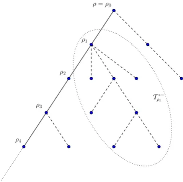
as traps. We write ρi for the unique vertex on Y which is distance i from ρ and

T∗−

ρi := Tρi \ Tρi+1 as the branch emanating from ρi. Due to the one dimensional

backbone, this model easily fits into the randomly trapped random walk framework

and as such it will be convenient to consider the walk as a trapping model. To this end, we define the embedded walk (Yk)k≥0 given by Yk := XSk where S0 := 0 and

Sk:= inf{m > Sk−1: Xm, Xm−1∈ Y}fork≥1. This means that Y makes the same

transitions along the backbone asX but does not experience the traps.

Before describing our results for random walks on subcritical GW-trees

(22)

[image:22.595.224.408.109.291.2]

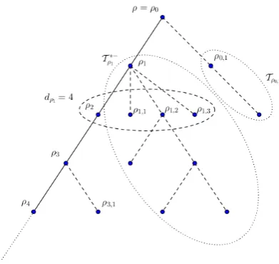
Figure 1.1: A sample subcritical GW-tree conditioned to survive T with the backbone Y

represented by solid lines and the buds and traps connected by dashed lines.

GW-trees conditioned to survive. The most obvious difference is the structure of the

backbone. In the subcritical case we have a semi-infinite path emanating from a fixed root and in the supercritical case we have a random tree. This means that dealing with

the embedded walk in the subcritical case is far easier however it will also give rise to

interesting phenomena when we study quenched central limit theorems in Chapter 3. Another key difference is the distribution over the buds. In the subcritical case,

the number of buds had a size-biased law independent of the position on the backbone.

In the supercritical case, the distribution over the number of buds is more complicated since it depends on the backbone. Importantly, in the supercritical case, the expected

number of buds can be bounded above byµ(1−q)−1 independently of higher moments

of the offspring law. This is not true in the subcritical case. In particular, if ξ has infinite second moments thenξ∗ has infinite mean. This will be important in Chapter

4 where we will observe rich behaviour in the subcritical case (when the offspring law

has finite mean but infinite variance) which is not present in the supercritical case. A final noteworthy difference is the offspring distribution of the traps. Recall

that in both cases the buds are roots of subcritical GW-trees. In the subcritical case

the law over these trees is the same as the original offspring law. In the supercritical case the law coincides with that of the supercritical GW-process conditioned to die

out; in particular, it is governed by h. Letting ξh denote a variable with this law we have thatP(ξh =k) =pkqk−1 and therefore ξh has exponential moments.

When the offspring law has finite variance, the limiting behaviour of |Xn| on

(23)

phenomenon of deep traps. When the offspring law has infinite variance, the bud

distribution of the subcritical tree has infinite mean which causes an extra slowing effect which is not seen with the supercritical tree. This equates for the different

exponents observed in the two models as shown in Figure 1.2. The walk on the critical

tree experiences a similar trapping mechanism to the subcritical tree; however, the slowing is more extreme and belongs to a different universality class which had been

shown in [28] to yield a logarithmic escape rate.

The first order scaling limits that can occur in the subcritical case are as follows. There exists a limiting speed νβ such that |Xn|/n converges P-a.s. to νβ under P; moreover, the walk is ballistic if and only if 1< β < µ−1 andσ2 <∞. We prove this

in Chapter 3 by comparison with the randomly trapped random walk. In fact, we are able to prove the following explicit expression for the speed:

νβ =

µ(β−1)(1−βµ)

µ(β+ 1)(1−βµ) + 2β(σ2₋_µ(1₋_µ)).

Such an expression is not known in the supercritical case; however, a description of

the invariant distribution of the environment seen from the particle is used in [1] to

give an expression of the speed in terms of an annealed expectation.

The sub-ballistic regime has four distinct phases. When β ≤ 1 the walk is

recurrent and we are not concerned with this case here; we study the remaining three

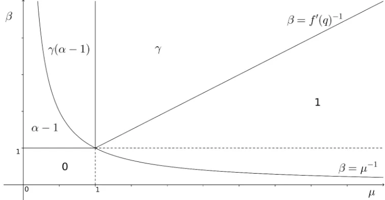
cases in Chapter 4. Figure 1.2 is the phase diagram for the almost sure limit of log(|Xn|)/log(n) (which is the leading order polynomial exponent in the scaling of

|Xn| relative to β and µ) where the offspring law has stability index α (which is 2

when σ2 <∞). Strictly,f0(q) is not a function of µ therefore the lineβ =f0(q)−1 is not well defined; Figure 1.2 shows the particular case when the offspring distribution

belongs to the geometric family. It is always the case that f0(q) <1 therefore some

such ballistic region always exists however the parametrisation depends on the family of distributions.

As in the supercritical case,Xn has a strong relationship with the time taken

to reach the nth _{level of the backbone ∆}

n := inf{m≥0 :Xm ∈ Y,|Xm|=n} and we

consider this for much of the work in sub-ballistic regimes. When 1 < β < µ−1 and

σ2=∞the expected time spent in a trap is finite and the slowing of the walk is due to the large number of buds. That is, the bud distribution has infinite mean which

results in the walk making a large number of short excursions into the branches. We

show that if the offspring law belongs to the domain of attraction of a stable law with indexα∈(1,2) then ∆nt can be scaled so that it converges in distribution to anα−1

stable subordinator. This implies that|Xn| 'nα−1.

(24)

long sequences of movements against the bias are required to escape. This is the same

phenomena that occurs in the supercritical case and we can extend our definition of the exponentγ from (1.1) to

γ :=

 



log(f0(q)−1)

log(β) , µ >1, log(µ−1₎

log(β) , µ <1,

(1.2)

to see that ∆ntn−1/γ converges in distribution along certain subsequences. This implies

that |Xn| ' nγ. It is noteworthy here that the f0(q) occurring in the exponent for

the supercritical case is replaced byµin the subcritical case. These constants are the mean number of offspring from vertices in traps of the supercritical and subcritical

trees respectively. This is important because it determines the height of the branch

[image:24.595.135.514.312.509.2]

which is fundamental to the trapping.

Figure 1.2: Phase diagram for the leading order polynomial exponent in the scaling of the walk relative to the mean of the offspring law and bias of the walk.

In the final case for the subcritical tree (βµ > 1, σ2 = ∞) slowing effects are

caused by both strong bias and the large number of buds. Na¨ıvely, one may expect that only the stronger of the two slowing effects take place. However, this is not the

case. Both effects are caused by structural properties of the largest branches; that is,

the breadth and the height. These two properties are strongly related; if a GW-tree has a large number of vertices in its first generation then it is likely to survive for

many generations. In this regime we observe similar trapping to the case whenβµ >1

and σ2 < ∞. The major change is that the trees are significantly taller due to the different bud distribution. In particular, we show that ∆nt can be rescaled so that it

(25)

results for random walks on subcritical GW-trees conditioned to survive. In particular,

further to the speed result mentioned above, we show an annealed functional central limit theorem and a quenched central limit theorem with an environment dependent

centring. The annealed result emulates the corresponding result for the random walk

on the supercritical GW-tree conditioned to survive. That is, under an additional moment condition on the offspring distribution, we show that for someς >0

B_tn:= |Xnt| −ntνβ ς√n

converges inP-distribution to a standard Brownian motion whenβ ∈(1, µ−1/2). As in the supercritical case, we require an additional upper bound on the bias to deal with the trapping in finite trees which we show to be sharp.

The quenched outcome is considerably different to the corresponding result in

the supercritical case. The result is similar to that of the randomly trapped ran-dom walk. We prove that, under an additional moment condition on the offspring

distribution, for someϑ >0 andP-a.e. T we have that |Xn| − GT(n)

ϑ√n

converges in PT-distribution to a standard Gaussian when β ∈ (1, µ−1/2_{) where} _GT is an environment dependent centring. This centring GT_{(n) is equal to the centring}

in the annealed case (ntνβ) added to a sum of nvariables which are fixed under the

quenched law but i.i.d. with non-zero variance under the environment law. From this,

it is clear that this sum obeys a central limit theorem and, therefore, this environment

dependent centring is necessary for the quenched result. In the supercritical case we observed convergence to a Brownian motion (similar to the annealed case) without the

need of the environment dependent centring. The reason for this disparity is due to

the one-dimensional backbone. In the subcritical case, the walkP-a.s. visits the root of every trap in the tree. This results in the walk perceiving the specific environment

on the fluctuation level. In the supercritical case the walk will randomly choose one of

infinitely many escape routes; this creates a mixing of the environment which yields a deterministic centring in the quenched result.

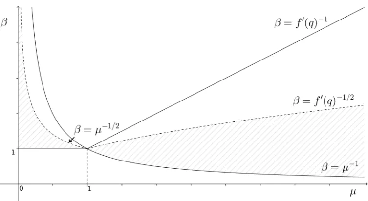
Figure 1.3 is the phase diagram indicating the regimes in which the walk can

obey a central limit theorem. Whether or not the walk does obey a central limit theorem depends on the moments of the offspring distribution; however; our results

show that if the offspring law has finite third moments or exponential moments in

the subcritical and supercritical cases respectively then the walk obeys an annealed functional central limit theorem for the entirety of the region.

(26)

[image:26.595.138.515.84.290.2]

Figure 1.3: Phase diagram with the shaded region indicating the combinations of µ and β

such that the walk obeys a central limit theorem.

consider a related process in Chapter 5. In this chapter we study the randomly trapped

random walk when the holding times have finite mean and infinite variance and show conditions under which the centred and rescaled walk converges to a stable process.

We apply this result to the comb model which can be seen as the subcritical

GW-tree model where each branch is pruned so that it consists only of the unique path to the deepest vertex. As in the sub-ballistic regime, we expect that this structure

should determine the correct scaling of the walk on the subcritical tree; in particular, it

suggests that|Xn−nνβ| 'n1/γ. Similarly to the sub-ballistic regime for the subcritical

GW-tree, we only observe convergence along certain subsequences in the comb model

(27)

Chapter 2 Preliminaries

In this chapter we provide the necessary background and several technical results that we use throughout the thesis. We do not prove any new results in Section 2.1 but give

a brief overview of Skorohod topologies which will play an important role in much of

the thesis. In Section 2.2 we state some well known formulas concerning stable laws and prove a straightforward technical lemma. We cover basic estimates relating to

random walks in Section 2.3. This includes the classical Gambler’s ruin, expressions

for expected cover times and an upper bound on the correlation between the number of visits to two vertices in a tree. In Section 2.4 we address branching processes by stating

some classical formulas and proving two technical results which we use throughout.

We conclude the chapter in Section 2.5 by proving that we can couple a random walk on a subcritical GW-tree conditioned to survive with a randomly trapped random

walk so that the two walks do not deviate too far from each other.

2.1 Skorohod topologies

In this section we briefly outline the space of c`adl`ag functions, the Skorohod J1, M1

andM2 topologies and several useful results that we apply throughout the thesis.

Ev-erything stated here can be found in [76] to which we direct the reader for more detail.

We also refer the reader to [18] and [45] which give a good account of convergence of

stochastic processes in this setting.

In short, the space of continuous functions is not a suitable choice to describe

many of the processes we consider which must contain jumps. We, therefore, consider

instead the space of c`adl`ag functionsD([0, T],R) mapping [0, T] ontoR; that is, those functions which are right continuous and have left limits.

Because we consider processes with discontinuous paths, the uniform topology

will not always be an appropriate choice. We consider, instead, the Skorohod topolo-gies which consider functions to be close if they can be mapped onto one another by a

(28)

perturbations in space reflected by the uniform topology.

Let Λ be the set of strictly increasing continuous functions mapping [0, T] onto itself. We then consider the SkorohodJ1 metric dJ1 on D([0, T],R) defined by

dJ1(f, g) := inf

λ∈Λ_t_∈sup_[0_,T_](|f(t)−g(λ(t))|+|t−λ(t)|). (2.1)

For f ∈ D([0, T],R) let Γf := {(z, t) ∈ R ×[0, T] : z = αf(t−) + (1− α)f(t) for someα ∈ [0,1]} be the completed graph of f. We then define an or-dering on Γf by saying that (z1, t1) ≤ (z2, t2) if either t1 < t2 or t1 = t2 and

|f(t−₁)−z1| ≤ |f(t−2)−z2|. A parametric representation of Γf is a non-decreasing

functionu = (u1, u2) : [0, T]→ Γf. Let Πf denote the parametric representations of

Γf then we define the Skorohod M1 metric dM1 on D([0, T],R) as

dM1(f, g) := inf

u∈Πf,v∈Πg

(|u1−v1| ∨ |u2−v2|).

This is weaker than theJ1 topology; in particular, it allows a discontinuous jump and

a continuous surge to be close which theJ1 topology does not.

Finally, we define the SkorohodM2 distance by

dM2(f, g) := sup

(zf,tf)∈Γf

inf

(zg,tg)∈Γg

(|zf −zg| ∨ |tf −tg|)

∨ sup

(zg,tg)∈Γg

inf

(zf,tf)∈Γf

(|zf −zg| ∨ |tf −tg|).

This is weaker than the M1 topology since it only requires that all points on the

completed graph off are close to some other point on the completed graph ofg. We extend this notion to D:= D([0,∞),R) by characterising convergence in the respective topologies. We say thatfn →f inD([0,∞),R) with the Skorohod J1

(orM1, M2) topology if and only iffn→f in inD([0, T],R) with the SkorohodJ1 (or

M1, M2) topology for every continuity pointT off. Furthermore, for convenience, we

will often writeDJ1([0,∞),R) to denoteD([0,∞),R) equipped with the Skorohod J1

topology and likewise withU,M1 orM2.

We now state [76, Theorems 13.2.1, 13.2.2, 13.6.3, 13.7.1 & Corollary 13.6.4]

which will be used throughout the thesis. We writeD↑, D↑↑to denote the subsets ofD

which are increasing and strictly increasing respectively. We then writeDu, Du,↑, Du↑↑ for those subsets of unbounded functions. Furthermore, C, C↑, C↑↑ denote the

corre-sponding subsets of continuous functions.

(29)

to D is measurable and continuous at(f, g)∈C×C↑;

ii) (J1-continuity of composition) The composition map from D×D↑ to D taking

(f, g) into (f ◦g) is continuous at (f, g) ∈ (C ×D↑)∪(D×C↑↑) using the J1 topology throughout;

iii) (equivalent characterisations of convergence for monotone functions) Suppose that

(fn)n≥1, f ∈Du,↑, then the following are equivalent:

(a) fn→f in Du↑ with theM1 topology;

(b) fn→f for allt in a dense subset of (0,∞);

(c) f_n−1→f−1 in Du↑ with the M1 topology;

(d) f_n−1→f−1 for allt in a dense subset of (0,∞);

iv) (inverse with linear centring) Supposecn(fn−e)→f as n→ ∞ in D([0,∞),R)

with one of the topologies M2, M1 or J1 where fn∈ Du, cn→ ∞, f(0) = 0 and

e denotes the identity map.

(a) If the topology is M2 or M1, then cn(fn−1 −e) → −f as n → ∞ with the

same topology.

(b) If the topology is J1 and f has no positive jumps, then cn(fn−1−e)→ −f as

n→ ∞ with theJ1 topology.

v) (continuity of the inverse at strictly increasing functions) The inverse map from

(Du, M2) to(Du↑, U) is measurable and continuous at f ∈Du↑↑.

2.2 Stable laws

Throughout the thesis we will use a range of properties about stable laws and their domains of attraction. We state them here along with several new results that will be

useful later. For a more detailed introduction and proofs of some of these facts, we

direct the reader to [15] and [34].

We begin with a note concerning slowly and regularly varying functions. We

say that a functionL varies slowly (at∞) if for anyc >0 we have that

lim

x→∞ L(cx)

L(x) = 1

and that the functionRvaries regularly (with indexα) if there exists a slowly varying functionLsuch that R(x) =xα_L(x).

For the purposes of this section letξ,{ξk}k≥1 be i.i.d. with law F and define

(30)

bn such that Sn

d

= anξ +bn and F is not concentrated at a single point. By [34,

Theorem VI.1.1] we have that an = n1/α for some α ∈ (0,2]. We refer to α as the

index ofF.

We say thatF belongs to the domain of attraction of a distributionG if there exist constants an > 0, bn such that an−1(Sn−bn) converges in distribution to G as

n → ∞. This is clearly true for F if it is a stable distribution therefore any stable

distribution posses a domain of attraction. In fact, a distribution is stable if and only if it possesses a domain of attraction. A useful result of [34, Chapter XVII.5] is that

ifF belongs to the domain of attraction of a stable law with index α <2 thenξ has

finite absolute moments for allβ < α and no moments of order β > α exist.

For much of the thesis we will consider only positive random variables so

sup-pose ξ is almost surely positive. Forζ, η >0 let

Uζ(x) :=E

h

ξζ1{ξ≤x}

i

and Vη(x) :=Eξη1{ξ≥x}

denote the truncated moment functions ofξ. By [34, Theorem IX.8.1], F belongs to

the domain of attraction of a stable law with indexα∈(0,2] if and only if there exists a slowly varying functionLsuch that, asx→ ∞,

U2(x)∼x2−αL(x). (2.2)

Moreover, (2.2) is fully equivalent to

P(ξ ≥x)∼ 2 −α

α x

−α_L(x) _(2.3)

whenα <2 therefore we will often consider this relation instead.

Suppose that limx→∞Uζ(x) =∞; then, if eitherUζorVη varies regularly then,

by [34, Theorem VIII.9.2] there exists a limit

lim

x→∞ xζ−η_V

η(x)

Uζ(x)

=c (2.4)

wherecmay be 0 or∞; however,c∈ {0,∞}can only be the case whenUζorVη varies

slowly.

This concludes the basic theory of stable laws that we require for the thesis. We now include two technical results which will be used later. Lemma 2.2.1 shows that

the product of an exponential random variable with a heavy tailed random variable

has a similar tail to the heavy tailed variable.

Lemma 2.2.1. Let X ∼exp(θ) for θ > 0 and suppose ξ is an independent, positive random variable which belongs to the domain of attraction of a stable law of index

(31)

Proof. For some slowly varying function L we have that P(ξ ≥ x) ∼ x−αL(x) as x→ ∞.

Fix 0< u <1< v <∞then ∀y≤u we have thatx/y > x thusP(ξ ≥x/y)≤

P(ξ≥x) it therefore follows that

0≤

Z u 0

θe−θyP(ξ ≥x/y)

P(ξ≥x) dy ≤

Z u 0

θe−θydy= 1−eθu. We have thatP(ξ ≥x/y)/P(ξ≥x)→yα uniformly overy ∈[u, v] therefore

lim

x→∞

Z v

u

P(ξ≥x) dy=

Z v

u

θe−θyyαdy.

Moreover, since this holds for allu≥0 and 1−eθu→0 as u→0 we have that lim

x→∞

Z v 0

P(ξ≥x) dy=

Z v 0

θe−θyyαdy. (2.5) Since 0 <P(ξ ≥ x) ≤1 for all x <∞ we have that L is bounded away from {0,∞} on any compact interval thus satisfies the requirements of Potter’s theorem

(see, for example, [19, Section 1.5.4]) that if L is slowly varying and bounded away

from {0,∞} on any compact subset of [0,∞) then for any > 0 there exists A > 1

such that forx, y >0

L(z)

L(x) ≤Amax

nz

x

,x z

o

.

Moreover,∃c1, c2 >0 such thatc1t−αL(t)≤P(ξ≥t)≤c2t−αL(t) hence we have that

for ally > v P(ξ ≥x/y)/P(ξ≥x)≤Cyα+. By dominated convergence we therefore have that

lim

x→∞

Z ∞

v

P(ξ≥x) dy=

Z ∞

v

θe−θyyαdy. Combining this with (2.5) we have that

lim

x→∞

P(Xξ≥x)

P(ξ ≥x) = limx→∞

Z ∞

0

P(ξ ≥x) dy=

Z ∞

0

θe−θyyαdy=θ−αΓ(α+ 1).

The following lemma concerning the form of the probability generating function of the offspring distribution will be fundamental in determining the distribution over

the number of large traps rooted at a given backbone vertex in Chapter 4. The case

µ = 1 appears in [20]; the proof of Lemma 2.2.2 is a simple extension therefore we omit it.

(32)

1. If µ≤1 then as s→1−

E[sξ]−sµ∼ Γ(3−α)

α(α−1)(1−s)

α_L((1₋_s)−1₎ where Γ(t) =R∞

0 xt

−1_e−x_dx _{is the usual gamma function.}

2. If µ >1 then

1−E[sξ] =µ(1−s) +Γ(3−α)

α(α−1)(1−s)

α_L((1₋_s)−1₎

where L varies slowly at∞.

2.3 Random walks and random variables

We now state several classical results for random variables which will be used through-out the thesis. Suppose thatSn is the partial sum of a sequence of independent,

cen-tred random variablesXk andλ >0, then Kolmogorov’s maximal inequality (e.g. [17])

states that

P

max

1≤k≤n|Sk| ≥λ

≤λ−2

n

X

k=1

Var(Xk).

A similar result that we will use later is Doob’s inequality (e.g. [33]) which states that ifMn is a submartingale then

P

max

1≤k≤nMk≥λ

≤λ−1E

h

Mn1{max1≤k≤nMk≥λ}

i

≤λ−1E[Mn∨0].

Another related result is the Lp maximal inequality (e.g. [33]) which states that for Mn a submartingale and 1< p <∞ we have that

E

max

1≤k≤nM p k

≤

p p−1

p

EMnp1{Mn≥0}

.

Binomial random variables will play a key role in the decomposition of excursion times in trees. Suppose thatB is binomially distributed with ntrials of success probability

p∈(0,1). Letµ=npbe the expected number of successes then the Chernoff bounds

(e.g. [60]) state that forδ∈(0,1) we have that

P(B ≥(1 +δ)µ)≤e−

δ2µ

3 and _P(B ≤(1−δ)µ)≤e−

δ2µ

2 .

For much of the thesis we will be concerned with invariance principles. To this end, we will often apply the quintessential Donsker’s invariance principle (e.g. [32],

(33)

variablesXk with mean 0 and variance 1 thenSbntcn−1/2 converges in distribution on DJ1([0,∞),R) to a standard Brownian motion.

A useful technique for deriving limiting results is to exploit ergodicity. We will

benefit from Birkhoff’s ergodic theorem (e.g. [16], [48]) which gives us that if ξ is a

random variable with law P in a space Ω and θ is an ergodic P-preserving transfor-mation on Ω then, for any measurable functionf ≥0, we have thatn−1Pn−1

k=0f(θkξ)

converges toE[f(ξ)] as n→ ∞ forP-a.e.ξ.

The following result is [10, Theorem 10.2], and is itself a consequence of [66, Theorem IV.6]. This gives a set of necessary and sufficient conditions for a random

i.i.d. sum to converge to a certain infinitely divisible law.

Proposition 2.3.1. Let n(t) : [0,∞)→_Nand for each tlet{Rk(t)} n(t)

k=1 be a sequence of i.i.d. random variables. Assume that for every >0 it is true that

lim

t→∞P(R1(t)> ) = 0.

Now, suppose L(x) : R \ {0} → R is a real, non-decreasing function satisfying limx→∞L(x) = 0 and R₀ax2dL(x) < ∞ for all a > 0. Let d ∈ R and ς ≥ 0,

then the following statements are equivalent:

1. As t→ ∞

n(t) X

k=1

Rk(t)

d

→Rd,ς,L

where Rd,ς,L has the lawI(d, ς,L), that is,

E[eitRd,ς,L] := exp

idt−ς

2_t2

2 +

Z ∞

−∞

eitx−1− itx 1 +x2

dL(x)

. (2.6)

2. For τ >0 let Rτ(t) :=R1(t)1{|R1(t)|≤τ} then for every continuity point x of L

d= lim

t→∞n(t)E[Rτ(t)] +

Z

|x|>τ

x

1 +x2dL(x)− Z

0<|x|≤τ

x3

1 +x2dL(x),

ς2 = lim

τ→0lim supt→∞

n(t)Var(Rτ(t)),

L(x) =







limt→∞n(t)P(R1(t)≤x) x <0

−limt→∞n(t)P(R1(t)> x) x >0

A fundamental aspect of the random walk on GW-tree model is the concept of trapping. For this reason it will be extremely important to understand the time spent