Bayesian Quadratic Discriminant Analysis
Santosh Srivastava [email protected]
Department of Applied Mathematics University of Washington
Seattle, WA 98195, USA
Maya R. Gupta [email protected]
Department of Electrical Engineering University of Washington
Seattle, WA 98195, USA
B´ela A. Frigyik [email protected]
Department of Mathematics Purdue University
West Lafayette, IN 47907, USA
Editor: Saharon Rosset
Abstract
Quadratic discriminant analysis is a common tool for classification, but estimation of the Gaus-sian parameters can be ill-posed. This paper contains theoretical and algorithmic contributions to Bayesian estimation for quadratic discriminant analysis. A distribution-based Bayesian classifier is derived using information geometry. Using a calculus of variations approach to define a functional Bregman divergence for distributions, it is shown that the Bayesian distribution-based classifier that minimizes the expected Bregman divergence of each class conditional distribution also minimizes the expected misclassification cost. A series approximation is used to relate regularized discrimi-nant analysis to Bayesian discrimidiscrimi-nant analysis. A new Bayesian quadratic discrimidiscrimi-nant analysis classifier is proposed where the prior is defined using a coarse estimate of the covariance based on the training data; this classifier is termed BDA7. Results on benchmark data sets and simulations show that BDA7 performance is competitive with, and in some cases significantly better than, reg-ularized quadratic discriminant analysis and the cross-validated Bayesian quadratic discriminant analysis classifier Quadratic Bayes.
Keywords: quadratic discriminant analysis, regularized quadratic discriminant analysis, Bregman
divergence, data-dependent prior, eigenvalue decomposition, Wishart, functional analysis
1. Introduction
One approach to resolve the ill-posed estimation is to regularize the covariance estimation; another approach is to use Bayesian estimation.
Bayesian estimation for QDA was first proposed by Geisser (1964), but this approach has not become popular, even though it minimizes the expected misclassification cost. Ripley (2001) in his text on pattern recognition states that such predictive classifiers are mostly unmentioned in other texts and that “this may well be because it usually makes little difference with the tightly constrained parametric families.” Geisser (1993) examines Bayesian QDA in detail, but does not show that in practice it can yield better performance than regularized QDA. In preliminary experiments we found that the performance of Bayesian QDA classifiers is very sensitive to the choice of prior (Srivastava and Gupta, 2006), and that priors suggested by Geisser (1964) and Keehn (1965) produce error rates similar to those yielded by ML.
In this paper we propose a Bayesian QDA classifier termed BDA7. BDA7 is competitive with regularized QDA, and in fact performs better than regularized QDA in many of the experiments with real data sets. BDA7 differs from previous Bayesian QDA methods in that the prior is selected by crossvalidation from a set of data-dependent priors. Each data-dependent prior captures some coarse information from the training data. Using ten benchmark data sets and ten simulations, the performance of BDA7 is compared to that of Friedman’s regularized quadratic discriminant analysis (RDA) (Friedman, 1989), to a model-selection discriminant analysis (EDDA) (Bensmail and Celeux, 1996), to a modern cross-validated Bayesian QDA (QB) (Brown et al., 1999), and to ML-estimated QDA, LDA, and the nearest-means classifier. Our focus is on cases in which the number of dimensions d is large compared to the number of training samples n. The results show that BDA7 performs slightly better than the other approaches averaged over the real data sets. The simulations help analyze the methods under controlled conditions.
This paper also contributes to the theory of Bayesian QDA in several aspects. First, the Bayesian classifier is solved for in terms of the Gaussian distributions themselves, as opposed to the standard approach of formulating the problem in terms of the Gaussian parameters. This distribution-based Bayesian discriminant analysis removes the parameter-based Bayesian analysis restriction of re-quiring more training samples than feature dimensions, and removes the question of invariance to transformations of the parameters, because the estimate is defined in terms of the Gaussian dis-tribution itself. We show that the disdis-tribution-based Bayesian discriminant analysis classifier has roughly the same closed-form as the parameter-based Bayesian discriminant analysis classifier, but has a different degree of freedom.
The second theoretical result links Bayesian QDA and Friedman’s regularized QDA by a using series approximation. Third, we show that the Bayesian distribution-based classifier that minimizes the expected misclassification cost is equivalent to the classifier that uses the Bayesian minimum expected Bregman divergence estimates of the class conditional distributions.
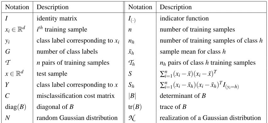
Notation Description Notation Description
I identity matrix I(·) indicator function
xi∈Rd ithtraining sample n number of training samples
yi class label corresponding to xi nh number of training samples of class h
G number of class labels x¯h sample mean for class h
T
n pairs of training samplesT
h nhpairs of class h training samplesx∈Rd test sample S ∑n
i=1(xi−x¯)(xi−x¯)T
Y class label corresponding to x Sh ∑ni=1(xi−x¯h)(xi−x¯h)TI(yi=h)
C misclassification cost matrix |B| determinant of B
diag(B) diagonal of B tr(B) trace of B
N random Gaussian distribution
N
realization of a Gaussian distributionTable 1: Key Notation
classifiers, followed by further analysis using simulation results in Section 8. The paper concludes with a discussion of the results and some open questions.
Table 1 details some of the notation used in this paper.
2. Prior Research on Ill-Posed QDA
We review the prior literature on Bayesian approaches to QDA, regularization approaches to QDA, and other approaches to resolving ill-posed QDA.
2.1 Bayesian Approaches to QDA
Discriminant analysis using Bayesian estimation was first proposed by Geisser (1964) and Keehn (1965). Geisser’s work used a noninformative prior distribution to calculate the posterior odds that a test sample belongs to a particular class. Keehn’s work assumed that the prior distribution of the covariance matrix is an inverse Wishart distribution. Raudys and Jain (1991) stated that Bayesian QDA does not solve the problems that occur with ML QDA, particularly when class sample sizes differ. Recent work by the authors showed that Bayesian QDA using the priors suggested by Geisser and Keehn perform similarly to ML QDA on six standard QDA simulations (Srivastava and Gupta, 2006).
The inverse Wishart prior is a conjugate prior for the covariance matrix, and it requires the specification of a “seed” positive definite matrix and a scalar degree of freedom. Following Brown et al. (1999), the term Quadratic Bayes (QB) is used to refer to a modern form of Bayesian QDA where the inverse Wishart seed matrix is kI, where I is the d-dimensional identity matrix, k is a scalar, and the parameters k and the degree of freedom q of the inverse Wishart distribution are chosen by crossvalidation.
calculated with respect to Lebesgue measure over the domain of the parameters. In this paper we solve for the distribution-based Bayesian QDA, such that the uncertainty is considered to be over the set of Gaussian distributions and the Bayesian estimation is formulated over the domain of the Gaussian distributions.
2.2 Regularizing QDA
Friedman (1989) proposed regularizing ML covariance estimation by linearly combining a ML estimate of each class covariance matrix with the ML pooled covariance estimate and with a scaled version of the identity matrix to form an estimate ˆΣh(λ,γ)for the hth class:
ˆ
Σh(λ) =
(1−λ)Sh+λS
(1−λ)nh+λn
, (1)
ˆ
Σh(λ,γ) = (1−γ)Σˆh(λ) +
γ
dtr ˆΣh(λ)
I. (2)
The above notation and other key notation is defined in Table 1.
In Friedman’s regularized QDA (RDA), the parameters λ,γ are trained by crossvalidation to be those parameters that minimize the number of classification errors. Friedman’s comparisons to ML QDA and ML linear discriminant analysis on six simulations showed that RDA could deal effectively with ill-posed covariance estimation when the true covariance matrix is diagonal. RDA is perhaps the most popular approach to discriminant analysis when the covariance estimation is expected to be ill-posed (Hastie et al., 2001).
Hoffbeck and Landgrebe (1996) proposed a similar regularized covariance estimate for classifi-cation of the form
ˆ
Σ=α1diag(ΣˆML) +α2ΣˆML+α3Σˆpooled ML+α4diag(Σˆpooled ML),
where ˆΣMLand ˆΣpooled MLare maximum likelihood estimates of class and pooled covariance matri-ces, respectively, and the parametersα1,α2,α3,α4 are trained by crossvalidation to maximize the likelihood (whereas Friedman’s RDA crossvalidates to maximize classification accuracy). Results on Friedman’s simulation suite and experimental results on a hyperspectral classification problem showed that the two classifiers achieved similar accuracy (Hoffbeck and Landgrebe, 1996). An-other restricted model used to regularize covariance matrix estimation is a banded covariance matrix (Bickel and Li, 2006).
RDA and the Hoffbeck-Landgrebe classifiers linearly combine different covariance estimates. A related approach is to select the best covariance model out of a set of models using crossvalidation. Bensmail and Celeux (1996) propose eigenvalue decomposition discriminant analysis (EDDA), in which fourteen different models for the class covariances are considered, ranging from a scalar times the identity matrix to a full class covariance estimate for each class. The model that minimizes the crossvalidation error is selected for use with the test data. Each individual model’s parameters are estimated by ML; some of these estimates require iterative procedures that are computationally intensive.
2.3 Other Approaches to Quadratic Discriminant Analysis
Other approaches have been developed for ill-posed quadratic discriminant analysis. Friedman (1989) notes that, beginning with work by James and Stein in 1961, researchers have attempted to improve the eigenvalues of the sample covariance matrix. Another approach is to reduce the data dimensionality before estimating the Gaussian distributions, for example by principal components analysis (Swets and Weng, 1996). One of the most recent algorithms of this type is orthogonal linear discriminant analysis (Ye, 2005), which was shown by the author of that work to perform similarly to Friedman’s regularized linear discriminant analysis on six real data sets.
3. Distribution-based Bayesian Discriminant Analysis
Parameter estimation depends on the form of the parameter, for example, Bayesian estimation can yield one result if the expected standard deviation is solved for, or another result if the expected variance is solved for. To avoid this issue we derive Bayesian QDA by formulating the problem in terms of the Gaussian distributions explicitly. This section extends work presented in a recent conference paper (Srivastava and Gupta, 2006).
Suppose one is given an iid training set
T
={(xi,yi),i=1,2, . . .n}and a test sample x, wherexi,x∈Rd, and yi takes values from a finite set of class labels yi ∈ {1,2, . . . ,G}. Let C be the misclassification cost matrix such that C(g,h)is the cost of classifying x as class g when the truth is class h. Let P(Y =h) be the prior probability of class h. Suppose the true class conditional distributions p(x|Y =h) exist and are known for all h, then the estimated class label for x that minimizes the expected misclassification cost is
Y∗ 4=argmin g=1,...,G
G
∑
h=1
C(g,h)p(x|Y=h)P(Y =h). (3)
In practice the class conditional distributions and the class priors are usually unknown. We model each unknown distribution p(x|h)by a random Gaussian distribution Nh, and we model the unknown class priors by the random vectorΘ, which has componentsΘh=P(Y=h)for h=1, . . . ,G. Then, we estimate the class label that minimizes the expected misclassification cost, where the expecta-tion is with respect to the random distribuexpecta-tions Θ and{Nh}for h=1, . . . ,G. That is, define the
distribution-based Bayesian QDA class estimate by replacing the unknown distributions in (3) with their random counterparts and taking the expectation:
ˆ
Y =4 argmin g=1,...,G
E
"
G
∑
h=1
C(g,h)Nh(x)Θh
#
. (4)
In (4) the expectation is with respect to the joint distribution overΘand{Nh}for h=1, . . . ,G, and these distributions are assumed independent. Therefore (4) can be rewritten as
ˆ
Y =argmin g=1,...,G
G
∑
h=1
C(g,h)ENh[Nh(x)]EΘ[Θh]. (5)
Straightforward integration yields an estimate of the class prior, EΘ[Θh] = nnh++1G; this Bayesian esti-mate for the multinomial is also known as Laplace correction (Jaynes and Bretthorst, 2003).
3.1 Statistical Models and Measure
Consider the family M of multivariate Gaussian probability distributions onRd. Let each element
of M be a probability distribution
N
:Rd→[0,1], parameterized by the real-valued variables(µ,Σ)in some open set inRd⊗S, whereS⊂Rd(d+1)/2 is the cone of positive semi-definite symmetric matrices. That is M ={
N
(·; µ,Σ)} defines a d2+3d2 -dimensional statistical model, (Amari and Nagaoka, 2000, pp. 25–28).Let the differential element over the set M be defined by the Riemannian metric (Kass, 1989; Amari and Nagaoka, 2000),
dM = |IF(µ,Σ)|
1
2dµdΣ, where
IF(µ,Σ) = −EX[∇2log
N
(X ;(µ,Σ))],where∇2is the Hessian operator with respect to the parameters µ andΣ, and this IF is also known as the Fisher information matrix. Straightforward calculation shows that
dM = dµ
|Σ|12
dΣ
|Σ|d+21
= dµdΣ
|Σ|d+22
. (6)
Let
N
h(µh,Σh)be a possible realization of the Gaussian pdf Nh. Using the measure defined in (6),ENh[Nh(x)] = Z
M
N
h(x)r(
N
h)dM, (7)where r(
N
h)is the posterior probability ofN
hgiven the set of class h training samplesT
h; that is,r(
N
h) =`(
N
h,T
h)p(N
h)αh
, (8)
whereαhis a normalization constant, p(
N
h)is the prior probability ofN
h(treated further in Section 3.2), and`(N
h,T
h)is the likelihood of the dataT
hgivenN
h, that is,`(
N
h(µh,Σh),T
h) =exp[−12tr Σ−h1Sh
−nh
2 tr Σ− 1
h (µh−X¯h)(µh−X¯h)T
]
(2π)dnh2 |Σh|nh2
. (9)
3.2 Priors
A prior probability distribution of the Gaussians, p(
N
h), is needed to solve the classification prob-lem given in (4). A common interpretation of Bayesian analysis is that the prior represents informa-tion that one has prior to seeing the data (Jaynes and Bretthorst, 2003). In the practice of statistical learning, one often has very little quantifiable information apart from the data. Instead of thinking of the prior as representing prior information, we considered the following design goals: the prior should• regularize the classification to reduce estimation variance, particularly when the number of training samples n is small compared to the number of feature dimensions;
• allow the estimation to converge to the true generating class conditional normals as n→∞if in fact the data was generated by class conditional normals;
• lead to a closed-form result.
To meet these goals, we use as a prior
p(
N
h) =p(µh)p(Σh) =γ0exp[−12tr Σ−h1Bh
]
|Σh|
q
2
, (10)
where Bh is a positive definite matrix (further specified in (25)) andγ0is a normalization constant. The prior (10) is equivalent to a noninformative prior for the mean µ, and an inverted Wishart prior with q degrees of freedom overΣ.
This prior is unimodal and leads to a closed-form result. Depending on the choice of Bhand q, the prior probability mass can be focused over a small region of the set of Gaussian distributions M in order to regularize the estimation. Regularization is important for cases where the number of training samples n is small compared to the dimensionality d. However, the tails of this prior are sufficiently heavy that the prior does not hinder convergence to the true generating distribution as the number of training samples increases if the true generating distribution is normal.
The positive definite matrix Bh specifies the location of the maximum of the prior probability distribution. Using the matrix derivative (Dwyer, 1967) and the knowledge that the inverse Wishart distribution has only one maximum, one can calculate the location of the maximum of the prior. Take the log of the prior,
log p(
N
h) =− 1 2tr Σ−1 h Bh
−q
2log|Σh|+logγ0. Differentiate with respect toΣhto solve forΣh,max,
−12∂Σ∂ h
tr
Σ−1
h,maxBh
−q2∂Σ∂
h
log|Σh,max| = 0,
Σ−1
h,maxBhΣ−h,max1 −qΣ−h,max1 = 0,
Σh,max = Bh
q . (11)
Because this prior is unimodal, a rough interpretation of its action is that it regularizes the likelihood covariance estimate towards the maximum of the prior, given in (11). To meet the goal of minimizing bias, we encode some coarse information about the data into Bh. In QB (Brown et al., 1999), the prior seed matrix Bh=kI, where k is a scalar determined by crossvalidation. Setting
Bh =kI is reminiscent of Friedman’s RDA (Friedman, 1989), where the covariance estimate is
regularized by the trace: tr(ΣˆdML)I.
We have shown in earlier work that setting Bh= tr(ΣˆML)
priors, including hyperparameters and empirical Bayes methods (Efron and Morris, 1976; Haff, 1980; Lehmann and Casella, 1998). Data-dependent priors are also used to form proper priors that act similarly to improper priors, or to match frequentist goals (Wasserman, 2000). Next, we describe the closed form result with a prior of the form given in (10), then we return to the question of data-dependent definitions for Bhwhen we propose the BDA7 classifier in Section 6.
3.3 Closed-Form Result
In Theorem 1 we establish the closed-form result for the distribution-based Bayesian QDA classi-fier. The closed-form result for the parameter-based classifier with the same prior is presented after the theorem for comparison.
Theorem 1: The classifier (5) using the prior (10) can be written as
ˆ
Y =argmin g=1,...,G
G
∑
h=1 C(g,h)
(nh)
d
2Γ
nh+q+1
2
Sh+Bh 2
nh+q
2
(nh+1)
d
2Γ
nh+q−d+1 2
|Ah|
nh+q+1 2
ˆ
P(Y =h), (12)
where ˆP(Y =h)is an estimate of the class prior probability for class h,Γ(·)is the standard gamma function, and
Ah= 1 2
Sh+
nh(x−x¯h)(x−x¯h)T
(nh+1)
+Bh
. (13)
The proof of the theorem is given in Appendix A. The parameter-based Bayesian QDA class label using the prior given in (10) is
ˆ
Y =argmin g=1,...,G
G
∑
h=1 C(g,h)
(nh)
d
2Γ
nh+q−d−1 2
(nh+1)
d
2Γ
nh+q−2d−1 2
|Sh+Bh
2 | nh+q−d−2
2
|Ah|
nh+q−d−1 2
ˆ
P(Y=h). (14)
Equation (14) can be proved by following the same steps as the proof of Theorem 1. The parameter-based Bayesian discriminant result (14) will not hold if nh≤2d−q+1, while the distribution-based result (12) holds for any nh>0 and any d.
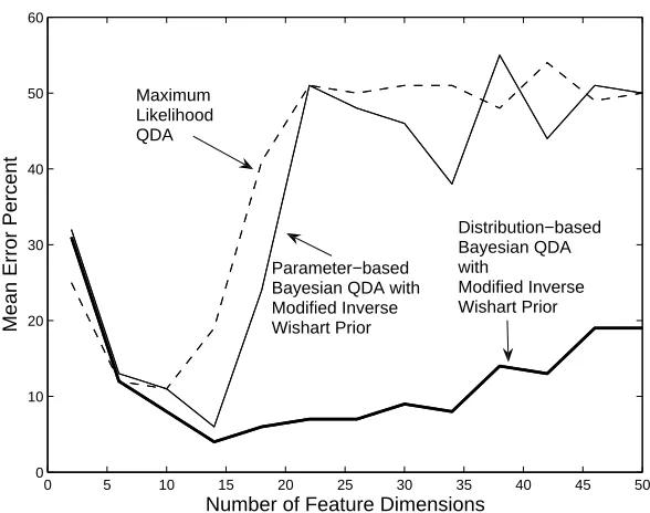
In a previous publication (Srivastava and Gupta, 2006), we compared the distribution-based Bayesian QDA to the parameter-based Bayesian QDA classifier, maximum likelihood QDA, and nearest means. We compared the noninformative prior originally proposed by Geisser (1964), and the modified inverse Wishart prior given in Equation (10) with Bh=tr ˆΣML,h/d
I. We fixed the degrees of freedom for the modified inverse Wishart to be d+3, so that in one-dimension it reduces to the common inverted gamma distribution. Results on six simulations (two-class versions of Friedman’s original simulations) showed that given the same prior, the distribution-based performed better than the parameter-based when the ratio of feature dimensions to number of training samples is high. For the reader’s convenience, we include a representative set of the simulation results from Srivastava and Gupta (2006) in Figure 1.
0 5 10 15 20 25 30 35 40 45 50 0
10 20 30 40 50 60
Number of Feature Dimensions
Mean Error Percent
Maximum Likelihood QDA
Parameter−based Bayesian QDA with Modified Inverse Wishart Prior
Distribution−based Bayesian QDA with
Modified Inverse Wishart Prior
Figure 1: Mean error rates are shown for a two-class simulation where the samples from each class are drawn from a Gaussian distribution with the same mean but different, highly-ellipsoidal covariance matrices. The error rates were averaged over 1000 random trials, where on each trial 40 training samples and 100 test samples were drawn iid.
2.1), chooses the degree of freedom for the modified inverse Wishart prior by cross-validation. If one cross-validates the degree of freedom, then it does not matter if one starts from the parameter-based formula or the distribution-parameter-based formula. In Section 6, we propose a new Bayesian QDA classifier called BDA7 that cross-validates the degree of freedom and a data-dependent seed matrix Bhfor the prior. But first we consider further the analytic properties of Bayesian QDA; in the next section we develop a relationship between regularized QDA and Bayesian QDA, and then in Section 5 we show how Bayesian QDA is the solution to minimizing any expected Bregman divergence.
4. Relationship Between Regularized QDA and Bayesian QDA
Let Dh=Sh+Bh,Zh=x−x¯h. The distribution-based Bayesian discriminant formula for the class conditional pdf (12) can be simplified to
ENh[Nh] =
n d
2
hΓ
nh+q+1 2
(2π)d2(nh+1)
d
2Γ
nh+q−d+1 2 Dh 2
nh+q
2 Dh 2 + nh 2(nh+1)ZhZ
T h
nh+q+1 2 = n d 2 hΓ
nh+q+1 2
D2h
nh+q
2
(2π)d2(nh+1)
d
2Γ
nh+q−d+1 2
D2h
nh+q+1 2
I+ nh
nh+1
ZhZhTD−h1
−nh+2q+1
= Γ
nh+q+1 2
(π)d2
nh+1
nh Dh 1 2
Γnh+q−d+1 2
1+ nh
nh+1
ZhTD−h1Zh
−nh+2q+1
, (15)
where (15) follows by rearranging terms and applying the identity|I+ZhZThD−h1|=1+ZThD−h1Zh (Anderson, 2003).
Approximate nh/(nh+1)≈1 in (15). Recall the series expansion er=1+r+r2/2. . ., so if r is small, 1+r≈er. We apply this approximation to the term 1+ZhTD−h1Zhin (15), and note that the approximation is better the closer the test point x is to the sample mean ¯xh, such that Zhis small. The approximation is also better the larger the minimum eigenvalueλmin of Dh is, because of the bound|ZThD−h1Zh| ≤ kZhk2/λmin. Then (15) becomes
ENh[Nh] ≈
Γ
nh+q+1
2 exp
h
nh
nh+1Z
T hD−h1Zh
i−nh+
q+1 2
(π)d2
nh+1
nh Dh 1 2 Γ
nh+q−d+1 2
,
=
Γnh+q+1 2
exp
−12Z
T h
h
nh+1
nh+q+1
Dh
nh
i−1
Zh
(π)d2
nh+1
nh Dh 1 2
Γnh+q−d+1 2
. (16)
Let
˜
Σh=4
nh+1
nh+q+1
Dh
nh
. (17)
The approximation (16) resembles a Gaussian distribution, where ˜Σhplays the role of the covariance matrix. Rewrite (17),
˜
Σh =
nh+1
nh+q+1
Sh+Bh
nh
= nh+1
nh+q+1
Sh
nh
+ nh+1
nh+q+1
Bh nh =
1− q nh+q+1
Sh
nh
+ 1
nh+q+1
nh+1
nh
Bh. (18)
In (18), make the approximation nh+1
nh
≈1, then multiply and divide the second term of (18) by q,
˜
Σh≈
1− q nh+q+1
Sh nh + q nh+q+1
Bh
The right-hand side of (19) is a convex combination of the sample covariance and the positive defi-nite matrix Bh
q. This is the same general formulation as Friedman’s RDA regularization (Friedman, 1989), re-stated in this paper in Equations (1) and (2). Here, the fraction n q
h+q+1controls the shrink-age of the sample covariance matrix toward the positive definite matrix Bh
q; recall from (11) that Bh
q is the maximum of the prior probability distribution. Equation (19) also gives information about how the Bayesian shrinkage depends on the number of sample points from each class: fewer training samples nh results in greater shrinkage towards the positive definite matrix Bqh. Also, as the degree of freedom q increases, the shrinkage towards Bh
q increases. However, as q increases, the shrinkage target Bh
q moves towards the zero-matrix.
5. Bregman Divergences and Bayesian Quadratic Discriminant Analysis
In (5) we defined the Bayesian QDA class estimate that minimizes the expected misclassification cost. Then assuming a Gaussian class-conditional distribution, the expected class-conditional dis-tribution is given in (12). A different approach to Bayesian estimation would be to estimate the hth conditional distribution to minimize some expected risk. That is, the estimated class-conditional distribution would be
ˆ
fh=argmin f∈A
Z
M
R(
N
h,f)dM, (20)where R(
N
h,f)is the risk of guessing f if the truth isN
h, the set of functionsA
is defined more precisely shortly, and dM is a probability measure on the set of Gaussians, M. Equation (20) is a distribution-based version of the standard parameter Bayesian estimate given in Ch. 4 of Lehmann and Casella (1998); for example, the standard parameter Bayesian estimate of the mean ˆµ∈Rdwould be formulated
ˆµ=argmin
ψ∈Rd Z
R(µ,ψ)dΛ(µ),
whereΛ(µ)is some probability measure.
Given estimates of the class-conditional distributions{fˆh}from (20), one can solve for the class label as
˜
Y∗=argmin g=1,...,G
G
∑
h=1
C(g,h)fˆh(x)Pˆ(Y =h). (21)
In this section we show that the class estimate ˆY from minimizing the expected misclassification cost as defined in (5) is equivalent to the class estimate ˜Y∗from (21) if the risk function in (20) is a (functional) Bregman divergence. This result links minimizing expected misclassification cost and minimizing an expected Bregman divergence.
divergence that acts on pairs of distributions. This allows us to extend the Banerjee et al. result to the Gaussian case and establish the equivalence between minimizing expected misclassification cost and minimizing the expected functional Bregman divergence.
This section makes use of functional analysis and the calculus of variations; the relevant defini-tions and results from these fields are provided for reference in Appendix B.
Letνbe some measure, and define the set of functions
A
pto beA
p=
a :Rd→[0,1]
a∈Lp(ν),a>0, kakLp(ν)=1
.
5.1 Functional Definition of Bregman Divergence
Letφ:
A
p→Rbe a continuous functional. Let δ2φ[f ;·,·], the second variation ofφ, be strongly positive. The functional Bregman divergence dφ:A
p×A
p→[0,∞)is defined asdφ(f,g) =φ[f]−φ[g]−δφ[g; f−g], (22)
whereδφ[g;·]is the Fr´echet derivative or first variation ofφat g.
Different choices of the functionalφwill lead to different Bregman divergences. As an example, we present theφfor squared error.
5.2 Example (Squared error)
Letφ:
A
2→Rbe definedφ[g] =
Z g2dν.
Perturbing g by a sufficiently nice function a (see Appendix B for more details about the perturbation function a) leads to the difference
φ[g+a]−φ[g] =
Z
g2+2ga+a2−g2
dν.
Then, because
kφ[g+a]−φ[g]−R
2gadνkL2(ν)
kakL2(ν)
=
R a2dν
(R
a2dν)12
,
=
Z a2dν
12
tends to zero askakL2(ν)tends to zero, the differential is
δφ[g; a] =
Z
Using (23), the Bregman divergence (22) becomes
dφ(f,g) =
Z
f2dν− Z
g2dν− Z
2g(f−g)dν
=
Z
f2dν− Z
2 f gdν+
Z g2dν
=
Z
(f−g)2dν
= kf−gk2L2(ν),
which is the integrated squared error between two functions f and g in
A
2. 5.3 Minimizing Expected Bregman DivergenceThe functional definition (22) is a generalization of the standard vector Bregman divergence
dφ˜(x,y) =φ˜(x)−φ˜(y)−∇φ˜(y)T(x−y) where x,y∈Rn, and ˜φ:Rn→Ris strictly convex and twice differentiable.
Theorem 2: Letφ:
A
1→R,φ∈C
3, andδ2φ[f ;·,·]be strongly positive. Suppose the function ˆfh minimizes the expected Bregman divergence between a random Gaussian Nh and any probability density function f ∈A
where the expectation is taken with respect to the distribution r(N
h), such thatˆ
fh=argmin f∈A
ENh[dφ(Nh,f)]. (24)
Then ˆfhis given by
ˆ fh=
Z
M
N
hr(
N
h)dM=ENh[Nh(x)].The proof of the theorem is given in Appendix A.
Corollary: The result of (5) is equivalent to the result of (21) where each ˆfhcomes from (24).
The corollary follows directly from Theorem 2 where r(
N
h)is the posterior distribution ofN
h given the training samples.6. The BDA7 Classifier
but is still relatively stable to estimate. The diagonal of ˆΣML has been used to regularize a regular-ized discriminant analysis (Hoffbeck and Landgrebe, 1996) and model-based discriminant analysis (Bensmail and Celeux, 1996).
Note that setting Bh=diag ˆΣML
places the maximum of the prior at 1qdiag ˆΣML
. We hypoth-esize that in some cases it may be more effective to place the maximum of the prior at diag ˆΣML
; that requires setting Bh=q diag ˆΣML
.
We also consider moving the maximum of the prior closer to the zero matrix, effectively turn-ing the prior into an exponential prior rather than a unimodal one. We expect that this will have the rough effect of shrinking the estimate toward zero. Shrinkage towards zero is a successful technique in other estimation scenarios: for example ridge and lasso regression shrink linear regression coef-ficients toward zero (Hastie et al., 2001), and wavelet denoising shrinks wavelet coefcoef-ficients toward zero. To this end, we also consider setting the prior matrix seed to be Bh= 1qdiag ˆΣML
.
These different choices for Bhwill be more or less appropriate depending on the amount of data and the true generating distributions. Thus, for BDA7 the Bh is selected by crossvalidation from seven options:
Bh=
q diag ˆΣ(pooled ML)
,q diag ˆΣ(class ML,h)
, 1
q diag ˆΣ(pooled ML)
, 1
qdiag ˆΣ(class ML,h)
, diag ˆΣ(pooled ML)
,diag ˆΣ(class ML,h)
, 1
qtr(Σˆ(pooled ML))I.
(25)
To summarize: BDA7 uses the result (12) where q is cross-validated, and Bhis cross-validated as per (25).
7. Experiments with Benchmark Data Sets
We compared BDA7 to popular QDA classifiers on ten benchmark data sets from the UCI Machine Learning Repository. In the next section we use simulations to further analyze the behavior of each of the classifiers.
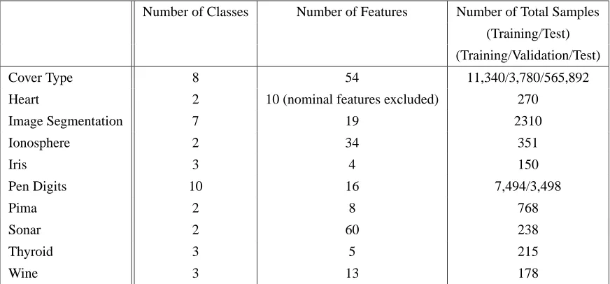
QDA classifiers are best-suited for data sets where there is relatively little data, assuming the class-conditional distribution is Gaussian model can be an appropriate model. For this reason, for data sets with separate training and test sets, Tables 3 and 4 show results on the test set given a randomly chosen 5% or 10% of the training samples. For data sets without separate training and test sets, 5% and 10% of the available samples of each class were randomly selected and used for training, and the rest of the available samples were used as test samples. Each result in Table 3 and 4 is the average test error of 100 trials with different randomly chosen training samples, with the exception of the Cover Type data set, for which only 10 random trials were performed due to its large size. Table 2 summarizes each of the benchmark data sets.
7.1 Experimental Details for Each Classifier
BDA7 is compared with QB (Brown et al., 1999), RDA (Friedman, 1989), eigenvalue decompo-sition discriminant analysis (EDDA) (Bensmail and Celeux, 1996), and maximum-likelihood esti-mated QDA, LDA, and the nearest-means classifier (NM). Code for the classifiers (and the simula-tions presented in the next section) is available at idl.ee.washington.edu.
P(Y =h); those probabilities were estimated based on the number of observations from each class using Bayesian estimation (see Section 3).
The RDA parametersλandγwere calculated and crossvalidated as in Friedman’s paper (Fried-man, 1989) for a total of 25 joint parameter choices.
The BDA7 method is crossvalidated with the seven possible choices of Bhfor the prior specified in (25). The scale parameter q of the inverse Wishart distribution is crossvalidated in steps of the feature space dimension d so that q∈ {d,2d,3d,4d,5d,6d}. Thus there are 42 parameter choices.
The QB method is implemented as described by Brown et al. (1999). QB uses a normal prior for each mean vector, and an inverse Wishart distribution prior for each covariance matrix. There are two free parameters to the inverse Wishart distribution: the scale parameter q≥d and the seed matrix Bh. For QB, Bh is restricted to be spherical: Bh=kI. The parameters q and k are trained by crossvalidation. In an attempt to be similar to the RDA and BDA7 crossvalidations, we allowed there to be 42 parameter choices, q∈ {d,2d,3d,4d,5d,6d}and k∈ {1,2, . . .7}. Other standard Bayesian quadratic discriminant approaches use a uniform (improper) or fixed Wishart prior with a parameter-based classifier (Ripley, 2001; Geisser, 1964; Keehn, 1965); we have previously demonstrated that the inverse Wishart prior performs better than these other choices (Srivastava and Gupta, 2006).
The EDDA method of Bensmail and Celeux is run as proposed in their paper (Bensmail and Celeux, 1996). Thus, the crossvalidation selects one of fourteen models for the covariance, where the ML estimate for each model is used. Unfortunately, we found it computationally infeasible to run the 3rd and 4th model for EDDA for some of the problems. These models are computationally intensive iterative ML procedures that sometimes took prohibitively long for large n, and when n<d these models sometimes caused numerical problems that caused our processor to exit with error. Thus, in cases where the 3rd and 4th model were not feasible, they were not used.
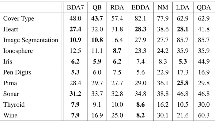
7.2 Results
The results are shown in Tables 3 and 4 for the UCI Machine Learning Repository benchmark data sets described in Table 2. The lowest mean error rate is in bold, as well as any other mean error rate that is not statistically significantly different from the lowest mean error rate, as determined by the Wilcoxon signed rank test for paired-differences at a significance level of.05.
BDA7 was the best or statistically insignificant from the best for seven of the ten tested data sets: Heart, Iris, Image Segmentation, Pen Digits, Sonar, Thyroid, and Wine. For the Pima Dia-betes, Ionosphere, and Cover Type data sets, BDA7 is not the best QDA classifier, but performs competitively.
The Ionosphere data set is a two-class problem with 351 samples described by 34 features. One of the features has the value zero for all samples of class two. This causes numerical difficulties in estimating the maximum likelihood covariance estimates. BDA7 chooses the identity prior seed matrix Bh=1qtr(Σˆ(pooled ML))I every time for this data set. Given that this is BDA7’s choice, BDA7 is at a disadvantage compared to QB, which cross-validates a scaled identity seed matrix kI. In fact, our experiments have showed that shrinking the prior closer to zero improves the performance on this data set, for example using Bh=qd1 tr(Σˆ(pooled ML))I.
Number of Classes Number of Features Number of Total Samples
(Training/Test)
(Training/Validation/Test)
Cover Type 8 54 11,340/3,780/565,892
Heart 2 10 (nominal features excluded) 270
Image Segmentation 7 19 2310
Ionosphere 2 34 351
Iris 3 4 150
Pen Digits 10 16 7,494/3,498
Pima 2 8 768
Sonar 2 60 238
Thyroid 3 5 215
Wine 3 13 178
Table 2: Information About the Benchmark Data Sets
BDA7 QB RDA EDDA NM LDA QDA
Cover Type 48.3 44.6 59.2 83.1 78.5 62.9 62.9
Heart 30.6 38.5 38.2 33.9 39.9 35.9 44.5
Image Segmentation 12.7 12.9 18.3 29.7 29.5 85.7 85.7
Ionosphere 16.9 16.1 12.5 26.0 27.1 35.8 35.8
Iris 6.9 7.6 8.1 9.4 9.3 8.8 66.6
Pen Digits 6.1 8.1 8.5 7.7 23.9 17.8 23.8
Pima 29.7 32.7 29.4 30.7 35.8 27.6 33.4
Sonar 36.8 40.4 40.4 39.8 42.6 46.7 46.7
Thyroid 11.7 14.8 17.0 14.7 19.2 15.0 30.0
Wine 9.6 33.1 34.2 11.2 32.0 60.1 60.1
BDA7 QB RDA EDDA NM LDA QDA
Cover Type 48.0 43.7 57.4 82.1 77.9 62.9 62.9
Heart 27.4 32.0 31.8 28.3 38.6 28.1 41.8
Image Segmentation 10.9 10.8 16.4 27.9 27.7 85.7 85.7
Ionosphere 12.5 11.1 8.7 23.3 24.2 35.9 35.9
Iris 6.2 5.9 6.2 7.4 8.3 5.3 44.9
Pen Digits 5.3 6.0 7.5 5.6 22.9 17.3 16.9
Pima 28.4 29.7 27.7 29.0 36.1 25.8 29.8
Sonar 31.2 33.7 32.8 34.8 38.8 46.8 46.8
Thyroid 7.9 9.1 10.0 8.6 16.2 10.5 30.0
Wine 7.9 16.9 25.0 8.2 30.1 21.6 60.3
Table 4: Average Error Rate Using Randomly Selected 10% of Training Samples
Bh= 1qtr(Σˆ(pooled ML))I. As in the Ionosphere data set, this puts BDA7 at a disadvantage compared to QB, and it is not surprising that on this data set QB does a little better. Despite the numerical difficulties inherent in this problem, the two Bayesian QDA classifiers do better than the other QDA classifiers.
8. Simulations
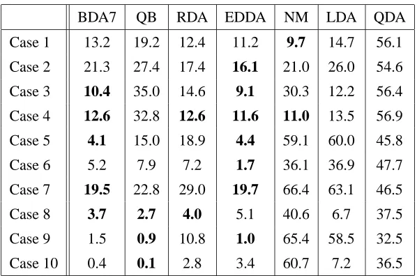
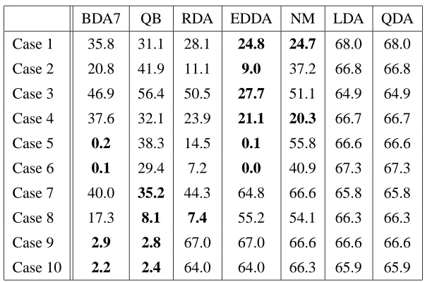
In order to further analyze the behavior of the different QDA classifiers, we compared them in ten simulations. For each of the ten simulations, the data are drawn iid from three Gaussian class con-ditional distributions. Six of the simulations were originally created by Friedman and used to show that RDA performs favorably compared to ML linear discriminant analysis (LDA) and ML QDA (Friedman, 1989). Friedman’s six simulations all have diagonal generating class covariance matri-ces, corresponding to independent classification features. In those cases, the constrained diagonal models used in RDA and EDDA are correct, and so RDA and EDDA’s performance may be opti-mistic compared to real data. For a fuller picture, we add two full covariance matrix simulations to Friedman’s six diagonal Gaussian simulations (Cases 1–6), and for each of the full covariance matrix simulations we consider the cases of classes with the same means (Case 7 and 9), and classes with different means (Case 8 and 10).
All of the simulation results are presented for 40 training and 100 test samples, drawn iid. The parameters for each classifier were estimated by leave-one-out crossvalidation, as described in Section 7.1. Each simulation was run 100 times. Thus, each result presented in Tables 5, 6, and 7 is the average error over 10,000 test samples.
8.1 Simulation Details and Results
diagonal, and are thus a good match to the true generating distributions. When the true generating distributions are drawn from full covariance matrices (Cases 7–10), EDDA performs well when there are only 10 features, but the maximum likelihood estimates used in EDDA fail for 50 and 100 feature dimensions. RDA similarly does well when the true generating distribution matches the RDA models, and like EDDA is unable to learn when the features are highly correlated (Cases 9–10).
BDA7 is rarely the best classifier on the simulations, but never fails to produce relatively rea-sonable error rates. In particular, BDA7 is shown to be a more robust classifier than QB, achieving much lower error rates for Cases 5–6, and lower error rates for Cases 2–4 (with the exception of Case 4 for 100 feature dimensions).
A more detailed analysis and description of each of the simulation cases follows.
8.1.1 CASE1: EQUALSPHERICALCOVARIANCEMATRICES
Each class conditional distribution is normal with identity covariance matrix I. The mean of the first class µ1is the origin, and the second class has zero mean, except that the first component of the second class mean is 3. Similarly, the third class has zero mean, except the last component of the third class mean is 3.
The performance here is bounded by the nearest-means classifier, which is optimal for this simulation. EDDA also does well, because one of the 14 models available for it to choose is exactly correct: scalar times the identity matrix. Similarly, RDA strongly shrinks towards the trace times the identity. Though this is an unrealistic case, it shows that BDA7 can perform relatively well even though it does not explicitly model the true generating distribution.
8.1.2 CASE2: UNEQUALSPHERICALCOVARIANCEMATRICES
The class one conditional distribution is normal with identity covariance matrix I and mean at the origin. The class two conditional distribution is normal with covariance matrix 2I and has zero mean except the first component of its mean is 3. The class three conditional distribution is normal with covariance matrix 3I and has zero mean except the last component of its mean is 4. Like Case 1, EDDA and RDA use the fact that the true generating distributions match their models to outperform BDA7, which is significantly better than QB.
8.1.3 CASES3AND4: EQUALHIGHLYELLIPSOIDAL COVARIANCEMATRICES
Covariance matrices of each class distribution are the same, and highly ellipsoidal. The eigenvalues of the common covariance matrix are given by
ei=
9(i−1)
d−1 +1
2
, 1≤i≤d, (26)
so the ratio of the largest to smallest eigenvalue is 100.
For Case 3 the class means are concentrated in a low-variance subspace. The mean of class one is located at the origin and the ithcomponent of the mean of class two is given by
µ2i=2.5
r
ei
d d−i
BDA7 QB RDA EDDA NM LDA QDA
Case 1 13.2 19.2 12.4 11.2 9.7 14.7 56.1
Case 2 21.3 27.4 17.4 16.1 21.0 26.0 54.6
Case 3 10.4 35.0 14.6 9.1 30.3 12.2 56.4
Case 4 12.6 32.8 12.6 11.6 11.0 13.5 56.9
Case 5 4.1 15.0 18.9 4.4 59.1 60.0 45.8
Case 6 5.2 7.9 7.2 1.7 36.1 36.9 47.7
Case 7 19.5 22.8 29.0 19.7 66.4 63.1 46.5
Case 8 3.7 2.7 4.0 5.1 40.6 6.7 37.5
Case 9 1.5 0.9 10.8 1.0 65.4 58.5 32.5
Case 10 0.4 0.1 2.8 3.4 60.7 7.2 36.5
Table 5: Average Error Rate for 10 Features
BDA7 QB RDA EDDA NM LDA QDA
Case 1 27.9 33.3 25.4 21.7 21.5 67.0 67.0
Case 2 26.8 42.6 15.4 12.5 32.0 66.8 66.8
Case 3 27.2 55.7 44.8 21.2 47.3 66.6 66.6
Case 4 22.5 30.9 17.9 17.0 15.5 67.0 67.0
Case 5 1.2 30.6 11.8 0.0 52.4 66.6 66.6
Case 6 0.5 26.5 8.0 0.0 43.2 66.6 66.6
Case 7 34.7 30.9 41.9 63.9 66.5 66.0 66.0
Case 8 9.2 3.5 2.8 25.5 40.9 66.6 66.6
Case 9 1.3 0.9 62.7 32.5 66.3 66.5 66.5
Case 10 1.7 0.9 60.6 32.4 66.2 66.2 66.2
BDA7 QB RDA EDDA NM LDA QDA
Case 1 35.8 31.1 28.1 24.8 24.7 68.0 68.0
Case 2 20.8 41.9 11.1 9.0 37.2 66.8 66.8
Case 3 46.9 56.4 50.5 27.7 51.1 64.9 64.9
Case 4 37.6 32.1 23.9 21.1 20.3 66.7 66.7
Case 5 0.2 38.3 14.5 0.1 55.8 66.6 66.6
Case 6 0.1 29.4 7.2 0.0 40.9 67.3 67.3
Case 7 40.0 35.2 44.3 64.8 66.6 65.8 65.8
Case 8 17.3 8.1 7.4 55.2 54.1 66.3 66.3
Case 9 2.9 2.8 67.0 67.0 66.6 66.6 66.6
Case 10 2.2 2.4 64.0 64.0 66.3 65.9 65.9
Table 7: Average Error Rate for 100 Features
The mean of class three is the same as the mean of class two except every odd numbered dimension of the mean is multiplied by−1.
Here, BDA7 rivals the performance of EDDA, which makes half the errors of RDA. In contrast, the error rate of QB is twice as high as BDA7 for 10 and 50 dimensions.
Case 4 is that the class means are concentrated in a high-variance subspace. The mean of class one is again located at the origin and the ithcomponent of the mean of class two is given by
µ2i=2.5
r
ei
d i−1
(d2−1), 1≤i≤d.
The mean of class three is the same as the mean of class two except every odd numbered dimension of the mean is multiplied by−1.
8.1.4 CASES5AND6: UNEQUALHIGHLYELLIPSOIDALCOVARIANCEMATRICES
For these cases, the covariance matrices are highly ellipsoidal and different for each class. The eigenvalues of the class one covariance are given by Equation (26), and those of class two are given by
e2i=
9(d−i)
d−1 +1
2
, 1≤i≤d.
The eigenvalues of class three are given by
e3i=
9(i−d−1 2 ) d−1
!2
, 1≤i≤d.
mean of class three is the same as the mean of class two except every odd numbered dimension of the mean is multiplied by−1.
In both these cases the BDA7 error falls to zero as the number of feature dimensions rise, whereas RDA plateaus around 10% error, and QB has substantially higher error. Case 5 and Case 6 present more information to the classifiers than the previous cases because the covariance ma-trices are substantially different. BDA7 and EDDA are able to use this information effectively to discriminate the classes.
8.1.5 CASES7AND8: UNEQUALFULLRANDOMCOVARIANCES
Let R1be a d×d matrix where each element is drawn independently and identically from a uniform distribution on[0,1]. Then let the class one covariance matrix be RT1R1. Similarly, let the class two and class three covariance matrices be RT2R2and RT3R3, where R2and R3are constructed in the same manner as R1. For Case 7, the class means are identical. For Case 8, the class means are each drawn randomly, where each element of each mean vector is drawn independently and identically from a standard normal distribution.
Case 7 is a difficult case because the means do not provide any information and the covariances may not be very different. However, BDA7 and QB only lose classification performance slowly as the dimension goes up, while EDDA jumps from 20% error at 10 feature dimensions to 64% error at 50 dimensions. For most runs of this simulation, the best EDDA model is the full covariance model, but because EDDA uses ML estimation, its estimation of the full covariance model is ill-conditioned.
Case 8 provides more information to discriminate the classes because of the different class means. EDDA again does relatively poorly because its best-choice model is the full-covariance which it estimates with ML. QB and RDA do roughly equally as well, with BDA7 at roughly twice their error.
8.1.6 CASES9AND10: UNEQUALFULLHIGHLYELLIPSOIDALRANDOMCOVARIANCE
Let R1,R2,R3be as described for Cases 7 and 8. Then the Cases 9 and 10 covariance matrices are RiRTi RTi Ri for i=1,2,3. These covariance matrices are highly ellipsoidal, often with one strong eigenvalue and many relatively small eigenvalues. This simulates the practical classification sce-nario in which the features are all highly correlated. For Case 9, the class means are the same. For Case 10, the class means are each drawn randomly, where each element of the mean vector is drawn independently and identically from a standard normal distribution. The two Bayesian meth-ods capture the information and achieve very low error rates. The other classifiers do not model this situation well, and have high error rates for 50 and 100 feature dimensions.
9. Conclusions
The practical contribution of this paper is the classifier BDA7, which has been shown to perform generally better than RDA, EDDA and QB on ten benchmark data sets. Key aspects of BDA7 are that the seed matrix in the inverse Wishart prior uses a coarse estimate of the covariance matrix to peg the maximum of the prior to a relevant part of the distribution-space.
The simulations presented are helpful in analyzing the different classifiers. Comparisons on simulations show that RDA and EDDA perform well when the true Gaussian distribution matches one of their regularization covariance models (e.g., diagonal, identity), but can fail when the gener-ating distribution has a full covariance matrix, particularly when features are correlated. In contrast, the Bayesian methods BDA7 and QB can learn from the rich differentiating information offered by full covariance matrices.
We hypothesize that better priors exist, and that such priors will also be data-dependent and make use of a coarse estimate of the covariance matrix for the prior. Although modeling each class by one Gaussian distribution has too much model bias to be a general purpose classifier, Gaussian mixture model classifiers are known to work well for a variety of problems. It is an open question as to how to effectively integrate the presented ideas into a mixture model classifier.
Acknowledgments
This work was funded in part by the United States Office of Naval Research. We thank Inderjit Dhillon and Richard Olshen for helpful discussions.
Appendix A.
This appendix contains the proofs of Theorem 1 and Theorem 2.
A.1 Proof of Theorem 1
The proof employs the following identities (Box and Tiao, 1973; Gupta and Nagar, 2000),
Z
µ exp
h
−n2htr Σ−1(µ−x¯)(µ−x¯)Ti
dµ =
2π nh
d2
|Σ|12, (27)
Z
Σ>0 1
|Σ|q2
exp[−tr Σ−1B
]dΣ = Γd
q−d−1 2
|B|q−d2−1
, (28)
whereΓd(·)is the multivariate gamma function,
Γd(a) =
Γ
1 2
d(dd−1) d
∏
i=1
Γ
a−d−i 2
. (29)
To expand (5), we first simplify (7). The posterior (8) requires calculation of the normalization constantαh,
αh = Z
Σh Z
µh
`(
N
h,T
h)p(N
h)dµdΣh
|Σh|
d+2 2
Substitute`(
N
h,T
h)from (9) and p(N
h)from (10),αh = Z
Σh Z
µh
exp[−nh 2 tr Σ−
1
h (µh−x¯h)(µh−x¯h)T
]
(2π)nhd2 |Σh|nh
+q
2
exp
−12tr Σ−1(Sh+Bh)
dΣhdµh
|Σh|
d+2 2
.
Integrate with respect to µhusing identity (27):
αh = 1
(2π)nhd2
2π nh
d2Z
Σh
exp[−12tr Σh−1(Sh+Bh)
]
|Σh|
nh+q+d+1 2
dΣh.
Next, integrate with respect toΣhusing identity (28):
αh= 1
(2π)nhd2
2π nh
d2 Γ
d nh2+q
Sh+Bh 2
nh+q
2
. (30)
Therefore the expectation ENh[Nh(x)]is
ENh[Nh(x)] = Z
M
N
h(x)f(
N
h)dMh= 1
αh(2π)
nhd 2 Z Σh Z µh
exp−12tr Σ−h1(x−µh)(x−µh)T
(2π)d2|Σh| 1 2
. exp
−1
2tr Σ− 1
h (Sh+Bh)
|Σh|
nh+q
2
exph−nh 2 tr Σ
−1
h (µh−x¯h)(µh−x¯h)T
idµhdΣh |Σh|
d+2 2
.
Integrate with respect to µhandΣhusing identities (27) and (28), and equation (13) to yield
ENh[Nh(x)] =
1
αh(2π)
dnh
2 (nh+1)
d
2
Γd
nh+q+1 2
|Ah|
nh+q+1 2
,
where Ahis given by Equation (13). After substituting the value ofαhfrom (30),
ENh[Nh(x)] = 1
(2π)d2
n d
2
hΓd
nh+q+1 2
|Sh+Bh
2 | nh+q
2
(nh+1)
d
2Γd nh+q
2
|Ah|
nh+q+1 2
.
Simplify the multivariate gamma functionΓdusing (29):
ENh[Nh(x)] = 1
(2π)d2
n d
2
hΓ
nh+q+1 2
(nh+1)
d
2Γ
nh+q−d+1 2
|Sh+Bh
2 | nh+q
2
|Ah|
nh+q+1 2
. (31)
Substituting (31) into (5) proves the theorem. Because q≥d, the result (31) is valid for any nh>0 and any feature space dimension d.
A.2 Proof of Theorem 2
Let
J[f] = ENh[dφ(Nh,f)]
=
Z
M
dφ(
N
h,f)r(N
h)dM=
Z
M
(φ[
N
h]−φ[f]−δφ[f ;N
h−f])r(N
h)dM, (32)where (32) follows by substituting the definition of functional Bregman divergence (22). Consider the increment
4J[f,a] = J[f+a]−J[f] (33)
= −
Z
M
(φ[f+a]−φ[f])r(
N
h)dM−
Z
M
(δφ[f+a;
N
h−f−a]−δφ[f ;N
h−f])r(N
h)dM, (34)where (34) follows from substituting (32) into (33). Using the definition of the differential of a functional (46), the first integrand in (34) can be written as
φ[f+a]−φ[f] = δφ[f ; a] +ε[f,a]kakL1(ν). (35)
Take the second integrand of (34), and subtract and addδφ[f ;
N
h−f−a],δφ[f+a;
N
h−f−a]−δφ[f ;N
h−f]= δφ[f+a;
N
h−f−a]−δφ[f ;N
h−f−a] +δφ[f ;N
h−f−a]−δφ[f ;N
h−f] (a)= δ2φ[f ;
N
h−f−a,a] +ε[f,a]kakL1(ν)+δφ[f ;
N
h−f]−δφ[f ; a]−δφ[f ;N
h−f] (b)= δ2φ[f ;
N
h−f,a]−δ2φ[f ; a,a] +ε[f,a]kakL1(ν)−δφ[f ; a], (36)
where(a)follows from the definition of the second differential (see (47) in Appendix B) and from the fact that
δφ[f+a; a]−δφ[f ; a] =δ2φ[f ; a,a] +o(kak2L1(ν)), (37)
where o(kak2L1(ν)) denotes a function which goes to 0 even if it is divided by kak2L1(ν); and (b)
follows from linearity of the first term. Substitute (35) and (36) into (34),
4J[f,a] = −
Z
M
δ2φ[f ;
N
h−f,a]−δ2φ[f ; a,a] +ε[f,a]kakL1(ν)
r(
N
h)dM.Note that the termδ2φ[f ; a,a]is of orderkak2L1(ν), that is,
δ2φ[f ; a,a]
L1(ν)≤mkak
2
L1(ν)for some
constant m. Therefore,
lim kakL1(ν)→0
kJ[f+a]−J[f]−δJ[f ; a]kL1(ν)
kakL1(ν)
where
δJ[f ; a] = −
Z
Mδ 2φ[f ;
N
h−f,a]r(
N
h)dM. (38)For fixed a,δ2φ[f ;·,a]is a bounded linear functional in the second argument, so the integration and the functional can be interchanged in (38). Thus the above equation becomes
δJ[f ; a] =−δ2φ
f ; Z
M
(
N
h−f)r(N
h)dM,a
.
Here we tacitly assumed that both R
Mr(
N
h)dM and RM
N
hr(N
h)dM exist. Under the functional optimality conditions (stated in Appendix B), J[f]has an extremum for f = f if, for all admissibleˆ a∈A
1,δ2φ
f ; Z
M
N
h− ˆfr(
N
h)dM,a
=0. (39)
Set a=R
M
N
h−fˆ
r(
N
h)dM in (39) and use the assumption that the functional δ2φ[f ;·,·] is strongly positive, which implies that the above functional can be zero if and only if a=0, that is,0 =
Z
M
(
N
h−fˆ)r(N
h)dM, (40)ˆ
f = ENh[Nh]. (41)
Equation (41) is well-defined with the measure given in (6). Because a Bregman divergence is not necessarily convex in its second argument, it is not yet established that the above unique extremum is a minimum. To show that (41) is in fact a minimum of J, from the functional optimality conditions it is enough to show thatδ2J[f ;ˆ ·,·]is strongly positive. To show this, for b∈
A
1, considerδJ[f+b; a]−δJ[f ; a]to be the increment in the first differential of J at f . Then
δJ[f+b; a]−δJ[f ; a]
(c)
= −
Z
M
δ2φ[f+b;
N
h−f−b,a]−δ2φ[f ;
N
h−f,a]
r(
N
h)dM(d)
= −
Z
M
(δ2φ[f+b;
N
h−f−b,a]−δ2φ[f ;N
h−f−b,a] +δ2φ[f ;N
h−f−b,a] −δ2φ[f ;N
h−f,a])r(
N
h)dM (e)= −
Z
M
(δ3φ[f ;
N
h−f−b,a,b] +ε[f,a,a,b]kbkL1(ν)+δ2φ[f ;N
h−f,a]−δ2φ[f ; b,a] −δ2φ[f ;N
h−f,a])r(
N
h)dM (f)= −
Z
M
(δ3φ[f ;
N
h−f,a,b]−δ3φ[f ; b,a,b] +ε[f,a,a,b]kbkL1(ν)−δ2φ[f ; b,a])r(
N
h)dM, (42)where(c)follows from using integral (38);(d)from subtracting and adding δ2φ[f ;
N
h−f−b,a];