Cluster Analysis: Unsupervised Learning via Supervised Learning with a Non-convex Penalty

Cluster Analysis: Unsupervised Learning via Supervised Learning

with a Non-convex Penalty

Wei Pan [email protected]

Division of Biostatistics University of Minnesota Minneapolis, MN 55455, USA

Xiaotong Shen [email protected]

School of Statistics University of Minnesota Minneapolis, MN 55455, USA

Binghui Liu [email protected]

Division of Biostatistics and School of Statistics University of Minnesota

Minneapolis, MN 55455, USA

Editor:Francis Bach

Abstract

Clustering analysis is widely used in many fields. Traditionally clustering is regarded as unsuper-vised learning for its lack of a class label or a quantitative response variable, which in contrast is present in supervised learning such as classification and regression. Here we formulate clustering as penalized regression with grouping pursuit. In addition to the novel use of a non-convex group penalty and its associated unique operating characteristics in the proposed clustering method, a main advantage of this formulation is its allowing borrowing some well established results in clas-sification and regression, such as model selection criteria to select the number of clusters, a difficult problem in clustering analysis. In particular, we propose using the generalized cross-validation (GCV) based on generalized degrees of freedom (GDF) to select the number of clusters. We use a few simple numerical examples to compare our proposed method with some existing approaches, demonstrating our method’s promising performance.

Keywords: generalized degrees of freedom, grouping, K-means clustering, Lasso, penalized re-gression, truncated Lasso penalty (TLP)

1. Introduction

Clustering analysis has been widely used in many fields, for example, for microarray gene expres-sion data (Thalamuthu et al., 2006), mainly for exploratory data analysis or class novelty discovery; see Xu and Wunsch (2005) for an extensive review on the methods and applications. In the absence of a class label, clustering analysis is also called unsupervised learning, as opposed to supervised learning that includes classification and regression. Accordingly, approaches to clustering analysis are typically quite different from supervised learning.

is formulated to identify a small subset of distinct values of theseµi. Since we have

observation-specific and over-parameterizedµi’s, a key question is how to estimate these parameters. Taking

advantage of the recent advance in penalized regression (Tibshirani et al., 2005; Shen and Huang, 2010), we propose a novel non-convex penalty for grouping pursuit that data-adaptively encour-ages the equality among some unknown subsets of parameter estimates, thus effectively realizing clustering. We call our proposed method aspenalized regression-based clustering(PRclust).

An advantage of regarding clustering as a regression problem is its unification with regression, which in turn provides the opportunity to apply or modify many established results and techniques, such as model selection criteria, in regression to clustering. In particular, a notoriously difficult model selection problem in clustering analysis is to determine the number of clusters; already nu-merous methods exist with new ones constantly emerging (Tibshirani et al., 2001; Sugar and James, 2003; Wang, 2010). Here we propose the use of generalized cross-validation (GCV) (Golub et al., 1979) that has been widely used for model selection in regression for its solid theoretical founda-tion, computational efficiency and good empirical performance. However, GCV requires estimating the degrees of freedom (df) or effective number of parameters. In clustering analysis, due to the data-adaptive nature of model searches in finding clusters, it is unclear what is, or how to estimate df. Here we propose using a general method called generalized degrees of freedom (GDF) that was specifically developed in the context of classification and regression to take into account the com-plex effects of data-adaptive modeling (Ye, 1998; Shen and Ye, 2002). To our knowledge, GDF is mainly studied in the context of regression. Again by formulating clustering as regression, we can adapt the use of GDF to our current context. Although not the main point of this paper, we will show that GDF-based GCV performed well in our numerical examples.

In spite of many advantages of formulating clustering analysis as a penalized regression prob-lem, there are some challenges in its implementation. In particular, with a desired non-smooth and non-convex penalty function, many existing algorithms for penalized regression are not suitable. We develop a novel and efficient computational algorithm that combines the difference of convex (DC) programming (An and Tao, 1997) and a coordinate-wise descent algorithm (Friedman et al., 2007; Wu and Lange, 2008).

Due to some conceptual similarity between our proposed PRclust and the popular K-means clustering, we use the K-means as a benchmark to assess the performance of PRclust. In particular, we show that in some complex situations, for example, in the presence of non-convex clusters, in which the K-means is not suitable, PRclust might perform much better. Hence, complementary to the K-means, PRclust is a potentially useful clustering tool. In addition, we consider a related procedure based on hard thresholding pair-wise distances between observations, called HTclust. Although simpler, due to the lack of shrinkage estimation, HTclust may not perform as well as PRclust. Albeit not the focus here, we also propose GDF-based GCV as a general model selection criterion to determine the number of clusters in the above clustering approaches; a comparison with several existing methods demonstrates the promising performance of GCV.

2. Methods

2.1 New Method: Clustering via Penalized Regression

Given dataX= (x′₁, ...,x′_n)′withxi= (xi1,xi2, ...,xip)′, we would like to conduct a cluster analysis;

that is, we would like to identify group-memberships of the observations such that the within-group similarity and between-within-group dissimilarity are as strong as possible. There are different ways of defining a similarity/dissimilarity between two observations, leading to various clustering approaches. Here we consider the situation with continuous attributesxik’s, and define the

dissim-ilarity based on some distance metric, as to be elaborated later. We assume that each data point xi has its own centroidµi= (µi1,µi2, ...,µip)′, which can be its mean or median (or other measure),

depending on the application. Our goal is to estimateµi’s while acknowledging the possibility that

manyµi’s would be equal if their corresponding xi’s are from the same cluster. Hence, we would

like to adopt a fused-Lasso-type or fusion penalty (Tibshirani et al., 2005) to encourage the equality of the centroids. In general, we estimate the parameters µ= (µ′₁, ...,µ′_n)′ through minimizing an objective function

ˆ

µ=arg min

µ

1 2

n

∑

L(xi−µi) +λ

∑

h(µi−µj),

where L()is a loss function, for example, the squared error, h() is agrouping orfusion penalty, for example, theL1-norm or Lasso penalty (Tibshirani, 1996), andλ is a tuning parameter to be selected. Specifically, with a squared error and Lasso penalty, our objective function is

1 2

n

∑

||xi−µi||22+λ

∑

i<j

||µi−µj||1,

where ||.||q is the Lq-norm. The main idea is that, for the purpose of clustering, we would like

to strike a balance between minimizing the distance between the observations and their centroids and reducing the number of centroids via grouping some close centroids together. As pointed out by a reviewer, the general idea with a convex Lq-norm as the fusion penalty has appeared in the

literature (Pelckmans et al., 2005; Hocking et al., 2011; Lindsten et al., 2011); here we propose a novel non-convex penalty.

Since it is well known that the Lasso penalty leads to biased parameter estimates (Fan and Li, 2001; Shen et al., 2012), it is more desirable to consider some non-convex penalties; here we propose a new form of the truncated Lasso penalty (TLP) (Shen et al., 2012). For a scalar parameter

αand a given tuning parameterτ, TLP is defined as

TLP(α;τ) =min(|α|,τ),

which is theL1-norm (i.e., Lasso) penalty for a smallα≤τ, but imposes no further penalty for a largeα>τ. Importantly, TLP(α;τ)/τtends to theL0-norm ofα,L0(α) =I(α6=0), asτ→0+.

If two observations,xiandxj, come from the same cluster, we would haveµi=µj; that is, all the

components ofµi are equal to that ofµj. Hence, to more effectively realizeµi=µj, we use a group

penalty that encourages simultaneous equality between all the components ofµi andµj (Yuan and

Lin, 2006). Again, to alleviate the bias of the usual convexL2-norm (or more generally,Lq-norm

forq>1) group penalty, we propose a novel and non-convex group penalty based on TLP, called group TLP or simply gTLP, defined as

As to be shown, the group TLP performs much better than the Lasso (and otherLq-norms). Note

that the group TLP has not been used before.

In this paper, we consider the use of the squared error exclusively, though other loss functions can be used as discussed later. Depending on the use of the penalty, we have two ways to estimate µi’s:

ˆ

µ=arg min

µ

1 2

n

∑

||xi−µi||22+λ

∑

i<j

||µi−µj||1,

ˆ

µ=arg min

µ

1 2

n

∑

||xi−µi||22+λ

∑

i<j

TLP(||µi−µj||2;τ).

Once we have ˆµi, then the observations with an equal ˆµiare assigned to the same cluster.

2.2 Computing

The above grouping penalties are not separable inµi’s in the sense that they cannot be written as a

sum of the terms, each of which is a function of a singleµionly. With the above non-separable

penal-ties, the efficient coordinate-wise algorithm may not converge to a stationary point (Friedman et al., 2007; Wu and Lange, 2008). To develop an efficient coordinate-wise algorithm, we reparametrize by introducing some new parameters and then apply the quadratic penalty method (Nocedal and Wright, 2000). Specifically, we defineθi j =µi−µj for 1≤i< j≤n, and then modify the new

objective function accordingly as:

SL(µ,θ) =

1 2

n

∑

||xi−µi||22+

λ1

2 _i

∑

2+λ2

∑

i<j

||θi j||1,

S(µ,θ) = 1 2

n

∑

||xi−µi||22+

λ1

2 _i

∑

λ2

∑

i<j

TLP(||θi j||2;τ).

ForSL(µ,θ), the first two terms are quadratic (and thus differentiable and convex) while the third is

non-smooth but separable and convex, so the coordinate-wise descent algorithm can be applied and will converge to a global minimum (Tseng, 2001); its updates at iterationm+1 are

ˆ

µ(_im+1)=xi+λ1∑j>i(µˆ (m)

j +θˆ

(m)

i j ) +λ1∑j<i(µˆ

(m+1)

j −θˆ

(m)

ji )

1+λ1(n−1) , (1)

ˆ

θ(_{i j}m+1)=ST(µˆ(_im+1)−µˆ(_jm+1),λ2/λ1),

where ST(α,λ) =sign(α)(|α| −λ)+ is the soft-thresholding rule, and(a)+ takes the positive part ofa: it equals toaifa>0, and equals to 0 otherwise. By default any scalar operation on a vector is element-wise.

For S(µ,θ), the updating formula forµiremains the same as in (1). On the other hand, to deal

decomposeS(µ,θ)into a difference of two convex functionsS1(µ,θ)−S2(θ):

S1(µ,θ) =1 2

n

∑

||xi−µi||22+

λ1

2 _i

∑

2+λ2

∑

i<j

||θi j||2, S2(θ) =λ2

∑

i<j

(||θi j||2−τ)+.

We then construct a sequence of upper approximations iteratively by replacingS2(θ) at iteration m+1 by its piecewise affine minorization

S(₂m)(θ) =S2(θˆ(m)) +λ2

∑

i<j

(||θi j||2− ||θˆ(

m)

i j ||2)I(||θˆ(

m)

i j ||2≥τ)

at the current estimate ˆθ(m)_{from iterationm, leading to an upper convex approximating function at} iterationm+1:

S(m+1)(µ,θ) = 1 2

n

∑

||xi−µi||22+

λ1

2

∑

λ2

∑

i<j

||θi j||2I(||θˆ(

m)

i j ||2<τ) +λ2τ

∑

i<j

I(||θˆ(_{i j}m)||2≥τ). (2)

Applying the (block) coordinate-wise algorithm for the group Lasso (Yuan and Lin, 2006), we have

ˆ

θ(_{i j}m+1)=







ˆ

µ(_im+1)−µˆ(_jm+1), if||θˆ_{i j}(m)||2≥τ;

||µˆ(_im+1)−µˆ(_jm+1)||2−λ_λ2₁

+ ˆ

µ(im+1)−µˆ (m+1) j ||µˆ(_im+1)−µˆ(_jm+1)||2

, otherwise. (3)

We summarize below our DC algorithm asAlgorithm 1: STEP1. (Initialization) Compute an initial estimate(µˆ(0),θˆ(0)_).

STEP2. (Iteration) At iterationm+1, compute(µˆ(m+1),θˆ(m+1)_{)that minimizes (2).}

STEP 3. (Stopping rule) Terminate ifS(µˆ(m+1),θˆ(m+1))−S(µˆ(m),θˆ(m))≥0; otherwise go to Step 2

withm←m+1.

We have the following convergence result; its proof is given in an appendix.

Theorem 1 In Algorithm 1, S(ˆµ(m),θˆ(m)_{) decreases strictly in m until it terminates in finite steps;} that is, there exists an m⋆<∞with

S(µˆ(m),θˆ(m)) =S(ˆµ(m⋆),θˆ(m⋆)) for m≥m⋆.

Furthermore,(µˆ(m⋆),θˆ(m⋆)_{)is a local minimizer of S(µ,θ).}

Note that, due to the use of the quadratic/ridge penalty onµi−µj−θi j, no matter how largeλ1 is used, we cannot obtain exactlyµi−µj−θi j=0, though their difference tends to 0 asλ1→∞; on the other hand, the ridge penalty is smooth, and thus facilitates the applicability of the coordinate-wise descent algorithm. To enforce the constraintµi−µj =θi j approximately, it is desirable to use

a large λ1; however, by (1), we see that a large λ1 effectively reduces the weight of observation xi’s contributing to estimatingµi. We fix λ1=1 throughout, leaving it to section 4 to discuss an alternative algorithm allowingλ1→∞.

Due to the use of Lasso or TLP onθi j’s, we can obtain exactly ˆθi j=0 for a largeλ2. We form clusters based on ˆθi j’s: for any two observations xi andxj, if ˆθi j =0, they are declared to be in

the same cluster. We construct a graphG based on an adjacency matrixA= (ai j)with elements

ai j =I(θˆi j =0); finding clusters is equivalent to finding connected subcomponents of G. It is

possible that other more sophisticated graph-based methods can be used to identify clusters, which we leave as a future topic. By default, PRclust is based on the TLP, not Lasso, unless specified otherwise.

2.3 Comparison with Two Related Methods

Our proposed method is closely related to the K-means method, which can be formulated as finding the centroids, sayµ1, ...,µK, forKclusters, whereK≥1 is a tuning parameter. To find the centroids

µ= (µ′₁, ...,µ′_K)′,

ˆ

µ=arg min

µ n

∑

||xi−µc(i)||22,

wherec(i)maps observationito clusterc(i)∈ {1,2, ...,K}, one of theKcandidate clusters. A typi-cal K-means algorithm starts with some initial estimate ofµ, assigns each observation to its nearest centroid/cluster, recalculates each centroid, then repeats the above process until convergence. De-pending on the initial estimates, the K-means may converge only to a local minimum, hence multiple starts are often used.

It is clear that both the PRclust and K-means aim to identify centroids by minimizing the total L2distance between observations and their corresponding centroids, but they approach and formu-late the problem differently. PRclust over-parametrizes the centroid for each observation, then via shrinking parameters by grouping pursuit, finds a fewer number of distinct centroids; the final result depends on the specified tuning parametersλ2 andτ. In contrast, by specifyingK, the number of clusters as the only tuning parameter, the K-means starts with someKinitial centroids, then assigns each observation to a cluster before updating the centroid estimates. Hence, PRclust differs from the K-means in that PRclust does not explicitly assign an observation to any cluster; clustering is implicitly done after the convergence of the algorithm.

A simple alternative to PRclust is to apply the hard-thresholding rule to pair-wise distances be-tween observations. Suppose thatD= (di j)is a pair-wise distance matrix withdi j=||xi−xj||2. For

any thresholdd, we can define an adjacency matrixA= (ai j)withai j=I(di j<d); as in PRclust,

we can define any connected subcomponent based onAas a cluster, resulting in a clustering method called HTclust, which is named as a“connected components” algorithm in Ng et al. (2002). As a comparison, PRclust defines its adjacency matrix asai j =I(θˆi j=0) =I(||µˆi−µˆj||2<d0,i j)for

some small and possibly(i,j)-dependent thresholdd0,i j>0. HTclust is related to agglomerative

HTclust is equivalent to the single-linkage hierarchical clustering, in which the distance between two clusters is defined as the shortest distance between any two observations, one from each of the two clusters. An apparent difference between PRclust and HTclust (and hierarchical clustering) is the lack of shrinkage in parameter estimation in the latter, in contrast to that in the former as shown in (1). In general PRclust behaves differently from HTclust, as to be shown in a few examples.

2.4 Selecting Tuning Parameters or Number of Clusters

A bonus with the regression approach to clustering is the potential application of many existing model selection methods for regression or supervised learning to clustering. Here we propose using generalized cross-validation (GCV) that has been used extensively, for example, in selecting the tuning parameter in ridge regression (Golub et al., 1979). GCV can be regarded as an approximation to leave-one-out cross-validation (CV). Hence, GCV provides an approximately unbiased estimate of the prediction error. In our notation,

GCV(df)= RSS (np−df)2 =

∑ni=1∑

p

k=1(xik−µˆik)2 (np−df)2 ,

where df is the degrees of freedom used in estimatingµi’s. For our problem, a naive treatment is to

take df =K p, the number of unknown parameters inµi’s, which however does not take into account

the data-adaptive nature in estimatingµi’s in clustering analysis. As to be shown, the naive estimate

of df, NDF=K p, is in general severely under-biased. A better way is to use the generalized degrees of freedom (GDF) (Ye, 1998). We define GDF as

GDF=

n

∑

p

∑

1

σ2cov(µˆik(X),xik−µik) =

n

∑

p

∑

lim

δ→0Eµ

ˆ

µik(X+δeik)−µˆik(X) δ

,

where we write ˆµik=µˆik(X)to emphasize that the estimate ˆµikdepends on the dataX being used,

andeikis a vector of lengthnpwith all elements 0 except a 1 in positionik. Accordingly, we can

use Monte Carlo simulations to estimate GDF in the following way:

Step 1. Forb=1, ...,B, repeat Steps 2-3.

Step 2. Generate∆b= (δb,1, ...,δb,np)withδb,iiidN(0,v).

Step 3. Conduct a cluster analysis (in the same way as for the original dataX) with dataX+∆bto

yield an estimate ˆµ(X+∆b).

Step 4. For fixediandk, regress ˆµik(X+∆b)onδb,ik withb=1, ...B; denote the slope estimate as

ˆ hik.

Step 5. Repeat Step 4 for eachiandk. Then an GDF estimate is GDF =∑ni=1∑

p k=1hˆik.

We usedB=100 in Step 1 throughout. In Step 2, the perturbation size (i.e., standard deviation, SD)v is chosen to be small, typically withv∈[0.5σ,σ], where a common varianceσ2_=var(x

ik)

We try with various tuning parameter values, obtaining their corresponding GDFs and thus GCV statistics, then choose the set of the tuning parameters with the minimum GCV statistic.

The above method can be equally applied to the K-means method to select the number of clus-ters: we just need to apply the K-means with a fixed number of clusters, sayK, in Step 3, then use the cluster centroid of observation xi as its estimated mean ˆµi; other steps remain the same.

Again, we try various values ofK, and choose ˆK=Kthat minimizes the corresponding GCV(GDF) statistic.

As a comparison, we also apply the Jump statistic to select the number of clusters for the K-means (Sugar and James, 2003). For K clusters, a distortion (or average within-cluster sum of squares) is defined to be

WK= n

∑

p

∑

(xik−µˆik)2/(np),

and the Jump statistic is defined as

JK=1/WKp/2−1/W p/2

K−1, with 1/W₀p/2=0. We choose ˆK=arg minKJK.

Wang (2010) proposed a consistent estimator for the number of clusters based on clustering stability. It is based on an intuitive idea: with the correct number of clusters, the clustering results should be most stable. The method requires the use of three subsets of data: two are used to build two predictive models for the same clustering algorithm with the same number of clusters, and then the third is used to estimate the clustering stability by comparing the predictive results of the third subset when applied to the two built predictive models. For a given data set, cross-validation is used to repeatedly splitting the data into three (almost equally sized) subsets. Wang (2010) proposed two CV schemes, called CV with voting and CV with averaging. We will simply call the two methods as CV1 and CV2.

3. Numerical Examples

Now we use both simulated data and real data to evaluate the performance of our method and compare it with several other methods.

3.1 Simulation Set-ups

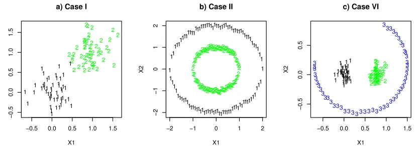
We considered five simulation set-ups, covering a variety of scenarios, as described below.

Case I: two convex clusters in two dimensions (Figure 1a). We consider two somewhat overlap-ping clusters with the same spherical shape, which is ideal for the K-means. Specifically, we have n=100 observations, 50 from a bivariate Normal distributionN((0,0)′_{,0.33I)while the other 50}

fromN((1,1)′,0.33I).

Case II: two non-convex clusters in two dimensions (Figure 1b). In contrast to the previous case favoring the K-means, the second simulation set-up was the opposite. There were 2 clusters as two nested circles (distorted with some added noises), each with 100 observations (see the upper-left

panel in Figure 3). Specifically, for cluster 1, we hadxi1=−1+2(i−1)/99,xi2=si q

1−x2_i1+εi,

si=−1 or 1 with an equal probability,εirandomly drawn fromU(−0.1,0.1), fori=1, ...,100; for

cluster 2, similarly we hadxi1=−2+4(i−101)/99,xi2=si q

−0.5 0.0 0.5 1.0 1.5 −0.5 0.0 0.5 1.0 1.5 X1 X2 1 1 1 1 1 1 1 1 1 1 1 1 1 1 1 1 1 1 1 1 1 1 1 1 1 1 1 1 1 1 1 1 1 1 1 ₁1

1 1 1 1 1 1 1 1 1 1 1 1 1 2 2 2 2 2 2 2 2 2 2 2 2 2 2 2 2 2 2 2 2 2 2 2 2₂ 2

2 2 2 2 2 2 2 2 2 2 2 2 2 2 2 2 2 2 2 2 2 2 2 2 a) Case I

−2 −1 0 1 2

−2 −1 0 1 2 X1 X2 1 1 1 1 1 1 1 1 1 1 1 1 1 1 1 1 1 1 1 1 1 1 1 1 1 1 1 1 1 1 1 1 1 1 1 1 1 1 1 1 1 1 1 1 1 1 1 1 1 1 1 1 1 1 1 1 1 1 1 1 1 1 1 1 1 1 1 1 1 1 1 1 1 1 1 1 1 1 1 1 1 1 1 1 1 1 1 1 1 1 1 1 1 1 1 1 1 1 1 1 2 2 2 2 2 2 2 2 2 2 2 2 2 2 2 2 2 2 2 2 2 2 2 2 2 2 2 2 2 2 2 2 2 2 2 2 2 2 2 2 2 2 2 2 2 2 2 2 2 2 2 2 2 2 2 2 2 2 2 2 2 2 2 2 2 2 2 2 2 2 2 2 2 2 2 2 2 2 2 2 2 2 2 2 2 2 2 2 2 2 2 2 2 2 2 2 2 2 22 b) Case II

−0.5 0.0 0.5 1.0 1.5

−0.5 0.0 0.5 X1 X2 1 1 1 1 1 1 1 1 1 1 1 1 1 1 1 1 1 1 1 1 1 1 1 1 ₁ 1 1 1 11_{1 1}

1

1 1 11

111 1 1 1₁ 1 1 11 11 22 2₂ 2 2 2 2 2 2 2 2 2 2 2 2 2 2 2 2 2 2 2 222 2 2 22 2 2 2 2 2 2 2 2 2₂ 2₂2 2

22 2 2 2 2 3₃₃ 3₃ 3 33 33 3 3 3 3 3 3 3 3 3 3 3 3 3 3 3 3 3 3 3 3 3 3 3 3 3 3 3 3 3 3 3 3 3 3 3 3 3 3 3 3

c) Case VI

Figure 1: The first simulated data set in a) Case I, b) Case II and c) Case VI.

is similar to the “two-circle” case in Ng et al. (2002), but perhaps more challenging here with larger distances between some points within the same cluster.

Case III: a null case with only a single cluster in 10 dimensions. 200 observations were uni-formly distributed over a unit square independently in each of the 10 dimensions. This is scenario (a) in Tibshirani et al. (2001).

Case IV: four clusters in 3 dimensions. The four cluster centers were randomly drawn from N(0,5I) in each simulation; if any of their distance was less than 1.0, then the simulation was abandoned and re-run. In each cluster, 25 or 50 observations were randomly chosen, each drawn from a normal distribution with mean at the cluster center and the identity covariance matrix. This is scenario (c) in Tibshirani et al. (2001).

Case V: two elongated clusters in 3 dimensions. This is similar to scenario (e) in Tibshirani et al. (2001), but with a much shorter distance between the two clusters. Specifically, cluster one was generated as follows: 100 observations were generated be equally spaced along the main diagonal of a three dimensional cube, then independent normal variate with mean 0 and SD=0.1 were added to each coordinate of each of the 100 observations; that is,xi j=−0.5+ (i−1)/99+εi j,εi∼N(0,0.1)

for j=1, 2, 3 andi=1, ...,100. Cluster 2 was generated in the same way, but with a shift of 2, not 10, making it harder than that used in Tibshirani et al. (2001) in each dimension.

Case VI: three clusters in 2 dimension with two spherically shaped clusters inside 3/4 of a perturbed circle (Figure 1c). This is similar to a case in Ng et al. (2002). Specifically, for cluster 1, we generatedxi1=1.1 sin(2π[30+5(i−1)]/360)andxi2=0.8 sin(2π[30+5(i−1)]/360) +εi for

i=1, ...,50, whereεi was randomly drawn fromU(−0.025,0.025); 50 observations were drawn

from each of the two bivariate Normal distributions,N((0,0)′,0.1I)andN((0.8,0)′,0.1I).

Due to the conceptual similarity between our proposed PRclust and spectral clustering (Sclust), we also included the spectral clustering algorithm of Ng et al. (2002) as outlined below. First, calcu-late an affinity matrixA= (Ai j)with elementsAi j=exp(−||xi−xj||22/γ)for any two observations i6= j andAii=0, whereγis a scaling parameter to be determined. Second, calculate a diagonal

matrixD=Diag(D11, ...,Dnn)withDii=∑nj=1Ai j. Third, calculateL=D−1/2AD−1/2. Fourth, for

a specified number of clusters k, we stack the k top eigen-vectors (corresponding to thek largest eigen-values) ofLcolumn-wise to form ann×kmatrix, sayZk; normalize each row ofZk to have

a unitL2-norm. Finally, treating each row ofZk as an observation, we apply the K-means to form

k clusters. There are two tuning parametersγandk that have to be decided in the algorithm. We used the implementation in the R packagekernlab, which includes a method of Ng et al. (2002) to selectγautomatically; however, one has to specifyk. We applied the GCV(GDF) to selectkas for the K-means. Unfortunately the functionspecc()in the R packagekernlabwas not numerically stable and sometimes might break down (i.e., exiting with an error message), though it could work in a re-run with a different random seed; the error occurred more frequently with an increasingk. Hence we only considered its use in a few cases by restrictingkto 1 to 3.

To evaluate the performance of a clustering algorithm, we used the Rand index (Rand, 1971), adjusted Rand index (Hubert and Arabie, 1985) and Jaccard index (Jaccard, 1912), all measuring the agreement between estimated cluster memberships and the truth. Each index is between 0 and 1 with a higher value indicating a higher agreement.

3.2 Simulation Results

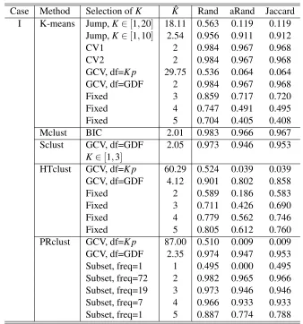
Case I: For the K-means, we chose the number of clusters using Jump, CV1, CV2 and GCV statis-tics; for comparison, we also fixed the number of clusters around its true value. The results are shown in Table 1. Both the Jump and GCV with the naive df=npmethods tended to select a too large number of clusters. In contrast, the GCV(GDF) performed extremely well: it always chose the correct K=2 clusters. Figure 2 shows how GDF and NDF changed with K, the number of clusters in the K-means algorithm, for the first simulated data set. Due to the adaptiveness of the K-means, GDF quickly increased to 150 withK<10 and approached the maximum df=np=200 forK=20. Since GDF was in general much larger than NDF, using GDF penalized more on more complex models (i.e., largerKin the K-means), explaining why GCV(GDF) performed much better than GCV(NDF).

Since the two clusters were formed by observations drawn from two Normal distributions, as expected, the model-based clustering Mclust performed best. In addition, the spectral clustering also worked well.

For PRclust, we searched τ∈ {0.1,0.2, ...,1} andλ2∈ {0.01,0.05,0.1,0.2,1}. PRclust with GCV(GDF) selecting its tuning parameters performed well too: the average number of clusters is close to the truthK0=2; the corresponding clustering results had high degrees of agreement with the truth, as evidenced by the high indices. Table 1 also displays the frequencies of the number of clusters selected by GCV(GDF): for the overwhelming majority (98%), either the correct number of clusterK0=2 was selected, or a slightly largerK=3 or 4 with veryhighagreement indices was chosen.

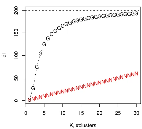
For the first (and a typical) simulated data set, we show how PRclust operated with various values of the tuning parameterλ2 (while λ1=1 and τ=0.5), yielding the solution path for ˆµi1,

Case Method Selection ofK Kˆ Rand aRand Jaccard I K-means Jump,K∈[1,20] 18.11 0.563 0.119 0.119

Jump,K∈[1,10] 2.54 0.956 0.911 0.912

CV1 2 0.984 0.967 0.968

CV2 2 0.984 0.967 0.968

GCV, df=K p 29.75 0.536 0.064 0.064 GCV, df=GDF 2 0.984 0.967 0.968

Fixed 3 0.859 0.717 0.720

Fixed 4 0.747 0.491 0.495

Fixed 5 0.704 0.405 0.408

Mclust BIC 2.01 0.983 0.966 0.967

Sclust GCV, df=GDF 2.05 0.973 0.946 0.953 K∈[1,3]

HTclust GCV, df=K p 60.29 0.524 0.039 0.039 GCV, df=GDF 4.12 0.901 0.802 0.858

Fixed 2 0.589 0.186 0.583

Fixed 3 0.711 0.426 0.690

Fixed 4 0.779 0.562 0.746

Fixed 5 0.805 0.612 0.760

PRclust GCV, df=K p 87.00 0.510 0.009 0.009 GCV, df=GDF 2.35 0.974 0.947 0.953 Subset, freq=1 1 0.495 0.000 0.495 Subset, freq=72 2 0.982 0.965 0.966 Subset, freq=19 3 0.973 0.946 0.946 Subset, freq=7 4 0.966 0.933 0.933 Subset, freq=1 5 0.887 0.774 0.788

Table 1: Simulation I results based on 100 simulated data sets with 2 clusters.

a sufficiently largeλ2, there were still quite some unequal ˆµi1’s, which were all remarkably near

their true values 0 or 1. In contrast, with the Lasso penalty, the estimated centroids were always shrunk towards each other, leading to their convergence to the same point at the end and thus much worse performance (Figure 3c). It is also noted that the solution paths with the Lasso penalty were almost linear, compared to the nearly step functions with the gTLP. Figure 3d) shows how HTclust worked. In particular, as pointed out by Ng et al. (2002), HTclust is not robust to outliers: since an “outlier” (lower left corner in Figure 1a) was farthest away from any other observations, it formed its own cluster while all others formed another cluster when the thresholdd was chosen to yield two clusters. This example demonstrates different operating characteristics between PRclust and HTclust, offering an explanation of the better performance of PRclust over HTclust.

0 5 10 15 20 25 30

0

50

100

150

200

K, #clusters

df

NNNNNN

NNNNNN

NNNNNN

NNNNNN

NNNNNN

G G

G G

G GG

GGG

GGGGG

GGGGGGGGGGGGGG

G

Figure 2: GDF (marked with ”G”) and NDF (marked with ”N”) versus the number of clusters,K, in the K-means algorithm for the first simulated data set in Case I. The horizontal line gives the maximum df=200.

to the cluster and its assigning a cluster membership of an observation based on its distance to the centroids; since the two clusters share the same centroid in truth, the K-means cannot distinguish the two clusters. Similarly, Mclust did not perform well.

As a comparison, perhaps due to the nature of the local shrinkage in estimating the centroids, PRclust worked much better than the above three methods, as shown in Table 2. Note that, the cluster memberships in PRclust are determined by the estimates ofθi j=µi−µj; due to the use of

the ridge penalty with a fixedλ1=1, we might have ˆθi j=0 but ˆµi6=µˆj.

Since HTclust assigned the cluster-memberships according to the pair-wise distances among the observations, not the nearest distance of an observation to the centroids as done in the K-means, it also performed well.

If the GCV(GDF) was used in Sclust, it would select ˆK=1 over ˆK=2, even though a specified ˆ

0.0 0.2 0.4 0.6 0.8 1.0

−0.5

0.0

0.5

1.0

1.5

λ₂

^ i1

a) PRclust−gTLP, λ_{1 1}

0.0 0.1 0.2 0.3 0.4 0.5 0.6

−0.5

0.0

0.5

1.0

1.5

λ₂

^ i1

b) PRclust2−gTLP, large λ₁

0.000 0.005 0.010 0.015

−0.5

0.0

0.5

1.0

1.5

λ₂

^ i1

c) PRclust−Lasso, λ

1 1

0.00 0.05 0.10 0.15 0.20 0.25 0.30 0.35

−0.5

0.0

0.5

1.0

1.5

d ^ i1

d) HTclust

Figure 3: Solution paths of ˆµi,1for a) PRclust (with gTLP), b) PRclust2, c) PRclust with the Lasso penalty and d) HTclust for the first simulated data set in Case I.

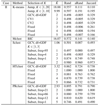
Case Method Selection ofK Kˆ Rand aRand Jaccard II K-means Jump,K∈[1,20] 18.88 0.557 0.111 0.110

Jump,K∈[1,10] 9.99 0.597 0.191 0.195 GCV, df=GDF 2 0.498 -0.005 0.329

CV1 2 0.498 -0.005 0.329

CV2 2 0.498 -0.005 0.329

Fixed 3 0.498 -0.006 0.261

Fixed 4 0.498 -0.008 0.194

Fixed 5 0.498 -0.007 0.166

Mclust BIC 16.07 0.572 0.141 0.140

Sclust GCV, df=GDF 1.06 0.501 0.007 0.493 K∈[1,3]

Subset, freq=95 1 0.497 0.000 0.497 Subset, freq=4 2 0.498 -0.005 0.329 Subset, freq=1 3 0.874 0.749 0.748

Fixed 2 0.980 0.960 0.973

HTclust GCV, df=GDF 3.32 0.862 0.724 0.738

Fixed 2 1.000 1.000 1.000

Fixed 3 0.881 0.763 0.762

Fixed 4 0.870 0.739 0.738

Fixed 5 0.866 0.732 0.731

PRclust GCV, df=GDF 2.93 0.895 0.791 0.790 Subset, freq=21 2 1.000 1.000 1.000 Subset, freq=66 3 0.880 0.759 0.759 Subset, freq=12 4 0.810 0.620 0.619 Subset, freq=1 5 0.746 0.491 0.490

Table 2: Simulation II results based on 100 simulated data sets with 2 clusters.

Cases III-IV: the simulation results are summarized in Table 3. All performed well for the null Case III. Case IV seems to be challenging with partially overlapping spherically shaped clusters of smaller cluster sizes: the number of clusters could be under- or over-selected by various methods. In terms of agreement, overall, as expected, the K-means with GCV(GDF) and Mclust performed best, closely followed by PRclust with GCV(GDF), which performed much better than HTclust.

Case Method Selection ofK Kˆ Rand aRand Jaccard III K-means GCV, df=GDF 1.00 1.000 1.000 1.000

Mclust BIC 1.00 1.000 1.000 1.000

Sclust GCV, df=GDF 1.00 1.000 1.000 1.000 K∈[1,3]

HTclust GCV, df=GDF 1.00 1.000 1.000 1.000 PRclust GCV, df=GDF 1.00 1.000 1.000 1.000 IV K-means GCV, df=GDF 3.48 0.880 0.748 0.728

CV1 3.10 0.789 0.575 0.581

CV2 4.22 0.790 0.558 0.561

Mclust BIC 3.50 0.883 0.753 0.732

HTclust GCV, df=GDF 6.49 0.589 0.352 0.452 PRclust GCV, df=GDF 4.75 0.790 0.612 0.628

Table 3: Simulation Cases III-IV results based on 100 simulated data sets with 1 and 4 clusters, respectively.

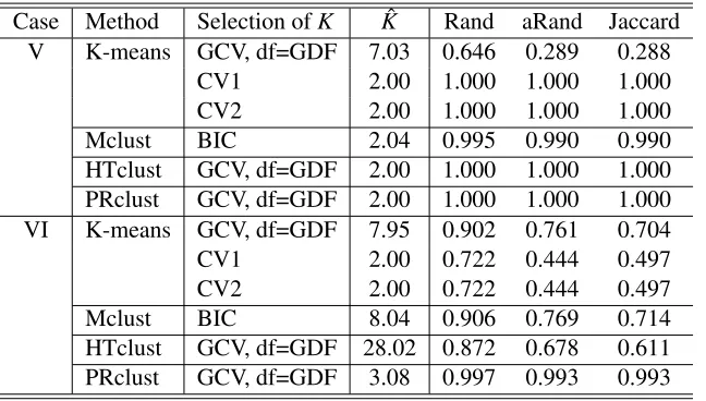
Case Method Selection ofK Kˆ Rand aRand Jaccard V K-means GCV, df=GDF 7.03 0.646 0.289 0.288

CV1 2.00 1.000 1.000 1.000

CV2 2.00 1.000 1.000 1.000

Mclust BIC 2.04 0.995 0.990 0.990

HTclust GCV, df=GDF 2.00 1.000 1.000 1.000 PRclust GCV, df=GDF 2.00 1.000 1.000 1.000 VI K-means GCV, df=GDF 7.95 0.902 0.761 0.704

CV1 2.00 0.722 0.444 0.497

CV2 2.00 0.722 0.444 0.497

Mclust BIC 8.04 0.906 0.769 0.714

HTclust GCV, df=GDF 28.02 0.872 0.678 0.611 PRclust GCV, df=GDF 3.08 0.997 0.993 0.993

Table 4: Simulation cases V-VI results based on 100 simulated data sets with 2 and 3 clusters, respectively.

divided an elongated cluster into several adjacent spherical clusters, which were then favored by GCV(GDF).

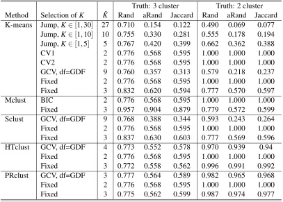
Truth: 3 cluster Truth: 2 cluster Method Selection ofK Kˆ Rand aRand Jaccard Rand aRand Jaccard K-means Jump,K∈[1,30] 27 0.710 0.154 0.122 0.490 0.069 0.077

Jump,K∈[1,10] 10 0.755 0.330 0.281 0.555 0.178 0.194 Jump,K∈[1,5] 5 0.767 0.420 0.399 0.662 0.362 0.388

CV1 2 0.776 0.568 0.595 1.000 1.000 1.000

CV2 2 0.776 0.568 0.595 1.000 1.000 1.000

GCV, df=GDF 9 0.760 0.357 0.313 0.579 0.218 0.237 Fixed 2 0.776 0.568 0.595 1.000 1.000 1.000 Fixed 3 0.832 0.620 0.594 0.777 0.570 0.597

Mclust BIC 2 0.776 0.568 0.595 1.000 1.000 1.000

Fixed 3 0.957 0.904 0.879 0.779 0.572 0.599 Sclust GCV, df=GDF 9 0.768 0.388 0.344 0.593 0.243 0.264 Fixed 2 0.776 0.568 0.595 1.000 1.000 1.000 Fixed 3 0.837 0.630 0.603 0.777 0.569 0.596 HTclust GCV, df=GDF 4 0.773 0.552 0.578 0.970 0.939 0.94

Fixed 2 0.776 0.568 0.595 1.000 1.000 1.000 Fixed 3 0.772 0.558 0.562 0.996 0.991 0.992 PRclust GCV, df=GDF 3 0.777 0.564 0.589 0.982 0.965 0.968 Fixed 2 0.776 0.568 0.595 1.000 1.000 1.000 Fixed 3 0.775 0.562 0.599 0.987 0.974 0.977

Table 5: Results for Fisher’s iris data with 2 or 3 clusters.

3.3 Iris Data

We applied the methods to the popular Fisher’s iris data. There are 4 measurements on the flower, sepal length, sepal width, petal length and petal width, for each observation. There are 50 obser-vations for each of the three iris subtypes. One subtype is well separated from the other two, but the latter two overlap with each other. For this data set, it is debatable whether there are 2 or 3 clusters; for this reason, for any clustering results, we calculated the agreement indices based on the 3 clusters (each corresponding to each iris subtype), and that based on only 2 clusters by combining the latter two overlapping subtypes into one cluster. Since two observations share an equal value on each variable, there are at most ˆK=149 clusters.

We standardized the data such that for each variable we had a sample mean 0 and SD=1. We applied the methods to the standardized data (p=4). We usedv=0.4; we tried a few other values ofvand obtained similar results for GDF. For the K-means, we tried the number of clustersK= 1,2, ...,30, each with 20 random starts. For HTclust, we searched 1000 candidated’s according to the empirical distribution of the pair-wise distances among the observations. For PRclust, we tried

λ2=∈ {0.1,0.2, ...,2}andτ2∈ {1.0,1.1, ...,2}. The results are shown in Table 5.

GCV(GDF) yielded ˆK=3 clusters with higher agreement indices than those of the K-means, Mclust and Sclust. HTclust selected ˆK=4 clusters with the agreement indices less than but close to those of PRclust. We also applied the K-means and Sclust with a fixed ˆK=2 or 3, and took the subset of the tuning parameter values yielding 2 or 3 clusters for HTclust and PRclust. It is interesting to note that, with ˆK=2, all the methods gave the same results that recovered the two true clusters; however, with ˆK=3, the results from PRclust and HTclust were similar, but different from the K-means and Sclust: the K-means and Sclust performed better in terms of the agreement with the 3 true clusters, but less well with the 2 true clusters, than PRclust and HTclust, demonstrating different operating characteristics between the K-means/Sclust and the other two methods. When fixed ˆK=3, Mclust gave the best results forK=3, suggesting the advantage of Mclust with overlapping and ellipsoidal clusters.

4. Further Modifications and Comparisons

We explore two well-motivated modifications to our new method, which turn out to be less competi-tive. Then we demonstrate the performance advantages of our new non-convex penalty over several existing convex penalties.

4.1 Modifications

In PRclust, so far we have fixedλ1=1, which cannot guarantee ˆθi j =µˆi−µˆj, even approximately

(Figure 3a). As an alternative, following Framework 17.1 of Nocedal and Wright (2000), we start the algorithm atλ1=1, at convergence we increase the value ofλ1, for example, by doubling its current value, and re-run the algorithm with the parameter estimates from the previous iteration as its starting values; this process is repeated until the convergence when the parameter estimates barely change. As before, we can use the new estimates ˆθi j’s to form clusters. We call this modified

method PRclust2. As shown in Figure 3b), for a sufficiently largeλ2, we’d have allθi j=0, leading

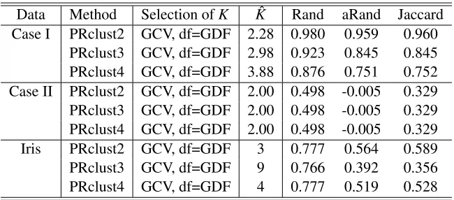
to all ˆµi1’s (almost) equal in PRclust2; in contrast, no matter how large λ2 was, we had multiple quite distinct ˆµi1’s in PRclust (Figure 3a). We applied PRclust2 to the earlier examples and obtained the following results: when all the clusters were convex, PRclust2 yielded results very similar to those of PRclust; otherwise, their results were different. Table 6 shows some representative results. It is surprising that PRclust performed better than PRclust2 for simulation Case II with two non-convex clusters. A possible explanation lies in their different estimates ofθi j’s, which are used by

both PRclust and PRclust2 to perform clustering. PRclust2 yields ˆθi j =µˆi−µˆj (approximately)

while PRclust does not. PRclust2 forms clusters based on the (approximate) equality of ˆµi’s, while

PRclust clusters two observationsi and j together if their ˆµi and ˆµj are close to each other, say,

||µˆi−µˆj||2<d0,i j, where the thresholdd0,i j is possibly(i,j)-specific. Hence, PRclust2 seems to be

more rigid and greedy in forming clusters than PRclust. Alternatively, we can regard PRclust as an early stopped and thus regularized version of PRclust2; it is well known that early stopping is an effective regularization strategy that avoids over-fitting in neural networks and trees (Hastie et al., 2001, p.326).

PRclust forms a cluster based on a connected component of a graph constructed with ˆθi j’s. More

generally, one can apply the spectral clustering of Ng et al. (2002) to either ˆµi’s or ˆθi j’s obtained

Data Method Selection ofK Kˆ Rand aRand Jaccard Case I PRclust2 GCV, df=GDF 2.28 0.980 0.959 0.960

PRclust3 GCV, df=GDF 2.98 0.923 0.845 0.845 PRclust4 GCV, df=GDF 3.88 0.876 0.751 0.752 Case II PRclust2 GCV, df=GDF 2.00 0.498 -0.005 0.329 PRclust3 GCV, df=GDF 2.00 0.498 -0.005 0.329 PRclust4 GCV, df=GDF 2.00 0.498 -0.005 0.329 Iris PRclust2 GCV, df=GDF 3 0.777 0.564 0.589 PRclust3 GCV, df=GDF 9 0.766 0.392 0.356 PRclust4 GCV, df=GDF 4 0.777 0.519 0.528

Table 6: Results for modified PRclust for 100 simulated data sets (2 clusters) or the iris data (3 clusters).

data examples; as shown in Table 6, the two methods did not improve over the original PRclust. As a reviewer suggested, alternatively, we may also apply PRclust, not the K-means, to the eigen-vectors in a modified Sclust; however, it will be challenging to develop computationally more efficient methods to simultaneously choose multiple tuning parameters, that is,(γ,k)in Sclust and(λ2,τ)in PRclust.

4.2 Comparison with Some Convex Fusion Penalties

In contrast to our non-convex gTLP penalty, several authors have studied the use of theLq

-norm-based convex fusion penalties. Pelckmans et al. (2005) proposed using a fusion penalty -norm-based on theLq-norm with the objective function

1 2

n

∑

||xi−µi||22+λ

∑

i<j

||µi−µj||q,

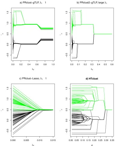
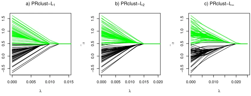
and proposed an efficient quadratic convex programming-based computing method forq=1. Lind-sten et al. (2011) recognized the importance of using a group penalty withq>1, and applied the Matlab CVX package (Grant and Boyd, 2011) to solve the general convex programming problem for the group Lasso penalty withq=2 (Yuan and Lin, 2006). Hocking et al. (2011) exploited the piecewise linearity of the solution paths forq=1 orq=∞, and proposed an efficient algorithm for each ofq=1, 2 and∞respectively. We call these methods PRclust-Lq. Note that PRclust-L1 corre-sponds to our PRclust-Lasso, for which (and our default PRclust-gTLP) however we have proposed a different computing algorithm, the quadratic penalty method. Importantly, due to the use of the convex penalty, the solution path of PRclust-Lqis quite different from that of PRclust-gTLP. Using

the Matlab CVX package, we applied PRclust-Lqwithq∈ {1,2,∞}to simulation Case I; the results

for the first data set are shown in Figure 4. It is clear that the solution path of PRclust-L1(Figure 4a) was essentially the same as that of PRclust-Lasso (Figure 3c) (while different computing algorithms were applied). More importantly, overall the solution paths of all three PRclust-Lq were similar to

0.000 0.005 0.010 0.015

−0.5

0.0

0.5

1.0

1.5

λ

^ i1

a) PRclust−L1

0.000 0.005 0.010 0.015 0.020

−0.5

0.0

0.5

1.0

1.5

λ

^ i1

b) PRclust−L2

0.000 0.010 0.020

−0.5

0.0

0.5

1.0

1.5

λ

^i1

c) PRclust−L∞

Figure 4: Solution paths of ˆµi,1 for PRclust-Lq with a)q=1, b)q=2 and c) q=∞for the first

simulated data set in Case I.

difficult to correctly select the number of clusters. In fact, both Pelckmans et al. (2005) and Hocking et al. (2011) treated PRclust-Lq as a hierarchical clustering tool; none of the authors discussed the

choice of the number of clusters. The issue of anLq-norm penalty in yielding possibly severely

bi-ased estimates is well known in penalized regression, which partially motivated the development of non-convex penalties such as TLP (Shen et al., 2012). In the current context, Lindsten et al. (2011) has recognized the issue of the biased centroid estimates in PRclust-Lqand thus proposed a second

stage to re-estimate the centroids after a clustering result is obtained. In contrast, with the use of the non-convex gTLP, the above issues are largely avoided as shown in Figure 3ab).

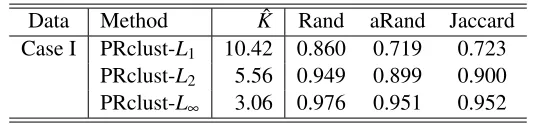
When we applied the GCV(GDF) to select the number of clusters for PRclust-Lqin simulation

Case I, as expected, it performed poorly. Hence, for illustration, we considered an ideal (but not practical) alternative. For any d0≥0, similar to hierarchical clustering, we defined an adjacency matrixA= (ai j)withai j=I(||µˆi−µˆj||2≤d0); any two observationsxiandxjwere assigned to the

same cluster ifai j=1. Then for any givenλ>0 andd0∈ {10−1,10−2,10−3,10−4,0}, we calculated the Rand index for the corresponding PRclust-Lqresults and thetruecluster memberships. We show

the results of PRclust-Lqwith the values of (λ,d0)achieving the maximum Rand index, giving an

upper bound on the performance of PRclust-Lqwith any practical criterion to select the number of

clusters. As shown in Table 7, a larger value ofqseemed to give better ideal performance of PRclust-Lq; when compared to PRclust-gTLP (Table 1), none of the three PRclust-Lq methods, even in the

ideal case of using the true cluster memberships to select the number of clusters, performed better in selecting the correct number of clusters than PRclust-gTLP with the GCV(GDF) criterion.

5. Discussion

un-Data Method Kˆ Rand aRand Jaccard Case I PRclust-L1 10.42 0.860 0.719 0.723

PRclust-L2 5.56 0.949 0.899 0.900 PRclust-L∞ 3.06 0.976 0.951 0.952

Table 7: Results for PRclust-Lq with ˆK selected by maximizing the Rand index for 100 simulated

data sets (2 clusters) in Case I.

suitable or difficult to the K-means, such as in the presence of non-convex clusters, as demonstrated in our simulation Case II (Table 2). Similarly, Mclust does not perform well for non-convex clusters (Table 2), but may have advantages with overlapping and ellipsoidal clusters as for simulation Case I (Table 1) and the iris data (Table 5). There is also some similarity between PRclust and HTclust (or single-linkage hierarchical clustering). Although much simpler, HTclust does not have any mecha-nism for shrinkage estimation, and in general did not perform better than PRclust in our examples. Between PRclust and spectral clustering, it seems that they are complementary to each other, though it remains challenging to develop competitive model selection criteria for spectral clustering. For example, our results demonstrated the effectiveness of the method of Ng et al. (2002) in selecting the scale parameterγ, but the clustering result also critically depended on the specifiedk, the number of clusters, for which the GCV(GDF) might not perform well. Although Zelnik-Manor and Perona (2004) have proposed a model selection criterion to self-tune the two parametersγandk>1, it does not work fork=1; ifk=1 is included, the criterion will always selectk=1. More generally, model selection is related to kernel learning in spectral clustering (Bach and Jordan, 2006). It is currently an open problem whether the strengths of PRclust and spectral clustering can be combined.

PRclust can be extended in several directions. First, rather than the squared error loss, we can use other loss functions. Corresponding to modifying the K-means to the K-medians, K-midranges or K-modes (Steinley, 2006), we can use anL1,L∞ andL0 loss function, respectively. Computa-tionally, an efficient coordinate-wise algorithm can be implemented for penalized regression with anL1loss (Friedman et al., 2007; Wu and Lange, 2008), but it is unclear how to do so for the other two. K-median clustering is closely related to partitioning-around-centroids (PAM) of Kaufman and Rousseeuw (1990), and is more robust to outliers than is the K-means. A modification of PRclust along this direction may retain this advantage. Second, rather than assuming spherically shaped clusters, as implicitly used by the K-means, we can use a general covariance matrixV with a loss function

L(xi−µi) =

1

2(xi−µi)

′_V−1_(x

i−µi),

where V is either given or to be estimated. A non-identityV allows a more general model of ellipsoidal clusters. Alternatively, we can also relax the equal cluster volume assumption and use:

L(xi−µi) =

1

2(xi−µi)

′_(x

i−µi)/σ2i,

where observation-specific variances σ2

i’s have to be estimated through grouping pursuit, as for

observation-specific means/centroidsµi’s (Xie et al., 2008). More generally, corresponding to the

and Peel, 2002), we might use

L(xi−µi) =

1

2(xi−µi)

′_V−1

i (xi−µi),

for a general and observation-specific covariance matrixVi, though it will be challenging to adopt a

suitable grouping strategy to estimateVi’s effectively. Among others, it might provide a

computa-tionally more efficient algorithm than the EM algorithm commonly adopted in mixture model-based clustering (Dempster et al., 1977). Equally, we may accordingly modify the RSS term in GCV so that it will not overly favor spherically shaped clusters. Third, in our current implementation, after parameter estimation, we construct an adjacency matrix and search connected components in the corresponding graph to form clusters. This is a special and simple approach to more general graph-based clustering (Xu and Wunsch, 2005); other more sophisticated approaches may be borrowed or adapted. We implemented a specific combination of PRclust and spectral clustering along with GCV(GDF) for model selection: we first applied PRclust, then used its output as the input to spec-tral clustering, but it did not show improvement over PRclust. Other options exist; for example, as suggested by a reviewer, it might be more fruitful to replace the K-means in spectral clustering with PRclust. These problems need to be further investigated. Fourth, in the quadratic penalty method, rather than fixingλ1=1 or allowingλ1→∞, we may want to treatλ1as a tuning parameter; a chal-lenge is to develop computationally more efficient methods (e.g., than data perturbation-based GCV estimation) to select multiple tuning parameters. Alternatively, as a reviewer suggested, we may also apply the alternating direction method of multipliers (ADMM) (Boyd et al., 2011), which is closely related to, but perhaps more general and simpler than the quadratic penalty method. Finally, we have not applied the proposed method to high-dimensional data, for which variable selection is nec-essary. In principle, we may add a penalty into our objective function for variable selection (Pan and Shen, 2007), which again requires a fast method to select more tuning parameters and is worth future investigation.

Perhaps the most interesting idea of our proposal is the view of regarding clustering analysis as a penalized regression problem, blurring the typical line drawn to distinguish clustering (or unsu-pervised learning) with regression and classification (i.e., suunsu-pervised learning). This not only opens a door to using various regularization techniques recently developed in the context of penalized regression, such as novel non-convex penalties and algorithms, but also facilitates the use of other model selection techniques. In particular, we find that our proposed regression-based GCV with GDF is promising for the K-means and PRclust (but perhaps not for spectral clustering) in selecting the number of clusters, a hard and interesting problem in itself; since this is not the main point of this paper, we wish to report more on this topic elsewhere.

Acknowledgments

Appendix A.

We prove Theorem 1 in Section 2.2.

By construction ofS(m)(µ,θ)and the definition of minimization, for eachm∈N,

0 ≤ S(ˆµ(m),θˆ(m)) =S(m+1)(µˆ(m),θˆ(m))≤S(m)(µˆ(m),θˆ(m))

≤ S(m)(µˆ(m),θˆ(m−1))≤S(m)(ˆµ(m−1),θˆ(m−1)) =S(µˆ(m−1),θˆ(m−1)),

implying that S(ˆµ(m),θˆ(m)_{) decreases in m. Note that S(µˆ}(m)_,θˆ(m)_{)≥0 for all m. Then it} con-verges, andS(µˆ(m)_,θˆ(m)_{)must decreases strictly inmbefore meeting the stopping rule to terminate.} Moreover, by construction,S(m+1)(µ,θ)has only a finite number of distinctly different functions in m. This implies thatS(m+1)(µˆ(m),θˆ(m)_{) =S(ˆµ}(m)_,θˆ(m)_{) has a finite number of different minimizers} across allm∈N, hence termination must occur finitely.

To show that(µˆ(m⋆),θˆ(m⋆)_{) is a local minimizer ofS(µ,θ), we check if it satisfies a local} opti-mality ofS(µ,θ), defined by regular subdifferentials (Rockafellar and Wets, 2003):

[1+λ1(n−1)]µi−xi−λ1

∑

j>i

(µj+θi j)−λ1

∑

j<i

(µj−θji) =0,i=1, ...,n, (4)

−λ1(µi−µj−θi j) +λ2bi j θi j

||θi j||2

=0, i,j=1, ...,n(i< j), (5)

where bi j is the regular subdifferential of min(||θi j||2,τ) at ||θi j||2. Note that (µˆ(m

⋆₎

,θˆ(m⋆)_{) =} (µˆ(m⋆−1),θˆ(m⋆−1)_{)at termination. Then (4) is satisfied with(µ,θ) = (µˆ}(m⋆−1)_,θˆ(m⋆−1)_{). For (5), we} discuss three cases. If||_θˆ(m⋆−1)

i j ||2>τ, then ˆθ(m

⋆₋₁₎

i j =µˆ

(m⋆)

i −µˆ

(m⋆)

j , implying (5) whenθi j=θˆ(m

⋆₎

i j

becausebi j=0. If 0<||θˆ(m

⋆₎

i j ||2<τand||µˆ(m

⋆₎

i −µˆ

(m⋆)

j ||2≥λ_λ2₁, then ˆ

θ_{i j}(m⋆)= (||µˆ_i(m⋆)−µˆ(_jm⋆)||2−

λ2

λ1 ) µˆ

(m⋆)

i −µˆ

(m⋆)

j

||µˆ(_im⋆)−µˆ(_jm⋆)||2 ,

hence that||θˆ_{i j}(m⋆)||2=||µˆ(m

⋆₎

i −µˆ

(m⋆)

j ||2−

λ2

λ1. Then (4) is met whenθi j =

ˆ

θ(_{i j}m⋆)becausebi j=1. If

0<||θˆ(_{i j}m⋆)||2<τand||µˆ(m

⋆₎

i −µˆ

(m⋆)

j ||2<λ_λ2₁, then||θˆ(m

⋆₎

i j ||2=0, which is contrary to the fact that 0<||_θˆ(m⋆)

i j ||2<τ. This completes the proof. Appendix B.

We prove the equivalence between HTclust and the single-linkage hierarchical clustering (SL-Hclust).

References

L. An and P. Tao. Solving a class of linearly constrained indefinite quadratic problems by D.C. algorithms.J. Global Optimization, 11:253-285, 1997.

F.R. Bach and M.I. Jordan. Learning spectral clustering, with application to speech separation. Journal of Machine Learning Research, 7:1963-2001, 2006.

J.D. Banfield and A.E. Raftery. Model-based Gaussian and non-Gaussian clustering. Biometrics, 49:803-821, 1993.

S. Boyd, N. Parikh, E. Chu, B. Peleato and J. Eckstein. Distributed optimization and statistical learning via the alternating direction method of multipliers.Foundations and Trends in Machine Learning, 3(1):1-122, 2011.

A.P. Dempster, N.M. Laird and D.B. Rubin. Maximum likelihood from incomplete data via the EM algorithm (with discussion).JRSS-B, 39:1-38, 1977.

J. Fan and R. Li. Variable selection via nonconcave penalized likelihood and it oracle properties. JASA, 96:1348-1360, 2001.

C. Fraley and A.E. Raftery. MCLUST Version 3 for R: Normal Mixture Modeling and Model-Based Clustering. Technical Report no. 504, Department of Statistics, University of Washington. 2006.

J. Friedman, T. Hastie, H. Hofling and R. Tibshirani. Pathwise coordinate optimization.Ann Appl Statistics, 2:302-332, 2007.

G.H. Golub, M. Heath and G. Wahba. Generalized cross-validation as a method for choosing a good ridge parameter.Technometrics, 21:215-223, 1979.

M. Grant and S. Boyd. CVX: Matlab software for disciplined convex programming, version 1.21, 2011.http://cvxr.com/cvx

T. Hastie, R. Tibshirani and J. Friedman.The Elements of Statistical Learning: Data Mining, Infer-ence, and Prediction. Springer-Verlag, 2001.

T. Hocking, A. Joulin, F. Bach and J.-P. Vert. Clusterpath: An Algorithm for Clustering using Con-vex Fusion Penalties. In L. Getoor and T. Scheffer (Eds.),Proceedings of the 28th International Conference on Machine Learning (ICML’11), p.745-752, 2011.

L. Hubert and P. Arabie. Comparing partitions.Journal of Classification, 2:193-218, 1985.

P. Jaccard. The distribution of flora in the alpine zone.New Phytologist., 11:37-50, 1912.

L. Kaufman and P.J. Rousseeuw. Finding Groups in Data: An Introduction to Cluster Analysis. Wiley, New York, 1990.

G.J. McLachlan and D. Peel.Finite Mixture Model.New York, John Wiley & Sons, Inc. 2002.

A. Ng, M. Jordan and Y. Weiss. On spectral clustering: analysis and an algorithm.NIPS, 2002.

J. Nocedal and S.J. Wright.Numerical Optimization. Springer, 2000.

W. Pan and X. Shen. Penalized model-based clustering with application to variable selection. Jour-nal of Machine Learning Research, 8:1145-1164, 2007.

K. Pelckmans, J. De Brabanter, J.A.K. Suykens and B. De Moor. Convex Clustering Shrinkage. Workshop on Statistics and Optimization of Clustering Workshop (PASCAL), London, U.K., Jul. 2005. Available at ftp://ftp.esat.kuleuven.ac.be/pub/SISTA/kpelckma/ccs pelckmans2005.pdf.

W.M. Rand. Objective criteria for the evaluation of clustering methods.JASA, 66:846-850, 1971.

R.T. Rockafellar and R.J. Wets.Variational Analysis. Springer-Verlag, 2003.

X. Shen and J. Ye. Adaptive model selection.JASA, 97:210-221, 2002.

X. Shen and H.-C. Huang. Grouping pursuit through a regularization solution surface. JASA, 105:727-739, 2010.

X. Shen, W. Pan and Y. Zhu. Likelihood-based selection and sharp parameter estimation. JASA, 107:223-232, 2012.

D. Steinley. K-means clustering: a half-century synthesis. British Journal of Mathematical and Statistical Psychology, 59:1-34, 2006.

C.A. Sugar and G.M. James. Finding the number of clusters in a data set: An information theoretic approach.Journal of the American Statistical Association, 98:750-763, 2003.

A. Thalamuthu, I. Mukhopadhyay, X. Zheng and G.C. Tseng. Evaluation and comparison of gene clustering methods in microarray analysis.Bioinformatics, 22:2405-2412, 2006.

R. Tibshirani. Regression shrinkage and selection via the lasso.JRSS-B, 58:267-288, 1996.

R. Tibshirani, M. Saunders, S. Rosset, J. Zhu and K. Knight. Sparsity and smoothness via the fused lasso.JRSS-B, 67:91-108, 2005.

R. Tibshirani, G. Walther and T. Hastie. Estimating the number of clusters in a data set via the gap statistic.JRSS-B, 63:411-423, 2001.

P. Tseng. Convergence of block coordinate descent method for nondifferentiable maximization.J. Opt. Theory Appl., 109:474-494, 2001.

J. Wang. Consistent selection of the number of clusters via crossvalidation.Biometrika, 97:893-904, 2010.

B. Xie, W. Pan and X. Shen. Penalized model-based clustering with cluster-specific diagonal co-variance matrices and grouped variables.Electronic Journal of Statistics, 2:168-212, 2008.

R. Xu and D. Wunsch. Survey of clustering algorithms.IEEE Trans Neural Networks, 16:645-678, 2005.

J. Ye. On measuring and correcting the effects of data mining and model selection.JASA, 93:120-131, 1998.

M. Yuan and Y. Lin. Model selection and estimation in regression with grouped variables.JRSS-B, 68:49-67, 2006.