Optimal Discovery with Probabilistic Expert Advice: Finite Time Analysis and Macroscopic Optimality

Optimal Discovery with Probabilistic Expert Advice:

Finite Time Analysis and Macroscopic Optimality

S´ebastien Bubeck [email protected]

Department of Operations Research and Financial Engineering Princeton University

Princeton, NJ, 08544, USA

Damien Ernst [email protected]

Department of Electrical Engineering and Computer Science University of Li`ege, Institut Montefiore, B28

B-4000 Li`ege, Belgium

Aur´elien Garivier [email protected] Institut de Math´ematiques de Toulouse

Universit´e Paul Sabatier 118, route de Narbonne

F-31062 Toulouse Cedex 9, France

Editor:Nicolo Cesa-Bianchi

Abstract

We consider an original problem that arises from the issue of security analysis of a power system and that we name optimal discovery with probabilistic expert advice. We address it with an algo-rithm based on the optimistic paradigm and on the Good-Turing missing mass estimator. We prove two different regret bounds on the performance of this algorithm under weak assumptions on the probabilistic experts. Under more restrictive hypotheses, we also prove a macroscopic optimality result, comparing the algorithm both with an oracle strategy and with uniform sampling. Finally, we provide numerical experiments illustrating these theoretical findings.

Keywords: optimal discovery, probabilistic experts, optimistic algorithm, Good-Turing estimator, UCB

1. Introduction

In this paper we consider the following problem: Let

X

be a set, andA_⊂

X

be a set of interesting elements in

X

. One can access

X

only through requests to a finite set of probabilistic experts. More precisely, when one makes a request to theith expert, the latter draws independently at random a point from a fixed probability distribution Pi over

X

. One is interested in discovering rapidly as

many elements ofAas possible, by making sequential requests to the experts.

1.1 Motivation

hours). Once those dangerous contingencies have been identified, the system operators usually take preventive actions so as to ensure that they could mitigate their effect on the system in the likelihood they would occur. Note that usually, the dangerous contingencies are very rare with respect to the non dangerous ones. A straightforward approach for tackling this security analysis problem is to simulate the power system dynamics for every credible contingency so as to identify those that are indeed dangerous. Unfortunately, when the set of credible contingencies contains a large number of elements (say, there are more than 105_{credible contingencies) such an approach may not possible} anymore since the computational resources required to simulate every contingency may excess those that are usually available during the few (tens of) minutes available for the real-time security anal-ysis. One is therefore left with the problem of identifying within this short time-frame a maximum number of dangerous contingencies rather than all of them. The approach proposed in Fonteneau-Belmudes (2012) and Fonteneau-Fonteneau-Belmudes et al. (2010) addresses this problem by building first very rapidly what could be described as a probability distributionPover the set of credible contin-gencies that points with significant probability to contincontin-gencies which are dangerous. Afterwards, this probability distribution is used to draw the contingencies to be analyzed through simulations. When the computational resources are exhausted, the approach outputs the contingencies found to be dangerous. One of the main shortcoming of this approach is that usuallyPpoints only with a significant probability to a few of the dangerous contingencies and not all of them. This in turn makes this probability distribution not more likely to generate after a few draws new dangerous contingencies than for example a uniform one. The dangerous contingencies to which P points to with a significant probability depend however strongly on the set of (sometimes arbitrary) en-gineering choices that have been made for building it. One possible strategy to ensure that more dangerous contingencies can be identified within a limited budget of draws would therefore be to considerK>1 sets of engineering choices to buildKdifferent probability distributionsP1,P2,. . ., PK and to draw the contingencies from these K distributions rather than only from a single one.

This strategy raises however an important question to which this paper tries to answer: how should the distributions be selected for being able to generate with a given number of draws a maximum number of dangerous contingencies? We consider the specific case where the contingencies are se-quentially drawn and where the distribution selected for generating a contingency at one instant can be based on the past distributions that have been selected, the contingencies that have been already drawn and the results of the security analyses (dangerous/non dangerous) for these contingencies. This corresponds exactly to the optimal discovery problem with expert advice described above. We believe that this framework has many other possible applications, such as for example web-based content access.

1.2 Setting and Notation

In this paper we restrict our attention to finite or countably infinite sets

X

. We denote by K the number of experts. For eachi_{∈ {}1, . . . ,K_}, we assume that(Xi,n)n≥1 are random variables with distributionPisuch that the(Xi,n)i,nare independent. Sequential discovery with probabilistic expert

advice can be described as follows: at each time stept_∈N∗_{, one picks an indexIt∈ {1, . . . ,K}, and}

one observesXIt,n_It,t, where

ni,t =

∑

s≤t

The goal is to choose the(It)t≥1so as to observe as many elements ofAas possible in a fixed horizon t, that is to maximize the number of interesting items found aftertrequests

F(t) =

∑

x∈A

1

x_{∈ {}X1,1, . . . ,X1,n1,t, . . . ,XK,1, . . . ,XK,nK,t}

. (1)

Note in particular that it is of no interest to observe twice the same same element ofA. The in-dex It+1 may be chosen according to past observations: it is a (possibly randomized) function of

(I1,XI1,1, . . . ,It,XIt,nIt,t).

An easier quantity to analyze than the number of interesting items found F(t) is the waiting timeT(λ),λ_∈(0,1), which is the time at which the strategy has a missing mass of interesting items smaller thanλon every experts, that is

T(λ) =inf

t:_∀i_{∈ {}1, . . . ,K_},Pi(A\ {X1,1, . . . ,X1,n1,t, . . . ,XK,1, . . . ,XK,nK,t})≤λ

. (2)

While we shall derive a general strategy that can be used without any assumption on the prob-abilistic experts, for the mathematical analysis of the waiting time T(λ) we make the following assumption:

(i) non-intersecting supports:A_∩supp(Pi)∩supp(Pj) =/0fori6= j.

Furthermore we will also derive some results under the following more restrictive assumptions:

(ii) finite supports with the same cardinality:_|supp(Pi)|=N,∀i∈ {1, . . . ,K},

(iii) uniform distributions:Pi(x) =_N1,∀x∈supp(Pi),∀i∈ {1, . . . ,K}.

1.3 Contribution and Content of the Paper

This paper contains the description of a generic algorithm for the optimal discovery problem with probabilistic expert advice, and a theoretical analysis of its properties. In Section 2, we first depict our strategy, termed Good-UCB. This algorithm relies on the optimistic paradigm, which led to the UCB (Upper Confidence Bound) algorithm for multi-armed bandits, see Auer et al. (2002) and Garivier and Capp´e (2011). It relies also on a finite-time analysis of the Good-Turing estimator for the missing mass. We also derive in Section 2 two different regret bounds under the non-intersecting assumption (i): we first show thatFUCB(t)(the number of interesting items found by Good-UCB) is larger thanF∗(t)(the number of interesting items found by an oracle strategy), up to a term of order

p

Ktlog(t). We argue that such a bound does not capture all the fine properties of Good-UCB: indeed, on the contrary to the multi-armed bandit problem, here the regret F∗(t)₋F(t) remains bounded for any reasonable strategy. This can be understood as arestoring propertyof the game: if a policy makes a sub-optimal choice at some given timet, then in the future it will have better opportunities than the optimal policy. This key feature of our problem prevents the regret from growing too much. To analyze this phenomenon, we complete our first bound by a second regret analysis—the main result of the paper—which states roughly that with high probability, TUCB(λ)

(the waiting time for the strategy Good-UCB) isuniformly(inλ) smaller thanT∗(λ′)(the smallest possible waiting time), for someλ′_{close toλand up to a small additional term, see Theorem 5 for}

In Section 3 we propose to investigate the behavior of Good-UCB in amacroscopic limitsense, that is we make assumptions [(i), (ii), (iii)] and we consider the limit when the size of the set

X

grows to infinity while maintaining a constant proportion of interesting items. In this scenario we show that Good-UCB is macroscopically optimal, in the sense that the normalized waiting time of Good-UCB tends to the normalized smallest possible waiting time. We also derive a formula for this latter quantity and we show that it is equal to∑i:qi>λlogqiλ, whereqiis the limiting proportion of

interesting items on experti. This macroscopic limit also allows to easily assess the performance of different strategies, and we show that for example the normalized waiting time of uniform sampling tends toKmax1≤i≤Klogqi_λ, which proves that this strategy is macroscopically suboptimal, unless all

experts have the same number of interesting items.

Finally, Section 4 reports experimental results that show that the Good-UCB algorithm performs very well, even in a setting where assumptions (i), (ii) and (iii) are not satisfied. The appendix contains some technical proofs, together with a more detailed discussion on oracle strategies in the macroscopic limit and on the relation between the waiting time T defined in (2) and the number of items found F defined in (1), proving in particular that optimality in terms of waiting time is equivalent to optimality in terms of number of items found.

2. The Good-UCB Algorithm

We describe here the Good-UCB strategy. This algorithm is a sequential method estimating at timet, for each experti_{∈ {}1, . . . ,K_}, the total probability of the interesting items that remain to be discovered through requests to expert i. This estimation is done by adapting the so-called Good-Turing estimator for the missing mass. Then, instead of simply using the distribution with highest estimated missing mass, which proves hazardous, we make use of the optimistic paradigm—see Bubeck and Cesa-Bianchi (2012, Chapter 2, and references therein)—a heuristic principle well-known in reinforcement learning, which entails to prefer using anupper-confidence bound(UCB) of the missing mass instead. At a given time step, the Good-UCB algorithm simply makes a request to the expert with highest upper-confidence bound on the missing mass at this time step.

We start in Section 2.1 with the Good-Turing estimator and a brief study of its concentration properties. Then we describe precisely the Good-UCB strategy in Section 2.2. Next we proceed to the theoretical analysis of Good-UCB and we start in Section 2.3 where we describe an oracle strategy (that we shall use as a comparator) that we prove to be optimal under assumption (i). In Section 2.4 we show that one can obtain a standard regret bound of order√twhen one compares the number of itemsFUCB_{(t)found by Good-UCB to the number of itemsF}∗_{(t) found by the oracle.}

This bound is not completely satisfactory (as we explain in Section 2.4), and our main result—a ’non-linear’ regret bound—is proved in Section 2.5.

2.1 Estimating the Missing Mass

ofΩdrawn independently under the same distributionP, and define for everyx∈Ω:

On(x) = n

∑

m=1

1{Xm=x}, Zn(x) =1{On(x) =0}, Un(x) =1{On(x) =1}.

LetRn=∑x_∈AZn(x)P(x)denote the missing mass of the interesting items, and letUn=∑x_∈AUn(x)

be the number of elements of A that have been seen exactly once (in linguistics, they are often called hapaxes). The idea of the Good-Turing estimator—see Good (1953), see also McAllester and Schapire (2000); Orlitsky et al., and references therein—is to estimate the (random) “missing mass”Rn, which is the total probability of all the interesting items that do not occur in the sample

X1, . . . ,Xn, by the “fraction of hapaxes ˆRn=Un/n. This estimator is well-known in linguistics, for

instance in order to estimate the number of words in some language, see Gale and Sampson (1995). We shall use the following tight bound on the estimation error. We emphasize the fact that the following bound holds trueindependently of the underlying distribution P.

Proposition 1 With probability at least1₋δ,

ˆ Rn−

1 n−(1+

√ 2)

r

log(4/δ)

n ≤Rn≤Rˆn+ (1+ √

2)

r

log(4/δ)

n .

Proof For self-containment, we first show thatE_Rn−E_Rˆ_n∈−1 n,0

; this result is well known, see for example Theorem 1 in McAllester and Schapire (2000):

E_Rn−E_Rˆ_n=

∑

x∈A

P(x) (1₋P(x))n₋1

n×nP(x) (1−P(x))

n−1

=₋1

n_x

∑

_∈AP(x)×nP(x) (1−P(x))

n−1

=₋1

nE

"

∑

x∈A

P(x)Un(x)

#

∈

−1 n,0

.

Next we apply the inequality of McDiarmid (1989) to ˆRn as follows. The random variable ˆRn

is a function of the independent observations X1, . . . ,Xn such that, denoting ˆRn = f(X1, . . . ,Xn),

modifying just one observation has limited impact:_∀l_{∈ {}1, . . . ,n_},_∀(x1, . . . ,xn,x′_l)∈Ωn+1,

f(x₁, . . . ,x_n)−f(x₁, . . . ,x_l−1,x′_l,x_l+1, . . . ,x_n) ≤

2 n.

Thus one gets that, with probability at least 1₋δ,

Rˆ_n−E[Rˆ_n] ≤

r

2 log(2/δ)

n .

Finally we extract the following result from Theorem 10 and Theorem 16 in McAllester and Ortiz (2003): with probability at least 1₋δ,

|Rn−E[Rn]| ≤

r

log(2/δ)

n .

2.2 The Good-UCB Algorithm

Following the example of the well-known Upper-Confidence Bound procedure for multi-armed bandit problems, we propose Algorithm 1, which we callGood-UCBin reference to the estimator it relies on. For each armi_{∈ {}1, . . . ,K_}, the index at timetof Good-UCB corresponds to the estimate

ˆ

Ri,ni,t−1=

1 ni,t−1_x

∑

_∈A

1

(_ni

,t−1

∑

s=1

1{Xi,s=x}=1 and

K

∑

j=1

nj,t−1

∑

s=1

1{Xj,s=x}=1

)

of the missing mass

∑

x∈A\nXI₁,_nI

1,1,...,XIt−1,nIt−1,t−1 o

Pi(x) (3)

inflated by a confidence bonus of orderplog(t)/ni,t−1. Good-UCB relies on a tuning parameterC which is discussed below.

Algorithm 1Good-UCB 1: For 1_≤t_≤KchooseIt =t.

2: fort_≥K+1do

3: ChooseIt =arg max1≤i≤K

n

ˆ

Ri,ni,t−1+C

q

log(4t)

ni,t−1

o

4: ObserveXt distributed asPIt and update the missing mass estimates accordingly

5: end for

The Good-UCB algorithm is designed to work without any assumption on the probabilistic ex-perts. However for the analysis we shall make the non-intersecting supports assumption (i). Indeed without this assumption the missing mass of a given expertidepends explicitly on the outcomes of allrequests (and not only requests to experti), see (3), which makes the analysis significantly more difficult. On the other hand under assumption (i) one can define the missing mass of expertiaftern pulls without any reference to the other arms, and it takes the following simple form:

Ri,n=

∑

x∈A\{Xi,1,...,Xi,n}

Pi(x). (4)

Note that while the theoretical analysis will be carried out under assumption (i), we show in Sec-tion 4 that Good-UCB performs well in practice even when this assumpSec-tion is not met.

2.3 The Closed-loop Oracle Policy

In this section we define a policy that we shall use as a benchmark to study the properties of Good-UCB. We assume hereafter that assumption (i) is satisfied (in particular we shall use the notation defined in (4)). The Oracle Closed-Loop policy, denoted OCL in the following, makes a request at timetto the expert

I_t∗=arg max 1≤i≤K

Ri,n∗_i,t−1, where n∗i,t= t

∑

s=1

1{I

∗ s =i}.

For any given policyπ, letFπ(t)be the number of items found at timetwithπ,I_tπbe the expert chosen byπat timet, andnπ_i,t=∑ts=11{I

π

s =i}be the number of requests made byπto expertiup

to timet.

Lemma 2 Letπbe an arbitrary policy, and t_≥1. Then

E_Fπ_(t)≤E_F∗_(t).

The optimality of OCL crucially relies on assumption (i). Consider for example the following problem instance:

X

=_{1,2,3,4_},A=_{1,2,3_},K=3,ν1=δ1,ν2=2₅(δ1+δ2) +1₅δ4, andν3=

2

5(δ1+δ3) + 1

5δ4 andt=2. In this case OCL first chooses expert 1, and then (say) expert 2: this yields F∗(2) =1+2/5=7/5. But the strategy πconsisting in choosing first expert 2, and then expert 3, is readily seen to have expected return E_Fπ_{(2) =2/5×(1+2/5) +2/5×(1+4/5) +}

1/5_×4/5=36/25>7/5.

The next lemma is a technical result on OCL that shall prove to be very useful to derive a standard regret bound for Good-UCB. Its proof is also given in the appendix.

Lemma 3 Letπbe an arbitrary policy, and for t_≥1let

¯

It =arg max

1≤i≤K

Ri,nπ_i,t−1.

Then

E_F∗_(t)≤ t

∑

s=1

E_RIs¯,nπ

¯ Is,s−1.

2.4 Classical Analysis of the Good-UCB Algorithm

We provide here an upper bound on the expectation of F∗(t)₋FUCB(t) which is completely distribution-free, and which depends only on the horizont and on the numberK of experts. This bound grows likeO(pKtlog(t)), which is a usual rate for a bandit problem. Indeed, thanks to Lemma 3, the analysis presented in this section follows the lines of classical regret analyses, see for instance Bubeck and Cesa-Bianchi (2012, and the references therein). Below, we discuss some differences between the discovery problem considered here and bandit problems, and we provide an alternative analysis of the Good-UCB algorithm which is more suited to understand its long-term behavior.

Theorem 4 For any t_≥1, under assumption (i), Good-UCB (with constant C= (1+√2)√3) satisfies

E_F∗_(t)−FUCB_(t)≤17p_{Ktlog(t) +20}√_{Kt+K+Klog(t/K).}

Proof Consider the event

ξ=

∀i_{∈ {}1, . . . ,K_},_∀u>√Kt,_∀s_≤u,

ˆ Ri,s−

1 s −(1+

√ 2)

r

3 log(4u)

s ≤Ri,s≤Rˆi,s+ (1+ √

2)

r

3 log(4u)

s

Using Proposition 1 and an union bound, one obtainsP_(ξ)≥1−

q

K

t , and thus

E_(F∗_(t)−FUCB_(t))(1−1ξ)

≤t r K t = √ Kt.

Letu>√Ktand ¯Iu=arg max1≤i≤KRi,ni,u−1 be defined as in Lemma 3. On the eventξ, one obtains

by definition ofIuthat

RIu,nIu,u−1 ≥RˆIu,nIu,u−1−

1 nIu,u−1−

(1+√2)

s

3 log(4u)

nIu,u−1 ≥_Rˆ_Iu,n

Iu,u−1+ (1+

√ 2)

s

3 log(4u)

nIu,u−1 − 1 nIu,u−1−

2(1+√2)

s

3 log(4u)

nIu,u−1 ≥_Rˆ_Iu¯,n

¯

Iu,u−1+ (1+

√ 2)

s

3 log(4u)

nI∗

u,u−1

−_n 1

Iu,u−1−

2(1+√2)

s

3 log(4u)

nIu,u−1 ≥R_Iu¯_,n¯

Iu,u−1−

1 nIu,u−1−

2(1+√2)

s

3 log(4u)

nIu,u−1

,

and thus

R_Iu¯_,n¯

Iu,u−1−RIu,nIu,u−1≤

1 nIu,u−1

+2(1+√2)

s

3 log(4u)

nIu,u−1 ≤ 1

nIu,u−1

+2(1+√2)

s

3 log(4t)

nIu,u−1

.

Hence, using Lemma 3 and the above computation, one obtains

E_F∗_(t)−FUCB_(t)≤√_Kt+E

"

t

∑

u=1 1 nIu,u−1

+2(1+√2)

s

3 log(4t)

nIu,u−1

#

=√Kt+E

"

K

∑

i=1

ni,t−1

∑

s=1 1

s +2(1+ √

2)

r

3 log(4t)

s

#

≤√Kt+E

"

K

∑

i=1

1+log(ni,t₋1) +4(1+ √

2)

q

3 log(4t)(ni,t₋1+1)

#

≤√Kt+K+Klog(t/K) +4(1+√2)p3Ktlog(4t)

by Jensen’s inequality and the fact that∑Ki=1ni,t−1=t−1.

in the experiments, the difference betweenF∗(t)andFUCB(t)is bounded and tends to 0 asttends to infinity (indeed, ultimately any reasonable strategy will find all the interesting items). Theorem 4 provides insight into the properties of Good-UCB only for ’small’ values oft.

The weakness of Theorem 4 and its analysis is that, by using the upper bound of Lemma 3, one ignores therestoring propertyof the game: if a policy makes a sub-optimal choice at some given timet, then it will have better opportunities than OCL in the future, which prevents the regret from growing too much. In the next section we provide a completely different analysis of Good-UCB that takes advantage of this restoring property. This results in a non-standard regret bound, which differs from usual results in the multi-armed bandit literature.

Let us make one more comment about the bound of Theorem 4. On the contrary to the multi-armed bandit, the discovery problem discussed in this paper has a ’natural’ time scale: if the horizon t is too small, then even OCL will not be able to discover a significant proportion of interesting items, while iftis too large then any reasonable strategy will find almost all interesting items. To go around this issue we find it more elegant to study the waiting timeT(λ)(see (2)) which yields a sort of automatic normalization of the time scale.

2.5 Time-uniform Analysis of the Good-UCB Algorithm

In this section we analyze the waiting time of Good-UCB under assumption (i). We shall derive a non-linear regret bound as follows. For a fixed λ_∈(0,1) we consider the number of requests TUCB(λ)that Good-UCB needs to make in order to have a missing mass of interesting items smaller

than λ on each expert, see (2). We also consider the omniscient oracle strategy that minimizes this number of requests, given the knowledge of λ and the sequence of answers to the requests

(Xi,s)1_≤i_≤K,s_≥1. We denote by T∗(λ) the corresponding number of requests for this omniscient

oracle strategy. (Note that this strategy is even more powerful than the OCL studied in the previous sections.) We now prove that with high probability,TUCB(λ)is smaller than T∗(λ′), for someλ′

close toλand up to a small additional term.

Theorem 5 Let c>0 and S _≥1. Under assumption (i), Good-UCB (with constant C = (1+

√

2)√c+2) satisfies with probability at least1_−cSKc, for anyλ∈(0,1),

TUCB(λ)≤T∗+KSlog(8T∗+16KSlog(KS)),

where T∗=T∗ λ₋3

S−2(1+ √

2)

r

c+2 S

!

.

Informally this bound shows that Good-UCB slightly lags behind the omniscient oracle strategy. Under more restrictive assumptions on the experts it is possible to obtain a more explicit bound by studying the variations ofT. In the next section we take another route and we show that the above upper bound can be used to prove a clear qualitative property for Good-UCB, namely its macroscopic optimality.

Proof Recall that we work under assumption (i), and we run Good-UCB with parameterC= (1+√2)√c+2, for some positive constantc. Aftert pulls, the missing mass estimate of experti is:

ˆ Ri,t =

1 t_x

∑

_∈A1

(

1=

t

∑

s=1

1{Xi,s=x}

)

We consider the following event:

ξ=

∀i_{∈ {}1, . . . ,K_},_∀t>S,_∀s_≤t,

ˆ Ri,s−

1 s−(1+

√ 2)

r

(c+2)log(4t)

s ≤Ri,s≤Rˆi,s+ (1+ √

2)

r

(c+2)log(4t)

s

.

Using Proposition 1 and an union bound, one obtains P_(ξ)≥1− K

cSc. In the following we work

on the eventξ. Recall thatT∗(λ)(respectivelyTUCB(λ)) is the time at which the omniscient oracle

strategy (respectively the Good-UCB strategy) attains a missing mass smaller thanλon all experts. Note thatT∗(λ)andTUCB(λ)are functions of(Xi,s)1≤i≤K,s≥1. In particular one can write:

TUCB(λ) =min

t_≥1 :_∀i_{∈ {}1, . . . ,K_},Ri,ni,t ≤λ ,

T∗(λ) =

K

∑

i=1

T_i∗(λ), where T_i∗(λ) =min_{t_≥1 :Ri,t ≤λ}.

Let

U(λ) =min

(

t_≥1 :_∀i_{∈ {}1, . . . ,K_},_Rˆ_i,ni

,t+ (1+

√ 2)

s

(c+2)log(4t)

ni,t ≤

λ

)

.

LetS′_≥Sto be defined later. On the eventξone clearly getsTUCB(λ)≤max(S′,U(λ)). Moreover

the following inequalities hold true ifU(λ)>S′(see below for an explanation of each inequality)

Ri,ni,U(λ) ≥Rˆi,ni,U(λ)−

1 ni,U(λ)−

(1+√2)

s

(c+2)log(4U(λ))

ni,U(λ)

≥_Rˆ_i,ni

,U(λ)−1−

3

n_i,U(λ)−(1+ √

2)

s

(c+2)log(4U(λ))

n_i,U(λ)

≥ λ₋(1+√2)

s

(c+2)log(4U(λ))

ni,U(λ)−1

!

−_n 3

i,U(λ)−

(1+√2)

s

(c+2)log(4U(λ))

ni,U(λ)

≥λ₋ 3

ni,U(λ)−

2(1+√2)

s

(c+2)log(4U(λ))

ni,U(λ)−1

.

The first inequality comes from the fact that we are on event ξ and we assumeU(λ)>S′. The second inequality uses the fact that when we make a request to an expert, the number of items uniquely seen on this expert can drop by at most one, and thus we get

sRˆi,s≥(s−1)Rˆi,s−1−1≥sRˆi,s−1−2.

The third inequality is the key step of the proof. Consider the time steptsuch thatni,t =ni,U(λ)− 1 and ni,t+1 =ni,U(λ). Since t <U(λ) we know that one of the expert satisfies ˆRj,nj,t + (1+

√

2)q(c+2)log(4_nj t)

,t >λ. Moreover, since Good-UCB is run with constantC= (1+

√

2)√c+2 and since we make a request to experti at timet, we know that it maximizes the Good-UCB index, and thus ˆRi,ni,t+ (1+

√

2)q(c+2)log(4_ni t)

,t >λ. Using thatt≤U(λ)completes the proof of the third

We just proved that ifni,U(λ)>S′then

Ri,ni,U(λ) ≥λ−

3

S′−2(1+ √

2)

r

(c+2)log(4U(λ))

S′ ,

which clearly implies

ni,U(λ)≤Ti∗ λ−

3

S′−2(1+

√ 2)

r

(c+2)log(4U(λ))

S′

!

.

Thus in any case we have proved that

ni,U(λ)≤S′+Ti∗ λ−

3

S′−2(1+

√ 2)

r

(c+2)log(4U(λ))

S′

!

,

which implies

U(λ) _≤ KS′+T∗ λ₋ 3

S′−2(1+ √

2)

r

(c+2)log(4U(λ))

S′

!

≤ KSlog(4U(λ)) +T∗ λ₋3

S−2(1+ √

2)

r

c+2 S

!

,

where the last inequality follows by takingS′=Slog(4U(λ)). Finally using Lemma 9 (in the ap-pendix) andTUCB(λ)≤max(S′,U(λ))ends the proof.

3. Macroscopic Limit

In the previous section we derived a very general non-linear regret bound for Good-UCB. Here we shall study the behavior of Good-UCB under more restrictive assumptions on the experts, but it will allow us to derive a clear qualitative statement about its performance, and it also permits easier comparison with other strategies such as uniform sampling. In this section we shall add the two following assumptions in addition to assumption (i):

(ii) finite supports with the same cardinality:_|supp(Pi)|=N,∀i∈ {1, . . . ,K},

(iii) uniform distributions:Pi(x) =_N1,∀x∈supp(Pi),∀i∈ {1, . . . ,K}.

These assumptions are primarily made in order to be able to assess the performance of the op-timal strategy. In this setting it is convenient to re-parameterize slightly the problem (in par-ticular we make explicit the dependency on N for reasons that will appear later). Let

X

N =

{1, . . . ,K_{} × {}1, . . . ,N_},AN _⊂

X

N the set of interesting items of

X

N, and QN =_|AN_|the number

of interesting items. We assume that, for expert i_{∈ {}1, . . . ,K_},P_iN is the uniform distribution on

{i_}×{1, . . . ,N_}. We also denote byQN

i =

AN∩({i} × {1, . . . ,N})

the number of interesting items

The macroscopic limit that we investigate in this section corresponds to the setting where N goes to infinity together with theQN_i in such a way thatQN_i /N_→qi∈(0,1). For a given strategy

we are interested in the timeTN(λ)such that all experts have at mostNλundiscovered interesting items. In particular we define T_UCBN (λ)(respectivelyT_∗N(λ)) to be the corresponding time for the Good-UCB strategy (respectively the oracle omniscient strategy). In the macroscopic limit we shall be particularly interested in normalized limit waiting time limN→+∞TN(λ)/N.

3.1 Macroscopic Behavior of the Oracle Closed-loop Strategy

In this section we shall derive an explicit upper bound on the macroscopic limit ofT_∗N by studying the OCL strategy introduced in Section 2.3. Recall that at each time step, OCL makes a request to one of the experts with highest number of still undiscovered interesting items: the expert requested at timetis:

It ∈arg max

1≤i≤K

Pi A\ {X1,1, . . . ,X1,n1,t, . . . ,XK,1, . . . ,XK,nK,t}

.

Theorem 6 For everyλ_∈(0,q1), for every sequence(λN)N converging toλas N goes to infinity,

under assumption (i), (ii) and (iii), almost surely

lim

N→∞

T_OCLN (λN₎

N =_i:qi

∑

_>λlog qi

λ .

Proof Denote by BN_i the set of interesting items in _{1, . . . ,N_} supported by P_iN: BN_i =_{x_∈ {1, . . . ,N_}:(i,x)_∈AN_}. Successive draws of experti are denoted(i,X_iN_,1),(i,X_iN_,2). . . where the variables(X_iN_,n)i,nare assumed to be independent. Without loss of generality, we may assume that

NλN_{is a positive integer, for otherwiseλ}N_{can be replaced by⌈Nλ}N_{⌉/N. We denote by(D}N

i,k)1_≤k_≤QN i

the increasing sequence of the indices corresponding to draws for which new interesting items are discovered with experti:

DN_i,1=minn_≥1 :X_iN_,n∈BN_i , DN_i,2=min

n

n_≥DN_i,1:X_iN_,n∈BN_{i \}

n

X_iN_,DN i,1

oo

, . . .

We also defineSN_i,0=0 and fork_≥1,SN_i,k=DN_i,k−DN_i,k−1. The random variablesSN_i,k(1_≤i_≤K,k_≥1) are independent with geometric distribution

G

((1+QN_{i −}k)/N).

At every step, the OCL should call the expert with maximal number of undiscovered interesting items. Hence, it can:

• first request expert 1 forDN_1,QN

1−QN2 steps;

• then, alternatively request

– expert 1 forSN_1,1+QN

1−QN2 steps;

– expert 2 forSN_2,1steps; – expert 1 forSN₁

,2+QN 1−QN2

steps;

– expert 2 forSN_2,2steps;

• and so on, including successively experts 3,4, . . . ,Kin the alternation. Obviously,

T_OCLN (λN_{) =}

_∑

i:QN

i>NλN

DN_i,QN i−NλN.

It suffices now to show that for every experti_{∈ {}1, . . . ,K_},DN i,QNi−NλN

/N converges almost surely to log(qi/λ)asNgoes to infinity. Write

W_iN_,NλN =

1 N

DN_i,QN i−NλN−

Eh_DN i,QN

i −NλN

i

= 1

N

QNi −NλN−1

∑

k=1

SN_i,k−E_SN_i

,k

. (5)

For every positive integerdand fork_{∈ {}1, . . . ,NλN_{−1}, elementary manipulations of the geometric}

distribution yield that

E

h

S_iN_,k−E_SN_i,kd

i

≤E

SN_i,NλN−E

h

SN_i,NλN

id

≤₍c_λ(Nd₎)d ≤

2c(d)

λ4

for some positive constantc(d)depending only ond, and forN large enough. Hence, taking (5) to the fourth power and developing yields

E

W_iN_,NλN

4

≤ c′ N2_λ4

for some positive constantc′. Using Markov’s inequality together with the Borel-Cantelli lemma, this permits to show thatW_iN_,λN converges almost surely to 0 asNgoes to infinity. But

1 NE

h

DN_i,QN i −NλN

i

= 1

QN

1

+_···+ 1

NλN₊₁ =log

QN_i NλN −ε

N_,

with 0_≤εN_≤1/(NλN_{)according to Lemma 10, and thus}

1 NE

h

DN_i,QN i−NλN

i

→ lim

N→∞log

QN_i /N

λN

=log(qi/λ),

which concludes the proof.

3.2 Macroscopic Behavior of Uniform Sampling

In this section we study the simple uniform sampling strategy that cycles through the experts, that is, at timet uniform sampling makes a request to the(t mod[K])th _{expert. This strategy is not}

macroscopically optimal unless all experts have the same number of interesting items. Furthermore the next proposition makes precise the extent of improvement of a macroscopic optimal strategy over uniform sampling. The proof follows the exact same steps than the proof of Theorem 6 and thus is omitted.

Proposition 7 For everyλ_∈(0,q1), for every sequence(λN)Nconverging toλas N goes to infinity,

under assumption (i), (ii) and (iii), almost surely

lim

N→∞

T_{U S}N(λN₎

N =Klog

q1

3.3 Macroscopic Optimality of Good-UCB

Using the regret bound of Theorem 5 we obtain the following corollary that shows the asymptotic optimality of the Good-UCB algorithm in the macroscopic sense.

Corollary 8 Take C= (1+√2)√c+2with c>3/2in Algorithm 1. Under assumption (i), (ii) and (iii), for every sequence(λN₎

N converging toλas N goes to infinity, almost surely

lim sup

N→+∞

T_UCBN (λN₎

N ≤_i:qi

∑

_>λlog qi

λ .

Proof LetSN=N2/3. First note that:

ℓN de f= λN

−_S3N −2(1+

√ 2)

r

c+2

SN →λ whenN→∞.

Thus, by Theorem 6, and the fact that the OCL strategy needs at least as much time as the omniscient oracle strategy in order to find the same number of items, there exists an eventΩof probability 1 on which

lim sup

N→+∞

T_∗N ℓN

N ≤_i:qi

∑

_>λlog qi

λ .

Thus, according to Theorem 5, for each positive integerN there exists an eventAN of probability

P(AN)≥1−K/(cN2c/3)on which

T_UCBN (λN₎

N ≤

T_∗N ℓN

N +

KSN

N log 8T

N

∗ ℓN

+16KSlog(KSN)

= T

∗ N ℓN

N +O

log(N)

N1/3

.

Using Borel-Cantelli’s lemma and the fact that, with our choice of parameters,∑NN−2c/3<∞, we

obtain that except maybe on the set (of probability 0) ¯Ω_∪lim supAN,

lim sup

N→∞

T_UCBN (λN₎

N ≤lim supN→+∞

T_∗N(ℓN₎

N ≤_i:qi

∑

_>λlog qi

λ ,

which ends the proof.

4. Simulations

We provide a few simulations illustrating the behavior of the Good-UCB algorithm and the asymp-totic analysis above of Section 3. We first consider an example with K =7 different sampling distributions satisfying assumptions [(i),(ii),(iii)], with respective proportions of interesting items q1=51.2%,q2=25.6%,q3=12.8%,q4=6.4%,q5=3.2%,q6=1.6% andq7=0.8%.

possibilities of each algorithm. Note, however, that the correspondence between these two quantities is straightforward, especially in the macroscopic limit: Forλ_∈(0,q1)let

T(λ) =

_∑

i:qi>λ

logqi

λ . (6)

It is easy to show that the proportion of interesting items found by the OCL strategy afterNtdraws converge to

F(t) =

K

∑

i=1

qi−T−1(t)

+ . (7)

Furthermore the latter expression is a lower bound for the corresponding proportion of interesting items found by the Good-UCB algorithm. Proposition 11, proved in the Appendix, provides a more explicit expression forF: denotingq=∑Ki=1qi, there exists an increasing,{1, . . . ,K}-valued

functionIsuch that, for eacht,

F(t) =q₋I(t)q_I(t)exp(₋t/I(t)),

whereq_I(t)denotes the geometric mean ofq1, . . . ,qI(t). This permits an explicit comparison of the macroscopic performance of the Good-UCB algorithm with uniform sampling: when all distribu-tions are sampled equally often, the proportion of unseen interesting items at timetis smaller than

K

∑

i=1

qiexp(−t/K) =Kq¯Kexp(−t/K),

where ¯qK= (∑Ki=1qi)/K is the arithmetic mean of the(qi)i. On the other hand, for the Good-UCB

algorithm, the proportion of unseen interesting items at timetis smaller than

I(t)q_I

(t)exp(−t/I(t)).

The ratio of those two quantities is a decreasing function of time lower-bounded by ¯qK/q_K≥1, the

ratio of the arithmetic mean with the geometric mean of the(qi)i. As expected, this ratio gets larger

when the proportions of interesting items among experts becomes more unbalanced.

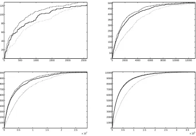
Figure 1 displays the number of items found as a function of time by the Good-UCB (solid), the OCL (dashed) and the uniform sampling scheme that alternates between experts (dotted). The results are presented for sizes N=128,N =500,N =1000 and N =10000, each time for one representative run (averaging over different runs removes the interesting variability of the process). We chose to plot the number of items found rather than the waiting timetas the former is easier to visualize while the latter was easier to analyze. In fact, macroscopic optimality in terms of number of items found could also be derived with the techniques of Section 3. Figure 1 also shows clearly the macroscopic convergence of Good-UCB to the OCL. Moreover, it can be seen that, even for very moderate values ofN, the Good-UCB significantly outperforms uniform sampling even if it is clearly distanced by the OCL.

0 500 1000 1500 2000 2500 0

20 40 60 80 100 120

0 2000 4000 6000 8000 10000 12000 0

50 100 150 200 250 300 350 400 450 500

0 0.5 1 1.5 2 2.5

x 104 0

100 200 300 400 500 600 700 800 900 1000

0 0.5 1 1.5 2 2.5 3 3.5

x 105 0

1000 2000 3000 4000 5000 6000 7000 8000 9000 10000

Figure 1: Number of items found by Good-UCB (solid), the OCL (dashed), and uniform sampling (dotted) as a function of time for sizesN=128,N=500,N=1000 andN=10000 in a 7-experts setting.

0 1 2 3 4 5

x 105 0

200 400 600 800 1000

0 1 2 3 4 5

x 105 0

200 400 600 800 1000

Figure 2: Number of prime numbers found by Good-UCB (solid), the OCL (dashed), and uni-form sampling (dotted) as a function of time, using geometric experts with means 100,300,500,700 and 900, forC=0.1 (left) andC=0.02 (right).

random variables, with expectations 100, 300, 500, 700 and 900 respectively. The set of interest-ing items is the set of prime numbers. We compare the oracle closed-loop policy, Good-UCB and uniform sampling. The results are displayed in Figure 2. Even if the difference remains significant between Good-UCB and the OCL, the former still performs significantly better than uniform sam-pling during the entire discovery process. In this example, choosing a smaller parameterCseems to be preferable; this is due to the fact that the proportion of interesting items on each arm is low; in that case, it may be possible to show, by using tighter concentration inequalities, that the concen-tration of the Good-Turing estimator is actually better than suggested by Proposition 1. In fact, this experiment suggests that the value ofCshould be chosen smaller when the remaining missing mass is small.

Acknowledgments

We are especially thankful to one of the anonymous referees for suggesting to us to write Sec-tions 2.3 and 2.4.

Appendix A.

Proof of lemma 2We proceed by induction ont. Fort=1, the result is obvious. Fort>1, denote by ¯πthe policy choosingI₁π¯ =I₁πand then playing like OCL for thet₋1 remaining rounds. Denote H1= (I₁π,XI₁π,1), andFπ(2 :t)(respectivelyFπ¯(2 :t)) the number of interesting items found by policy

π(respectively ¯π) between rounds 2 andt. Note that conditionally onH1,Fπ¯(2 :t)corresponds to F∗(t₋1) in some modified problem (where one interesting item on expert I₁π might have been removed from the set of interesting items). Thus one can apply the induction hypothesis to obtain

E_[Fπ_{(2 :t)|H1]≤}E

Fπ¯(2 :t)_|H1

.

Let us assume in the following thatI₁πis deterministic (we make this assumption only for sake of clarity, everything go through with a randomized choice ofI₁π). Then thanks to the above inequality one has

E_Fπ_{(t) =RI}π

1,0+E[F

π_{(2 :t)]}

≤RI₁π,0+E

Fπ¯(2 :t)

=E_Fπ¯_{(t). (8)}

Now let

τ=min_{s_≥1 :I_s∗=I₁π_}.

On the eventτ_≤t, OCL and ¯πobserve exactly the same items during thetfirst rounds, and thus

Fπ¯(t)1{τ≤t}=F

∗_(t)

1{τ≤t}. (9)

On the other hand on the eventτ>t, ¯πobserve the same items between rounds 2 andtthan OCL between rounds 1 andt₋1, that isFπ¯(2 :t)1{τ>t}=F

∗_(t−1)

1{τ>t}. Thanks to assumption

(i), this implies (denotingY₁∗, . . . ,Y_t∗for the sequence of items observed by OCL), Fπ¯(t)1{τ>t}= 1{XIπ

1,1∈A}+F ∗_(t)−

1{Y

∗

t ∈A\ {Y1∗, . . . ,Yt∗−1}}

1{τ>t}. (10)

By combining (8), (9) and (10), it only remains to show that

E_[1{XIπ 1,1∈A}

1{τ>t}]≤E[1{Y

∗

SinceXI1π,1is independent of1{τ>t}, one hasE[1{XIπ

1,1∈A}1{τ>t}] =E[RIπ

1,01{τ>t}].

More-over, noting that1{τ>t},I

∗ t andRI∗

t,n∗I_t∗,t−1are measurable with respect toH ∗

t₋1= I1∗,Y1∗, . . . ,It∗₋1,Yt∗₋1

, one has

E_[1{Y

∗

t ∈A\ {Y1∗, . . . ,Yt∗−1}}1{τ>t}] =E[RI∗

t,n∗_I∗

t,t−1

1{τ>t}].

Finally remark that on the eventτ>t one necessarily have that the remaining missing mass on the expert pulled at time t by OCL is larger than the initial missing mass of expert I₁π, that is RIt∗,n∗_I∗

t,t−1

1{τ>t} ≥RIπ 1,0

1{τ>t}, which concludes the proof of (11).

Proof of Lemma 3 Let Y_sπ = XIπ

s,nIsπ,s be the item observed by π at time step s, and

H_sπ= I₁π,Y₁π, . . . ,I_sπ₋₁,Y_sπ₋₁) be the history ofπ prior to making the decision on times. For any

historyhs= (i1,y1, . . . ,is−1,ys−1), letF∗(t|hs)be the number of newly discovered interesting items

when running OCL from the historyhsfort−s+1 steps. ’From the historyhs’ means that, prior to

running OCL, the sequence of expertsi1, . . . ,is−1 has been chosen and has led to the observations y1, . . . ,ys−1. For s′ ≥s we shall also denoteIs∗′(hs) (respectivelyY_s∗′(hs)) the sequence of expert

requests made by OCL starting aths(respectively the corresponding sequence of observed items).

Note in particular that ¯Isdefined in the statement of the lemma corresponds toIs∗(Hsπ). We shall also

needτsto be the first time when OCL, running from historyHsπ, selects expertIsπ, that is

τs=min{s′≥s:Is∗′(H_sπ) =I_sπ},

andτs= +∞if there is no interesting item to be found by expertIsπat times.

We shall prove that

E_[F∗_(t|Hsπ_)−F∗_(t|Hsπ_+1)]≤E_RIs¯,nπ

¯

Is,s−1, (12)

which inductively yields the lemma sinceF∗(t) =F∗(t_|h1)andF∗(t|ht+1) =0.

First let us consider the case when τs≤t. Then the observed items with OCL (running from

H_sπ) between stepsandtremains unchanged if one forces OCL to playI_sπat time steps, that is

F∗(t_|H_sπ)1{τs≤t}=1{Y

π

s ∈A\ {Y1π, . . . ,Ysπ−1}}1{τs≤t}+F

∗_(t|Hπ

s+1)1{τs≤t}.

On the other hand ifτs>t, the behavior of OCL will be the same if played fort−ssteps fromHsπ

or fromH_sπ₊₁, that is

F∗(t₋1_|H_sπ)1{τs>t}=F

∗_(t|Hπ

s+1)1{τs>t}.

Moreover note that

F∗(t₋1_|H_sπ) =F∗(t_|H_sπ)₋1{Y

∗

t (Hsπ)∈A\ {Y1π, . . . ,Ysπ−1,Ys∗(Hsπ), . . . ,Yt∗−1(Hsπ)}}.

Thus we proved so far that

F∗(t|H_sπ)₋F∗(t|H_sπ₊₁) =1{Y

π

s ∈A\ {Y1π, . . . ,Ysπ₋1}}1{τs≤t} +1{Y

∗

t (Hsπ)∈A\ {Y1π, . . . ,Ysπ−1,Ys∗(Hsπ), . . . ,Yt∗−1(Hsπ)}}1{τs>t}

≤1{Y

π

s ∈A\ {Y1π, . . . ,Ysπ−1}}1{τs≤t}+1{Y

∗

Now remark thatY_sπis independent ofτsconditionally toHsπ. Thus one immediately obtains

E_[1{Y

π

s ∈A\ {Y1π, . . . ,Ysπ−1}}1{τs≤t}|H

π

s]

=RIs,nπ_Is,s−1E[1{τs≤t}|H

π

s]

≤RIs¯,nπ_Is¯_,s−1

E_[1{τs≤t}|H

π

s].

SimilarlyY_t∗(H_sπ)is independent of1{τs>t}conditionally to(H

π

s,It∗(Hsπ))and thus

E_[1{Y

∗

t (Hsπ)∈A\ {Y1π, . . . ,Ysπ−1}}1{τs>t}|H

π

s,It∗(Hsπ)]

=E_[RI∗

t(Hsπ),nπ_I∗

t(Hsπ),s−1|H

π

s,It∗(Hsπ)]E[1{τs>t}|H

π

s,It∗(Hsπ)]

≤RIs¯,nπ_Is¯,s−1

E_[1{τs>t}|H

π

s,It∗(Hsπ)].

Putting everything together one obtains (12), which concludes the proof.

Lemma 9 Let a>0, b_≥0.4, and x_≥e, such that x_≤a+blogx. Then one has

x_≤a+blog(2a+4blog(4b)).

Proof Ifa_≥blogxthenx_≤2aand thusx_≤a+blog(2a). On the other hand ifa<blogxthenx_≤ 2blogxwhich easily impliesx_≤4blog(4b)(indeed forx_≥e,x_7→logx_xis increasing and furthermore forb_≥0.4 one can check that 4blog(4b)>2blog(4blog(4b))) and thusx_≤a+blog(4blog(4b)). In any case one hasx_≤a+blog(2a+4blog(4b)).

Lemma 10 For all1_≤k_≤n,

−1_k+logn k ≤

n

∑

j=k+1 1

j ≤log n k .

Proof The standard sum/integral comparison yields

logn+1 k+1 ≤

n

∑

j=k+1 1

j ≤log n k ,

but

logn+1 k+1 =log

n k+log

1+ 1

n+1

−log

1+ 1

k+1

≥logn k+0−

Appendix B. The Open-loop Oracle Policy

In this final section, we provide an macroscopic analysis of the open-loop oracle policy in the case of uniform sampling, that is under Hypotheses (i), (ii) and (iii). An open-loop policy must choose, for each horizont, the respective numbers of requests(nN₁, . . . ,nN_K) for each distribution (so that nN₁+_···+nN_K=tN) in advance. It appears here that, in the limit, theoracle open-loop(OOL) policy, which makes use of the parameters(QN₁, . . . ,QN_K), is as good as the OCL policy.

Let here RN_i,nN i

= (QN_{i −}F_iN(nN_i ))/N be the proportion of interesting items not yet found with

expertiafternN_i requests. Suppose thattN/N_→t, and thatnN_i /N_→νi asN goes to infinity; it is

easily shown that, almost surely,

lim

N→∞R

N i,nN

i =Nlim→∞E

h

RN_i,nN i

i

= lim

N→∞

QN i 1−N1

nNi

N =qiexp(−νi).

Hence, the proportion of interesting items found with the allocation(nN₁, . . . ,nN_K)almost surely con-verges to∑K_i=1qi(1−exp(−νi)). Defining

r(ν) =

K

∑

i=1

qiexp(−νi),

it follows that finding the best macroscopic allocation reduces to the following constrained convex minimization problem:

min

ν∈RKr(ν) such thatν1+···+νK=tand∀i,νi≥0.

The solutionr∗(t), reached atν=ν∗(t), is easily derived by classical optimization techniques:

Proposition 11 For every i_{∈ {}1, . . . ,K_}, let q_i =exp 1/i_×∑ik=1logqk

denotes the geometric mean of q1, . . . ,qi.

1. There exists I(t)_{∈ {}1, . . . ,K_}such that







∀i_≤I(t), ν∗

i(t) =I(tt)+log

qi q

I(t)

∀i>I(t), ν∗_i(t) =0.

Hence,

r∗(t) =I(t)q_I(t)exp

−_I(t_t)

+

_∑

i>I(t) qi.

2. There exists1=t1≤ ··· ≤tK<+∞such that

∀t_∈[ti,ti+1[,I(t) =i.

The(tk)kare such that

qi+ (i−1)q_i−1exp

−_i ti −1

=iq_iexp

−t_ii.

Proof:Introduce the Lagrangian:

L(ν1, . . . ,νK,λ,µ1, . . . ,µK) = K

∑

i=1 qiexp

−ν_Ni+λ

K

∑

i=1

νi

!

−

K

∑

i=1 µiνi.

We need to find the solution of:

∀i_{∈ {}1, . . . ,M_}, ₋qiexp(−νi) +λ−µi=0, K

∑

i=1

νi=t,

∀i_{∈ {}1, . . . ,M_}, µiνi=0 andµi≥0.

We first obtain that

νi=logqi−log(λ−µi).

DenotingA=_{i:νi>0}, and using thati∈A =⇒ µi=0, we get

t=

∑

i∈A

log(qi)− |A|log(λ),

from which we get

−log(λ) = t

|A_|− 1

|A_|i

∑

_∈Alogqi,

and then for alli_∈A:

νi=logqi+

t |A_|−

1

|A_|i

∑

_∈Alogqi.

Next, observe thatνi=0 ⇐⇒ qi>λ: in fact, ifνi=0 then the first equation gives−qi+λ−µi=0,

and 0_≤µi=λ−qi. Conversely, ifνi>0 thenµi=0 andνi=log(qi/λ)>0 impliesqi>λ. Thus,

there existsI(t)such thatA=_{1, . . . ,I(t)_}, and for alli_≤I(t),

νi=log

qi

q_I(t)+ t I(t) .

Moreover,

r∗(t) =r ν1, . . . ,νI(t),0, . . . ,0

=

_∑

i≤I(t) qiexp

"

− log qi q_I(t)+

t I(t)

!#

+

_∑

i>I(t) qi

=I(t)q

I(t)exp

− t I(t)

+

_∑

i>I(t) qi.

The instants(ti)1≤i≤K are such that

(i₋1)q_i

−1exp

−_iti −1

+

∑

k>i−1

qk=iq_iexp

−t_ii+

∑

k>i

which is equivalent to

qi+ (i−1)q_i−1exp

−_iti −1

=iq_iexp

−t_ii.

Fori=2, this gives

0=q2+q1exp(−ν2)−2√q1q2exp

−ν₂2=√q2−

p

q1exp(−ν2)

2

,

which leads tot1=log(q1/q2).

Theorem 12 In the macroscopic limit, the proportion of items found by the open-loop oracle policy uniformly converges to the function F defined in Equation(7).

The proportion of interesting items found by the OOL policy is

q₋r∗(t) =

∑

i≤I(t)

qi−q_I(t)exp

−_I(t_t)

=

K

∑

i=1

(qi−Λ(t))₊ ,

whereΛ(t) =q_I(t)exp

−I(tt)

∈[0,qI(t)]. To conclude, it remains only to remark that Λ=T−1, whereT is defined in Equation (6). In fact, ifλis such thatqi0+1<λ≤qi0, thenI(T(λ)) =i0and

Λ(T(λ)) =q_i

0exp

−T(_iλ) 0

=exp 1

i0_i

∑

_≤i0 logqi

!

exp

−∑i≤i0log(qi/λ)

i0

=λ.

Ifλ<qK, the same holds withi0=K. References

P. Auer, N. Cesa-Bianchi, and P. Fischer. Finite-time analysis of the multiarmed bandit problem. Machine Learning, 47(2):235–256, 2002.

S. Bubeck and N. Cesa-Bianchi. Regret analysis of stochastic and nonstochastic multi-armed bandit problems. Foundations and Trends in Machine Learning, 5(1):1–122, 2012.

F. Fonteneau-Belmudes. Identification of Dangerous Contingencies for Large Scale Power System Security Assessment. PhD thesis, University of Li`ege, 2012.

F. Fonteneau-Belmudes, D. Ernst, C. Druet, P. Panciatici, and L. Wehenkel. Consequence driven decomposition of large-scale power system security analysis. InProceedings of the 2010 IREP Symposium - Bulk Power Systems Dynamics and Control - VIII, Buzios, Rio de Janeiro, Brazil, August 2010.

W.A. Gale and G. Sampson. Good-turing frequency estimation without tears. Journal of Quantita-tive Linguistics, 2(3):217–237, 1995.

I.J. Good. The population frequencies of species and the estimation of population parameters. Biometrika, 40:237–264, 1953. ISSN 0006-3444.

D. McAllester and L. Ortiz. Concentration inequalities for the missing mass and for histogram rule error. J. Mach. Learn. Res., 4:895–911, December 2003. ISSN 1532-4435.

D.A. McAllester and R.E. Schapire. On the convergence rate of Good-Turing estimators. InCOLT, pages 1–6, 2000.

C. McDiarmid. On the method of bounded differences. InSurveys in combinatorics, 1989 (Norwich, 1989), volume 141 ofLondon Math. Soc. Lecture Note Ser., pages 148–188. Cambridge Univ. Press, Cambridge, 1989.