Classification of Imbalanced Data with a Geometric Digraph
Family
Art¨ur Manukyan [email protected]
Graduate School of Sciences and Engineering Ko¸c University
Sarıyer, 34450, Istanbul, Turkey
Elvan Ceyhan [email protected]
Department of Statistics University of Pittsburgh Pittsburgh, 15260, PA, USA
Editor:William Cohen
Abstract
We use a geometric digraph family called class cover catch digraphs (CCCDs) to tackle the class imbalance problem in statistical classification. CCCDs provide graph theoretic solutions to the class cover problem and have been employed in classification. We assess the classification performance of CCCD classifiers by extensive Monte Carlo simulations, comparing them with other classifiers commonly used in the literature. In particular, we show that CCCD classifiers perform relatively well when one class is more frequent than
the other in a two-class setting, an example of theclass imbalance problem. We also point
out the relationship between class imbalance and class overlapping problems, and their influence on the performance of CCCD classifiers and other classification methods as well as some state-of-the-art algorithms which are robust to class imbalance by construction. Experiments on both simulated and real data sets indicate that CCCD classifiers are robust to the class imbalance problem. CCCDs substantially undersample from the majority class while preserving the information on the discarded points during the undersampling pro-cess. Many state-of-the-art methods, however, keep this information by means of ensemble classifiers, but CCCDs yield only a single classifier with the same property, making it both appealing and fast.
Keywords: Class Cover Catch Digraphs, Class Cover Problem, Class Imbalance Problem, Class Overlapping Problem, Graph Domination, Prototype Selection, Support Estimation
1. Introduction
Class imbalance problem has recently become a topic of extensive research. In a two-class setting, imbalance in class(es) occurs when one class is represented by far more observations
(points) than the other class in the data set (see, e.g., Chawla et al. (2004) and L´opez
mostly the ones who have fair results are kept (Thai-Nghe et al., 2009). In these and many other real life cases, majority class (i.e., the class with larger size) confounds the classifier performance by hindering the detection of subjects from the minority class (i.e., the class with fewer points).
The classification methods in machine learning usually suffer from the imbalance of class sizes in the data sets because most of these methods work on the assumption that class sizes
are balanced (Japkowicz and Stephen, 2002). For example, the commonly used k-nearest
neighbor (k-NN) classification algorithm is highly influenced by the class imbalance problem.
In the k-NN approach, a new point is classified as the class of the most frequent one from
its firstknearest neighbors (Fix and Hodges, 1989; Cover and Hart, 1967). As a result, in a
two-class setting where one class substantially outnumbers the other, a point is more likely
to be classified as the majority class by thek-NN classifier. In literature, sensitivity ofk-NN
classifier to the class imbalance problem and some solutions on choosing the appropriatek
have been discussed in cases of imbalanced classes (see Mani and Zhang, 2003; Garc´ıa et al., 2008; Hand and Vinciotti, 2003). Decision trees and support vector machines (SVM) are also some of the well known classifiers that are sensitive to the class imbalance in a data set (Japkowicz and Stephen, 2002; Tang et al., 2009). SVMs are among the most commonly used algorithms in the machine learning literature due to their well understood theory and high
performance among popular algorithms (Wu et al., 2008; Fern´andez-Delgado et al., 2014),
but these methods have been demonstrated to be inefficient against highly imbalanced data sets, although SVMs are still robust to moderately imbalanced data sets (Akbani et al., 2004; Raskutti and Kowalczyk, 2004).
We approach the classification of imbalanced data sets with methods that solve class cover problem (CCP), where the goal is to find a region that encapsulates all the members
of the class of interest (i.e., target class). This particular region can be viewed as a cover;
hence the name class cover (Cannon and Cowen, 2004). This problem is closely related
to another problem in statistics, namely support estimation: estimating the support of a
particular random variable defined in a measurable space (Sch¨olkopf et al., 2001). Here,
In this article, we study the effects of class imbalance on two CCCD classifiers, P-CCCD and RW-P-CCCD. Moreover, we report on the effects of class overlapping problem (which is defined as deterioration of classification performance when class supports overlap) along with the class imbalance problem to further investigate the performance of CCCD classifiers when imbalance and overlapping between classes co-exist. Thus, we show that when there is a considerable amount of class imbalance, whether class supports overlap or
not, the CCCD classifiers perform better than thek-NN classifier. We show the robustness of
CCCD classifiers to the class imbalance by simulating cases having increasing levels of class imbalance. We also compare CCCD classifiers with SVM classifiers which are potentially robust to moderate levels of class imbalance but not to high levels. With respect to class
imbalance problem, the k-NN, SVM and decision tree classifiers may be referred to as
“weak” classifiers; that is, these methods perform weakly when there is imbalance in the data set. However, such classifiers can be modified to address the unequal priors in a data set, and hence, can be converted to “strong” classifiers which are potentially robust to the class imbalance problem. We show that CCCD classifiers are also inherently robust (i.e., robust to class imbalance without any modification), and we compare the CCCD classifiers against the state-of-the-art strong classification methods which are constructed to perform well when class imbalance occurs. We consider ensemble learning, cost sensitive learning
and resampling schemes in conjunction with k-NN, SVM and decision tree classifiers, and
show that RW-CCCDs and P-CCCDs perform comparable to those strong classifiers.
Among the two variations of CCCD classifiers, we show that the RW-CCCD is more appealing in many aspects. For both simulated and real life examples, RW-CCCDs perform better than P-CCCDs and weak classifiers, and perform comparable to strong classifiers when the classes of data sets are imbalanced and/or overlapping. Moreover, we report on the complexity of the two CCCD classifiers and demonstrate that RW-CCCDs reduce the data sets substantially more than the other classifiers, thus increasing the testing speed. But most importantly, while reducing the majority class to mitigate the effects of class imbalances, CCCDs preserve the information on the discarded points of the majority class. CCCDs provide a novel potential solution to the class imbalance problem; that is, they capture the density around prototype points (i.e., members of the dominating sets) as radii of the covering balls. Hence, CCCDs preserve the information while reducing the data set In the literature, only the strong classifiers based on hybrids of ensembles and resampling schemes achieve a similar task which requires multiple classifiers to be employed, and thus, result in lengthy training and testing time. However, CCCDs define single classifiers that undersample the data set with, possibly, a slight loss of information.
2. Methods for Handling Class Imbalance Problem
Solving the class imbalance problem received considerable attention in the machine learning literature (see Chawla et al., 2004; Kotsiantis et al., 2006; Longadge and Dongre, 2013). Almost all algorithms designed to mitigate the effects of class imbalance incorporate a “weak” classifier which is modified to show some level of robustness to the class imbalance problem. The weak algorithm is modified either (i) in data level which involves a pre-processing of the data set being used in training, or (ii) in algorithmic level such that a “strong” classifier is constructed with a decision rule suited for the imbalances in the data set. Many modern algorithms are hybrids of both types; but in particular, there are mainly three of them: resampling methods, cost-sensitive methods, and ensemble methods (He and Garcia, 2009).
Resampling methods are commonly employed to remove the effects of class imbalance in the classification process. Resampling methods provide solutions to the class imbal-ance problem by (i) downsizing the majority class (undersampling) or (ii) generating new (synthetic) points for the minority class (oversampling). Hence, such methods modify the classifiers only at the data level. It might be useful to clean or erase some points in the ma-jority class to balance the data (Drummond et al., 2003; Liu et al., 2009). However, in some cases, all points from both classes may be valuable/important, and hence, should be kept despite the differences in the class sizes. Oversampling methods generate synthetic points similar to the minority class to mitigate the class imbalance problem while preserving the information (Han et al., 2005). On the other hand, Batista et al. (2004) suggest that the combination of both over and undersampling methods can further improve the classifica-tion performance. One such method is the SMOTE+ENN method where the oversampling method SMOTE of Chawla et al. (2002) and edited nearest neighbors (ENN) method of Wilson (1972) are applied to an imbalanced data set, consecutively. While SMOTE bal-ances the classes of the data set by generating artificial points between members of the minority class, ENN cleans the data set to further increase the classification performance of the weak classifier. Here, ENN method is an undersampling method that primarily aims to remove noisy points from the data set but not to balance the classes.
Another family of methods, namely cost-sensitive learning methods, has originated from real life: the cost of misclassifying a minority and a majority class member is usually not the same (Elkan, 2001). Frequently, the minority class has higher misclassification cost than the majority class. Classification methods such as decision trees (e.g., C4.5), can be modified to take these costs into account (see Ling et al., 2004; Zadrozny et al., 2003). C5.0 is an extended version of C4.5 incorporating the cost of each class (Kuhn and Johnson, 2013). Most weak classifiers can be easily modified so as to recognizing misclassification
costs. The constrained violation cost C of SVM classifiers can be adjusted to individual
class costs (Chang and Lin, 2011). As for k-NN, one solution is to appoint weights to all
A fast developing field called ensemble learning also contributes to the family of methods handling the class imbalance problem (see Galar et al., 2012). The idea is to combine several classifiers to create a new classifier which has significantly better performance than its constituents (Rokach, 2010). AdaBoost is a popular algorithm among this family of learning methods (Freund and Schapire, 1997; Wu et al., 2008). AdaBoost assigns weights to each of the points in the data set and updates these weights in accordance with how well the points are estimated by each classifier. Galar et al. (2012) provide a survey of the most important ensemble learning methods that solve the class imbalance problem. However, it has been observed in some studies that ensemble learning methods work best
when used together with resampling methods (L´opez et al., 2013). In fact, ensembling and
resampling schemes compensate the shortcomings of each other. The EasyEnsemble is a classifier with two levels of ensembles. First, a random undersampled majority class and the original minority class are used to train an ensemble classifier, then another random sample is drawn in the same way to train a second ensemble. This process is repeated several times to mitigate the effects of information loss as each ensemble would be applied on a different random subset of the majority class.
3. Classification with Class Cover Catch Digraphs
Class Cover Catch Digraphs (CCCDs) offer graph theoretic solutions to CCP (Priebe et al., 2001, 2003a). The objective of CCP is to find a region that covers the members of a specific
class. More specifically, let (Ω, M) be a measurable space and letXn = {x1, x2, ..., xn} ⊂
Ω and Ym = {y1, y2, ..., ym} ⊂ Ω be observations from two classes X and Y with class
conditional distributions FX, FY and a joint cdf FX,Y, respectively. Let Ω = Rd and,
without loss of generality, assume that the target class (i.e., the class of interest) is X. In
a CCCD, for xi, xj ∈ Xn ⊂ Rd is the center of a ball with radius ri =r(xi). Each ball is
represented by Bi = B(xi, ri) and ifxj ∈ Bi then xi is said to cover (or catch)xj. Here,
d(., .) can be any dissimilarity measure but we use the Euclidean distance henceforth. A
CCCD is a digraph D=D(V, A) with vertex set V(D) =Xn and the arc setA(D) where
(xi, xj)∈A(D) if and only ifxj ∈Bi. The term “catch” refers to arc (xi, xj) of the digraph
D where xi is said to catch xj. The binary relation xi ∼xj, which is defined as xj ∈ Bi,
is asymmetric, thus the adjacency of xi and xj is represented with directed edges or arcs
which yield a digraph instead of a graph.
In CCCDs, the goal is to find a subset of balls CX ⊆BX ={B1, B2, ..., Bn} such that
QX ⊆ ∪B∈CXB forQX ⊆ Xn where the setQX is some desirable subset of the target class
training set Xn which we want to cover. Preferably, the goal is to find a set CX such that
QX =Xn, however it might be desirable that the class cover may ignore some target class
points to avoid overfitting. If a class cover of a CCCD fails to cover some target class points,
it is called animproper cover, otherwise it is apropercover. For coveringYm, we reverse the
roles of classesX andY. The classYbecomes the target class andX becomes the non-target
class. Finding an appropriate cover CX is equivalent to finding the dominating set of the
CCCD with V(D) =Xn. Let N(s) ={t∈V(D) : (s, t)∈A(D)}be the open neighborhood
of a vertexs∈V(D): the set of vertices that have an arc from the vertexs, or the neighbors
of s. A dominating set of a digraph D is defined as a subset of vertices S ⊆ V(D) such
is the vertex set of the digraph: ∪s∈SN¯(s) = V(D). Among all dominating sets, usually
the ones with minimum cardinality, called the minimum dominating sets, are preferable.
The cardinality of the minimum dominating set(s) is referred to as thedomination number,
denoted asγ(D). However, minimum dominating sets are often computationally intractable
and finding them is, in general, an NP-hard optimization problem. Hence, greedy algorithms are often employed to find sets with approximately minimum cardinality (Chvatal, 1979; DeVinney, 2003).
CCCDs can easily be generalized to the multi-class case withkclasses. To establish the
set of covers C = {C1, C2,· · ·, Ck} associated with a set of classes X = {X1,X2,· · · ,Xk},
we merge the classes into two classes as XT = Xi and XN T = ∪i6=jXj for i, j = 1,· · ·, k.
We refer to classes XT and XN T as target class and non-target class, respectively. More
specifically, target class is the class we want to find the cover of, and the non-target class is the union of the remaining classes. We transform the multi-class case into a two-class
setting and find the cover ofi-th class,Ci, for each i= 1,· · ·, k.
We employ two families of CCCDs, pure-CCCDs (P-CCCDs) and random walk CCCDs
(RW-CCCDs) that differ in the definition of the radius r(x). In these two digraphs, the
(approximate) minimum dominating setS and the classifier are defined in slightly different
ways; with the main distinction between the two being the way the covers are defined. The covering balls of P-CCCDs do not contain any non-target class point (hence the name “pure”) whereas RW-CCCDs possibly allow some non-target class points inside of the class cover of the target class so as to avoid overfitting. Moreover, some target class points may also be excluded from the covers of RW-CCCDs. Therefore, P-CCCDs construct pure and proper covers but RW-CCCD covers are not necessarily pure or proper.
3.1 Classification with P-CCCDs
In P-CCCDs, the covering ballsBx =B(x, r(x)) exclude all non-target class points. Thus,
for a target class point x ∈ Xn, which is the center of a ball Bx, the radius r(x) should
be smaller than the distance between x and the closest non-target point y ∈ Ym: r(x) <
miny∈Ymd(x, y). Given τ ∈(0,1], the radius r(x) is defined as follows (Marchette, 2010):
r(x) := (1−τ)d(x, l(x)) +τ d(x, u(x)), (1)
where
u(x) := argmin
y∈Ym
d(x, y)
and
l(x) := argmax
z∈Xn
{d(x, z) :d(x, z)< d(x, u(x))}.
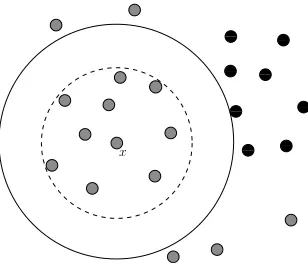
The effect of parameterτ on the radiusr(x) is illustrated in Figure 1 (DeVinney, 2003).
The ball with radiusr(x) catches the neighboring target class points, and for anyτ ∈(0,1],
the ball Bx catches the same points as well. Hence, the choice of τ does not effect the
structure of digraph but might affect the classification performance which will be shown
later in Section 5. On the other hand, for allx∈ Xn, the definition ofr(x) in Equation (1)
keeps any non-target pointy ∈ Ym out of the ballBx, that isYm∪Bx =∅for allBx ∈CX.
00 00 00 11 11 11
00 00 00 11 11 11 000 000 000 111 111 111
00 00 00 11 11 11
00 00 00 11 11 11
000 000 000 111 111 111
00 00 00 11 11 11 00 00 00 11 11 11
x
Figure 1: The effect ofτ on the radiusr(x) of the target class pointxin a two-class setting.
Grey and black points represent the target and non-target classes, respectively.
The solid circle centered atxis constructed with the radius associated withτ = 1
and the dashed one withτ = 0.0001 (DeVinney, 2003).
the balls contain only the target class points; hence, the name pure-CCCD. Once all balls
are constructed, so is the digraph D. Therefore, we have to find a covering setCX which
is equivalent to finding a minimum dominating set S ⊆ V(D). The greedy algorithm of
finding an approximate minimum dominating set of a P-CCCD is given in Algorithm 1. At each iteration, the vertex which has the largest neighborhood (i.e., highest number of arcs) is removed from the graph together with its neighbors. Then, the process is repeated until
all vertices of Dare removed. The algorithm adds elements to the dominating set until all
points are either dominated or dominate some other points. Hence, the covers established
by P-CCCDs are proper covers: QX = Xn and QY =Ym. The P-CCCD of one class, its
associated class cover (constructed by the elements of the dominating set), and covers of both classes are illustrated in Figure 2.
Algorithm 1 The greedy algorithm for finding an approximate minimum dominating set
of a digraph D. Here, D[H] is the graph induced by the set of vertices H ⊆ V(D) (see
West, 2000).
Input: A digraphD=D(V, A)
Output: An approximate minimum dominating set,S
1: set H =V(D) andS=∅
2: while H 6=∅ do
3: v∗= argmaxv∈V(D)|N¯(v)|
4: S=S∪ {v∗}
5: H =V(D)\N¯(v∗) 6: D=D[H]
7: end while
Before Algorithm 1 finds an approximate solution, we should first construct the digraph
D. The P-CCCD cover CX and the P-CCCD D depend on the distances between points
of the target class Xn, denoted by the matrix MX, and the distances from all points of
BX = {B1, B2, ..., Bn}, and get the set of arcs A(D) where V(D) = Xn. Hence, the
minimum cardinality ball cover problem is reduced to a minimum dominating set problem. We find such a cover with Algorithm 2 which runs in quadratic time and, in addition,
depends on the dimensionality of the training set Xn∪ Ym.
Algorithm 2The greedy algorithm for finding an approximate minimum cardinality ball
coverCX of the target class points Xn given a set of non-target class pointsYm.
Input: Points of the target classXn, the non-target classYmand the P-CCCD parameterτ∈(0,1]
Output: An approximate minimum cardinality ball coverCX
1: r(x) := (1−τ)d(x, l(x)) +τ d(x, u(x)) for allx∈ Xn
2: Construct the digraph D with the setBX.
3: Find the approximate minimum dominating setS of digraphD by Algorithm 1.
4: CX :=∪s∈SB(s, r(s))
Theorem 1Algorithm 2 is an O(logn)-approximation algorithm and finds an approximate
minimum cardinality ball coverCX of the target class X in O(n(n+m)d) time.
Proof. The algorithm is polynomial time reducible to a greedy minimum set cover algorithm
which finds an approximate solution with size at most O(logn) times of the optimum
solution (Chvatal, 1979; Cannon and Cowen, 2004). We first calculate the distance matrices
MX andMX Ywhich takeO(n2d) andO(nmd) time, respectively. Constructing the digraph
D requires computing l(x) and u(x) in Equation (1) for all x ∈ Xn, taking O(n2+nm)
time in total. Then, we set the arc set A(D) inO(n2) time. Finally, the algorithm finds a
solution for the digraphD inO(n2) time, hence the total running time of the algorithm is
O(n(n+m)d).
When Y is the target class, observe that the time complexity isO(m(n+m)d), and an
approximate solution is of size at mostO(logm) times the optimal solution by Theorem 1,
since m =|Ym|. A P-CCCD classifier consists of the covers of all classes, hence the total
training time of finding CCCDs of a data set with two-class setting isO((n+m)2d).
After establishing both class covers CX and CY, any new data point can be classified
in Rd according to where it resides. Here, there are three cases according to the location
of the given point, z, to be classified: z is (i) only in CX or CY, (ii) in both CX and CY
or (iii) in neither of CX and CY. The case (i) is straightforward: z belongs to class X if
z∈CX \CY or to class Y ifz∈CY \CX. For cases (ii) and (iii), we need to find a way to
decide the class of the point in a reasonable way. In fact, for all the cases, the estimated
class of a given pointz is determined by
argmin
C∈{CX,CY}
min
x:B(x,r)∈Cρ(z, x)
(2)
whereρ(z, x) =d(z, x)/r(x) (Marchette, 2010). The dissimilarity measureρ(x, z) indicates
whether or not the point z is in the ball of radius r(x) with center x, since ρ(x, z) ≤1 if
z is inside the (closure of the) ball and > 1 otherwise. The measure ρ : Ω×Ω → R+ is
simply a scaled dissimilarity measure, since Euclidean distance between two points,d(x, y),
is divided (or scaled) with the radius, r(x) or r(y). This measure violates the symmetry
axiom among metric axioms sinceρ(x, y)6=ρ(y, x) whenever r(x)6=r(y). However, Priebe
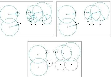
Figure 2: An illustration of the CCCDs (with the grey points representing the points from the target class) in a two-class setting. Presented in top left are all covering balls
and the digraph D= (V, A) and in top right are he balls that constitute a class
cover for the target class and are centered at points which are the elements of the
dominating setS⊆V(D). In the bottom panel, we present the dominating sets
of both classes and their associated balls which establish the class covers. The class cover of grey points is the union of solid circles, and that of black points is the union of dashed circles.
i.e., under the assumptions that both FX and FY are continuous and strictly separable
(infx∈Xn,y∈Ymd(x, y) =δ >0), P-CCCD classifiers are consistent; that is, their
misclassifi-cation error approaches to the Bayes optimal classifimisclassifi-cation error asm, n→ ∞. The measure
ρ favors points with bigger radii; that is, for example, for a new pointz equidistant to two
points, the point with bigger radius is closer in terms of this scaled dissimilarity measure;
for example,ρ(x, z) < ρ(y, z) when d(x, z) =d(y, z) and r(x) > r(y). The radius r(x) can
be viewed as an indicator of the density around the point x. Thus, a point x with bigger
radius might suggest that the point z is more likely be drawn from the same distribution
(or class) wherex is drawn (i.e., from the denser class).
3.2 Classification with Random Walk CCCDs
For P-CCCDs, the class covers defined by CCCDs were “pure” of non-target class points; that is, no member of the non-target class was allowed inside the cover of the target class.
As in Figure 1, the ball centered at the pointxcannot expand any further since its radius is
cover to overfit or be sensitive to noise or outliers in the non-target class. By allowing some neighboring non-target class points inside the cover and some target class points outside the cover, the random walk CCCDs (RW-CCCDs) catch as much target class points as possible
with an adaptive strategy of choosing the radii (DeVinney et al., 2002). For x ∈ Xn,
|Xn|=nand |Ym|=m, RW-CCCDs define a function on radius of a ball given by
Rx(r) =Rx(r;Xn,Ym)
:= m
n|{z∈ Xn:d(x, z)≤r}| − |{z∈ Ym:d(x, z)≤r}|.
(3)
where second and third arguments inRx(r;Xn,Ym) are suppressed when there is no
ambi-guity. The functionRx(r) can be viewed as a one-dimensional random walk. When the ball
centered at x ∈Rd expands, it hits either a target class point or a non-target class point
which increases or decreases the random walk by one unit, respectively. The ratio m/n is
included in the first term as to avoid the bias resulted by unequal sample sizes (i.e., class
imbalance). An illustration is given in Figure 3 for the case m = n. The function Rx(r)
aims to find such radii that it contains a few non-target class points and sufficiently many target class points. In addition, we also want to avoid balls with large radii. Hence, the
radius of xis the value maximizing Rx(r) with an additional penalty functionPx(r) which
biases toward small radii:
rx := argmax
r∈{d(x,z):z∈Xn∪Ym}
Rx(r)−Px(r). (4)
Although a penalty function seems fit, DeVinney (2003) pointed out that the choice of
Px(r) = 0 usually works sufficiently well in practice. As in P-CCCDs, the radius of a
ball represents the density of its center’s neighborhood. Maximizing Rx(r) determines the
best possible radius. Moreover, unlike P-CCCDs, the balls of RW-CCCDs are closed balls:
Bx ={z∈Rd:d(x, z)≤r(x)}.
Similar to P-CCCDs, finding a cover, or a dominating set, of a RW-CCCD is an NP-hard problem. However, RW-CCCDs find the minimum dominating sets in a slightly different
fashion. Instead of finding a setS such that∪s∈SN¯(s) =V(D) as in Algorithm 1, we first
locate the vertex x∗ (a target class point) which has maximum of some score, Tx∗, and
remove all target and non-target class points covered with the ball of this vertex, Bx∗. In
the next iteration, we recalculate the radii of remaining target class points, find the next point with the maximum score and continue until all target class points are covered. This
greedy method of finding dominating set(s) S of RW-CCCDs is given in Algorithm 3. The
resulting dominating set S has approximate minimum cardinality. For each target class
point x∈ Xn, the scoreTx is associated with Rx(rx) and is given by
Tx=Rx(rx)−
rxnu
2dm(x)
(5)
wherenuis the number of uncovered target class points in the current iteration, anddm(x) =
maxz∈Xnd(x, z). The term which is linear in rx of the right hand side of Equation (5) is
similar to P(r) in Equation (4): it biases the scores toward choosing dominating points
with smaller radii. On the other hand, Algorithm 3 is likely to choose dominating points
000 000 000 000
111 111 111 111 00 00 00 11 11 11
00 00 00 11 11 11
r
x Rx
(
r
)
000 000 000 000
111 111 111 111 00 00 00 11 11 11
00 00 00 11 11 11
r
x Rx
(
r
)
Figure 3: Two snapshots of Rx(r) associated with the ballBx centered atx form=n.
Algorithm 3 The greedy algorithm for finding an approximate minimum dominating set
for RW-CCCDs of pointsXn from the target class given non-target class points Ym.
Input: Target class pointsXn and non-target class pointsYm
Output: Approximate dominating setS of Xn
1: H0=Xn,H1=Ym andS=∅
2: ∀x∈ Xn,dm(x) = maxz∈Xnd(x, z)
3: while H06=∅do
4: nu=|H0|
5: for allx∈ Xn do
6: r(x) = argmaxrRx(r;H0, H1) forr∈ {d(x, z) :z∈H0∪H1}
7: end for
8: x∗= argmax
x∈H0Rx(r(x);H0, H1)− r(x)nu
2dm(x)
9: S=S∪ {x∗}
10: H0=H0\( ¯N(x∗)∩ Xn) andH1=H1\( ¯N(x∗)∩ Ym)
11: end while
12: CX :=∪s∈SB(s, r(s))
not covered since their balls have radii r= 0. Hence, RW-CCCDs may establish improper
covers.
Algorithm 3 is similar to Algorithm 2, however after each iteration, a point is added to
the set S and the random walk Rx(r) is recalculated for all uncoveredx ∈A0. Hence, we
need an additional sweep on the training set which makes Algorithm 3 run in cubic time.
Theorem 2 Algorithm 3 finds covers CX of the target class X and Y in O((n+d+
log (n+m))(n+m)2) time.
Proof. In Algorithm 3, the matrix of distances between points of training set Xn∪ Ym
should be computed since, for all x ∈ Xn∪ Ym, the entire data set is swept to maximize
are covered, but for each iteration, the random walk Rx(r) is recalculated. The maximum
Rx(rx) could be found by sorting the distances for all x ∈ A0 which could be done prior
to the while loop. This sorting takes O((n+m)2log (n+m)) time. Since A0 and A1 are
updated at each iteration, we can just erase the distances corresponding to points covered
by ¯N(x∗) which does not change the order of sorted list provided before the while loop.
Hence, argmaxRx(rx) is found and the covered points erased in O((n+m)2) time. The
while loop iterates n times in the worst case, and hence the algorithm runs in a total of
O((n+d+ log (n+m))(n+m)2) time.
Note that Algorithm 3 finds a cover ofYminO((m+d+log (n+m))(n+m)2) time which
makes a RW-CCCD classifier trained in O((n+m)3) time for d < n and log (n+m) < n.
RW-CCCD classifiers are much better classifiers that potentially avoid overfitting, but with a cost of being much slower compared to the P-CCCD classifiers.
Since P-CCCD covers are pure and proper covers, P-CCCD classifiers tend to overfit
(DeVinney, 2003). In RW-CCCDs, covering balls allow some points of Ym inside CX to
increase average classification performance. In that case, Algorithm 3 cannot be reduced to a minimum set cover problem since the definition of sets change after adding a single
point to the dominating set. Hence, the upper bound O(logn) does not apply to
RW-CCCDs. However, we expect to get bigger balls in RW-CCCDs compared the ones in P-CCCDs which intuitively suggests that the covers of RW-CCCDs are lower in cardinality. We conduct empirical studies to show that RW-CCCDs, in fact, produce dominating sets with lower size compared to P-CCCDs in some cases.
In RW-CCCD, once the class covers (or dominating sets) are determined, the scaled dissimilarity measure in Equation (2) is a good choice for estimating the class of a new
point z. However, DeVinney (2003) incorporates the scores of each ball to produce better
performing class covers in classification. Hence, the class of a new pointz is determined by
argmin
C∈{CX,CY}
min
x:B(x,r)∈Cρ(z, x) Te
x
whereρ(z, x) is defined as in Equation (2). Here,e∈[0,1] controls at what level the score
Tx is incorporated. We observe that for d(z, x) < r(x), ρ(z, x) = d(z, x)/r(x) decreases
as Tx increases. Hence, if a new point z is in both covers, z ∈ CX ∩CY, the score Tx
is a good indicator to which class the new point z belongs since the bigger the Tx, the
more likely the ball contains more target class points. For e= 1, we fully incorporate each
scoreTx of covering balls and with e= 0, we ignore the scores. By introducing a value for
the parameter e in (0,1), it is possible to further improve the performance of RW-CCCD
classifiers.
4. Balancing the Class Sizes with CCCDs
number of target class points, and hence substantially reduce the data set (in particular, majority class points). Points of the minimum dominating set correspond to the centers of
balls that establish the class covers. Hence CCCD classifiers can also be viewed asprototype
selection methods where the objective is findind a set of points, or prototypes, S; from
the training set to preserve or increase the classification performance while substantially reducing the sample size. However, the radii of dominating set(s) are also stored and used in the classification process.
In Figure 4, we illustrate the behavior of balls associated with P-CCCDs and RW-CCCDs. Note that in both families of digraphs, balls of the majority class tend to be larger and hence are more likely to catch more majority class points. Since the majority class has much more members than the minority class, balls of the majority points are more likely to catch the neighboring majority points. CCCD classifiers keep the information of ball centers and their associated radii. Larger cardinality of the majority class allows the construction of bigger balls and hence, larger values of radii are more likely to correspond to larger number of catched class members. As a result, CCCDs balance the data set and, at the same time, preserve the information of the local density by retaining the radii. The data set becomes balanced since the center of balls are the points of the new training data set which will be employed later in classification.
The loss of information in undersampling schemes are of course inevitable, however it is possible to preserve a portion of that discarded information by other means. EasyEnsemble is an ensemble classifier used for that very purpose; however, it needs multiple classifiers to be employed. Each classifier is trained on a different balanced subset of the original training data set, and hence the ensemble classifier preserves the information on the entire data set given by a collection of unbiased classifiers. On the other hand, CCCDs achieve the same goal by transforming the density around points into the radii. CCCDs resemble cluster based resampling methods in that regard. Instead of randomly sampling the data set, cluster based sampling schemes divide each class into clusters, and then, oversample the minority class or undersample the majority class proportional to each subclass. Covering balls of CCCDs have a similar purpose which has also been discussed in Priebe et al. (2003b). They use the covering balls of the minimum dominating sets to explore the latent subclasses of each class of gene expression data sets. In fact, the balls of CCCDs may correspond to clusters. Hence, sets of points associated with each cluster is undersampled to a single point (i.e., a prototype or a dominating point), and the information on the cluster is provided by the radius which represents the density of that cluster. The bigger the radius, the more influence a prototype has over the domain. In P-CCCDs, the radii may be sensitive to noise, but RW-CCCDs ignore noisy points to avoid overfitting. Moreover, in RW-CCCDs, we have an additional statistic provided by each cluster, the score given in Equation (5) based on the random walk. We use both the radii and these scores to define the RW-CCCD classifiers, and thus achieve better performing classifiers with more reduction and less information loss. We approach the problem of class imbalance from the perspective of class overlapping problem as well. Several researchers on class imbalance revealed that overlap between the class supports degrade the classification performance of imbalanced data sets even more
(see Prati et al., 2004; Batista et al., 2004, 2005; Galar et al., 2012). Let E ⊂ Rd, and
let s(FX) and s(FY) be the supports of the classes X and Y, respectively. We define E
Figure 4: An illustration of the covering balls associated with majority and minority
P-CCCD (left) and the corresponding RW-P-CCCDs (τ = 0.0001) (right) of an
im-balanced data set in a two-class setting where majority and minority class points are represented by grey dots and black triangles, respectively.
q(E) :=|Ym∩E|/|Xn∩E| be ratio of class sizes restricted to the region E ⊂Rd. We say
q(E) is the “local” imbalance ratio with respect toE. Also, let the “global” imbalance ratio
beq=q(Rd) =m/n. Throughout this work, in both simulated and real data examples, we
study and discuss the local imbalance ratioq(E) restricted to the overlapping regionE and
the global imbalance ratioq. We specifically illustrate the performance of several classifiers
for various levels of class imbalance (local or global) and class overlapping, and assess the
performance of CCCD classifiers compared to weak and strong versions ofk-NN, SVM and
C4.5 classifiers.
5. Comparing CCCDs with Other Classifiers
We study the performance of CCCD classifiers in comparison with weak and strong classi-fiers in two separate sections. Recall that we call a classifier as “weak” when the method is inherently sensitive to class imbalance, and as “strong” when it is non-sensitive (or less sensitive). We use the area under curve (AUC) measure to evaluate the performance of the
classifiers on the imbalanced data sets (L´opez et al., 2013). AUC measure is often used on
5.1 Monte Carlo Simulation Study with Weak Classifiers
In this section, we compare the CCCD-based classifiers, namely P-CCCD and RW-CCCD,
with k-NN, support vector machines (SVM) and C4.5, on simulated data sets. These
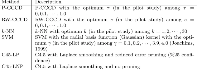
classifiers are listed in Table 1. We employ the cccd, e0171 and RWeka packages in R to
classify test data sets with the P-CCCD, SVM (with Gaussian kernel) and C4.5 classifiers, respectively (Marchette, 2013; Meyer et al., 2014; R Core Team, 2015).
For each of four classification methods other than C4.5, we assign the optimum param-eter values which are the best performing values among all considered paramparam-eters. For
example, an optimum the P-CCCD parameter τ is found in a preliminary (pilot) Monte
Carlo simulation study associated with the main simulation setting (i.e., the same set-ting of the main simulation). In the pilot study, we perform a Monte Carlo simulation
with 200 replications and count how many times aτ value has the maximum AUC among
τ = 0.0,0.1,· · · ,1.0 in 200 trials. Note that, since τ ∈ (0,1], we denote τ = (machine
epsilon) asτ = 0 for the sake of simplicity. For each replication of the pilot simulation, we
(i) classify the test data set with allτ values, (ii) record theτ values with maximum AUC
and (iii) update the count of the recordedτ values. Finally, we appoint the one that has the
maximum count (the best performingτ) as the τ∗, the optimumτ. Then, we useτ∗ as the
parameter of P-CCCD classifier in our main simulation. The parameters of optimalk-NN,
SVM and RW-CCCD classifiers are defined similarly. SVM methods often incorporate both
a kernel parameter γ and a constrained violation cost C. We only optimize γ since the
selection of an optimumC parameter will be more crucial for cost-sensitive SVM methods.
Moreover, we consider two versions of the C4.5 classifier where both incorporate Laplace smoothing. The first tree classifier, C45-LP, prunes the decision tree with %25 confidence level but the second classifier, C45-LNP, does not use pruning at all.
We first consider a simulation setting similar to the one in DeVinney et al. (2002) where
CCCD classifiers showed relatively good performance compared to thek-NN classifier. Here,
we simulate a two-class setting where observations from both classes are drawn from separate
multivariate uniform distributions: FX =U(0,1)d and FY =U(0.3,0.7)d ford= 2,3,5,10.
Notice that s(FY) ⊂s(FX); i.e., E =s(FY). We perform Monte Carlo replications where
on each replication, we train the data with equal sizes of observations (m =n) from each
class for n = 50,100,200,500. On each replication, we record the AUC measures of the
classifiers on the test data set with 100 observations from each class, resulting a test data set of size 200. We simulate test data sets until AUCs of all classifiers achieve a standard error below 0.0005. Average of AUCs of all classifiers in Table 1 are given in Figure 5 for all
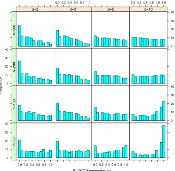
(n, d) combinations. Additionally, in Figure 6, we report theτ values of best performing
P-CCCD classifiers in our pilot simulation study for all (n, d) combinations. In Figure 6, there
are separate histograms for each combination. Each histogram represents the number of
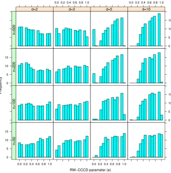
times aτ value has the maximum AUC. Also in Figure 7, we report theevalues of the best
performing RW-CCCD classifiers of the same pilot simulation study for e= 0,0.1,· · ·,1.0.
We start by investigating the effect of τ and e on CCCD classifiers. The relationship
betweenτ,nanddcan also be observed in Figure 6. The higher the τ value, the better the
performance of P-CCCD classifier with increasing d and decreasing n. This may indicate
that balls withτ = 0 (i.e., τ =) represent the density around their centers better for low
Method Description
P-CCCD P-CCCD with the optimum τ (in the pilot study) among τ = 0,0.1,· · ·,1.0
RW-CCCD RW-CCCD with the optimum e (in the pilot study) among e = 0,0.1,· · ·,1.0
k-NN k-NN with optimumk(in the pilot study) amongk= 1,2,· · ·,30 SVM SVM with the radial basis function (Gaussian) kernel with the
opti-mumγ(in the pilot study) amongγ= 0.1,0.2,· · ·,3.9,4.0 (Joachims, 1999)
C45-LP C4.5 with Laplace smoothing and reduced error pruning (%25 confi-dence)
C45-LNP C4.5 with Laplace smoothing and no pruning
Table 1: The description of classifiers employed in the article.
A
UC
0.75 0.80 0.85 0.90 0.95 1.00
n=50 n=100 n=200 n=500
d=5
n=50 n=100 n=200 n=500
d=10 d=2
0.75 0.80 0.85 0.90 0.95 1.00
d=3
P−CCCD RW−CCCD
k−NN SVM
C45−LP C45−LNP
Figure 5: CCRs in the two-class setting, FX = U(0,1)d and FY =U(0.3,0.7)d under
var-ious simulation settings, with d = 2,3,5,10 and equal class sizes m = n =
P−CCCD parameter (τ)
Frequency
0 10 20 30 40
0.0 0.2 0.4 0.6 0.8 1.0
n=50
0.0 0.2 0.4 0.6 0.8 1.0
n=100
0 10 20 30 40 0
10 20 30 40
n=200
d=2
n=500
0.0 0.2 0.4 0.6 0.8 1.0
d=3 d=5
0.0 0.2 0.4 0.6 0.8 1.0
0 10 20 30 40
d=10
Figure 6: Frequencies of the best performing τ values among τ = 0.0,0.1,· · · ,1.0 in our
pilot study (this is used to determine the optimal τ used in P-CCCD). The
RW−CCCD parameter (e)
Frequency
0 5 10 15
0.0 0.2 0.4 0.6 0.8 1.0
n=50
0.0 0.2 0.4 0.6 0.8 1.0
n=100
0 5 10 15 0
5 10 15
n=200
d=2
n=500
0.0 0.2 0.4 0.6 0.8 1.0
d=3 d=5
0.0 0.2 0.4 0.6 0.8 1.0
0 5 10 15
d=10
Figure 7: Frequencies of the best performing e values among τ = 0.0,0.1,· · · ,1.0 in our
pilot study (this is used to determine the optimal e used in RW-CCCD). The
set of points gets sparser in Rd. In the case of RW-CCCD, classifiers with high e values
are either better or comparable to those with lower e values. The scores Tx of covering
balls are definitely beneficial to the performance of the RW-CCCD classifiers, however with
increasing n and decreasing d(especially for n= 500 and d= 2) RW-CCCD with lowere
is better since the radii successfully represent the density around the prototype points due to the high number of observations in the data set.
Figure 5 illustrates the AUCs of all classifiers along with the Bayes optimal performance given with the dashed line. Comparing the performance of CCCD classifiers with other classification methods, we observe that RW-CCCD and P-CCCD classifiers outperform the
k-NN classifier when the support of one class is entirely embedded inside that of the other
class. These results are similar to the conclusions of DeVinney et al. (2002): with increasing
dimensionality, the difference betweenk-NN and CCCD classifiers becomes more apparent,
i.e., CCCD classifiers have nearly 0.20 AUC more thank-NN. On the other hand, the SVM
classifier has about 0.05 more AUC than P-CCCD and RW-CCCD classifiers, especially for
lower class sizes. Although, both versions of CCCD classifiers outperform the k-NN and
C4.5 classifiers with increasing dimensionality, the gap between these two classifiers and CCCD classifier is getting narrower with increasing class sizes. The RW-CCCD classifier
is slightly better than the P-CCCD classifier for lower n. In addition, C45-LNP achieves
slightly better results than C45-LP.
In the setting presented in Figure 5, apparently, two classes overlap on the region
E = s(FY) = [0.3,0.7]d which is the entire support of the class Y. For equal class sizes,
q = m/n = 1 but q(E) ≈ (1/0.4)d = Vol(s(FY))/Vol(s(FX)), where Vol(·) is the volume
functional. The classes are clearly imbalanced in E, although m = n. Hence, class X
becomes the minority and classY becomes the majority class with respect toE. However,
readjusting the class sizes m and n might change the performance of P-CCCD and
RW-CCCD classifiers compared to thek-NN and C4.5 classifiers. Therefore, we conduct another
simulation study with classes from the same uniform distributions, but we set m= 50 and
n= 200 for d= 2,3, andm= 50 andn= 1000 for d= 5,10. In this experiment, we
simu-lated 4 times moreX class members than Y ford= 2,3, and 20 times more ford= 5,10.
Results of this second experiment is given in Figure 8. k-NN and C4.5 classifiers outperform
P-CCCD classifier in all d cases and has comparable AUC with SVM. However, only for
d = 2,5, RW-CCCD classifier achieves considerably more or comparable AUC compared
to other classifiers. In this example, k-NN classifiers have nearly 0.05 more AUC than
P-CCCDs, and also RW-CCCDs have, in general, 0.05 more AUC thank-NN classifiers.
Results from Figures 5 and 8 seem conflicting to each other, even though E = s(FY).
In the simulation setting of Figure 8, we draw more samples from the class X to balance
the class sizes with respect to E. In fact, the effect on the difference of AUCs between
CCCD,k-NN and C4.5 classifiers depends heavily on the local class imbalance restricted to
the overlapping regionE. The classes in region Eare less imbalanced in setting of Figure 8
than in the setting of Figure 5. Observe that q(E) ≈ (1/0.4)d/4 when (m, n) = (50,200),
q(E) ≈ (1/0.4)d/20 when (m, n) = (50,1000), and q(E) ≈ (1/0.4)d in (m, n) = (50,50).
Hence,ddoes also affect the balance between classes. With increasingd, the regionE gets
smaller in volume compared tos(FX) and, as a result, fewer points of the classX falls inE.
Thus, we need to draw more samples fromX as dimensionality increases, in order to balance
A
UC
0.75 0.80 0.85 0.90 0.95 1.00
d=2 d=3 d=5 d=10
P−CCCD RW−CCCD
k−NN SVM
C45−LP C45−LNP
Figure 8: CCRs in a two-class setting, FX = U(0,1)d and FY = U(0.3,0.7)d with fixed
n = 200 and m = 50 in d = 2,3, and with fixed n = 1000 and m = 50 in
d= 5,10.
in overlapping regionE, the worse the performance ofk-NN and C4.5 classifiers while CCCD
classifiers preserve their classification performance. So, CCCD classifiers exhibit robustness (to the class imbalance problem). On the other hand, in Figure 5, we observe that the
AUC of k-NN classifier approaches to the AUC of CCCD classifiers with increasing class
sizes. Because, when q and q(E) are fixed, the classification performance still depends on
individual values ofnorm. This result is in line with the results of Japkowicz and Stephen
(2002) who reported that the effect of class imbalance on the classification performance diminishes if both class sizes are sufficiently large. Furthermore, SVM classifier performs better than all classifiers in Figure 5, and performs worse than RW-CCCD classifiers only
ford= 2,5 in Figure 8. This might be an indication that SVM classifier is also not affected
by the local class imbalance with respect to E, and performs usually better than both
P-CCCD and RW-P-CCCD classifiers if the support of one class is inside the other. For the C4.5 classifier, on the other hand, it is known for quite some time that the pruning is detrimental for classifying imbalanced data sets (Cieslak and Chawla, 2008). In any case, C45-LNP has more AUC than C45-LP in all simulation settings.
In a two-class setting with an overlapping regionE, we should expect CCCD classifiers to
outperformk-NN classifiers in cases of (global or local) class imbalance. LetFX =U(0,1)d
and FY = U(δ,1 +δ)d for δ, q = 0.05,0.10,· · · ,0.95,1.00; d = 2,3,5,10; n = 400 and
m=qn. Here, the shifting parameterδ controls the level of overlap. The class supports get
more overlapped with decreasing δ. Since E = (δ,1)d and the supports of both classes are
unit boxes, observe thatq(E)≈q. The closer the value ofq to 1, more balanced the classes
are. We aim to address the relationship between the classifiers for various combinations of overlapping and global class imbalance ratios.
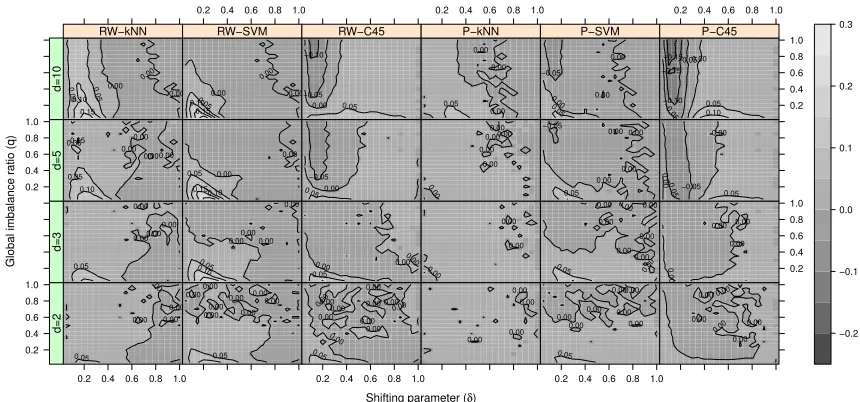
Figure 9 illustrates the difference between AUCs of CCCD and other classifiers (k-NN,
Shifting parameter (δ)
Global imbalance r
atio (q) 0.2 0.4 0.6 0.8 1.0
0.2 0.4 0.6 0.8 1.0
0.00 0.00 0.00 0.00 0.05 d=2 0.00 0.00
0.000.00 0.00
0.00 0.000.00
0.05
0.2 0.4 0.6 0.8 1.0
0.00
0.00 0.000.000.00
0.00 0.00 0.00 0.00 0.00 0.00 0.05 0.00 0.00 0.00 0.00
0.2 0.4 0.6 0.8 1.0
0.00 0.00 0.00 0.00 0.000.00 0.00 0.05 0.00 0.00 0.00 0.00 0.00 0.00 0.00 0.00 0.000.00 0.05 d=3 0.00 0.00 0.00 0.00 0.05
0.10 0.00 0.00
0.00 0.05 0.00 0.00 0.00 0.00 0.00 0.00 0.00 0.00 0.00 0.00 0.00 0.05 0.2 0.4 0.6 0.8 1.0 0.00 0.00 0.00 0.00 0.2 0.4 0.6 0.8 1.0 0.00 0.00 0.000.00 0.05 0.050.05 0.10 d=5 0.00 0.00 0.05 0.10 0.15 −0.05 0.00 0.05 0.00 0.00 0.00 0.00 0.00 0.00 −0.05 0.00 0.00 0.00 0.00 0.05 −0.05 −0.05 0.00 0.00 0.05 0.00 0.00 0.00 0.05 0.05 0.10 0.15 RW−kNN d=10
0.2 0.4 0.6 0.8 1.0
0.00 0.00 0.00 0.05 0.10 0.15 RW−SVM −0.10 −0.05 0.00 0.05 RW−C45
0.2 0.4 0.6 0.8 1.0
0.00 0.00 0.00 0.05 P−kNN −0.05 0.00 0.00 0.00 0.05 P−SVM
0.2 0.4 0.6 0.8 1.0
0.2 0.4 0.6 0.8 1.0 −0.15 −0.15 −0.10−0.05 −0.050.00 0.05 0.10 P−C45 −0.2 −0.1 0.0 0.1 0.2 0.3
Figure 9: Differences between the AUCs of CCCD and other classifiers. For example, the
panel titled with ”RW-kNN” presents AUC(RW-CCCD)-AUC(kNN). In this
two-class setting, two-classes are drawn fromFX =U(0,1)d and FY =U(δ,1 +δ)d with
d = 2,3,5,10. Each cell of the grey scale heat map corresponds to a single
combination of simulation parametersδ, q= 0.05,0.1,· · ·,0.95,1.00 withn= 400
andm=qn.
LNP, since it tends to perform better for imbalanced data sets, and we refer to C45-LNP as C4.5 for simplicity. Each cell of a single heat map is associated with a combination
of δ and q values. Lighter tone cells indicate that CCCD classifiers are better than the
other classifiers in terms of AUC, and vice versa for the darker tones. When the classes are imbalanced and moderately overlapping, RW-CCCD classifier has at least 0.05 more AUC than all other non-CCCD classifiers but P-CCCD classifier is only better than all others
provided that d = 10. If the classes are balanced or their supports are not considerably
overlapping, there seem to be no visible difference between CCCD and the other classifiers. Thus, the other classifiers suffer from the imbalance of the data while CCCD classifiers show robustness to the class imbalance. But more importantly, this difference is getting more
apparent with increasing dimensionality. Whendis high, fewer points of the minority class
fall in E although q(E) is fixed. Even though the classes are imbalanced, if the minority
class have substantially small size, the class imbalance problem becomes more detrimental (Japkowicz and Stephen, 2002). Under the conditions that the data set has substantial imbalance and overlapping, AUC of RW-CCCD classifier is followed, in order by, the AUC
of C4.5, SVM andk-NN classifiers.
Unlike the comparison of CCCD and SVM classifiers in Figures 5 and 8, SVM classifier
has less AUC than CCCD classifiers with low δ and low q values in Figure 9. In this
setting, n is fixed to 400 and the lowest value of m is 20. Compared to our experiments
more observations than the other, m << n). Akbani et al. (2004) conducted a detailed investigation and listed some reasons of SVM classifier being sensitive to highly imbalanced UCI data sets (Bache and Lichman, 2013). They did not, however, address the problem of overlapping class supports but offered a modification to SMOTE algorithm in order to
improve the robustness of SVM. On the other hand, especially ford= 5 and d= 10, SVM,
k-NN and C4.5 classifiers have more AUC than CCCD classifiers with increasing q and
decreasingδ. This may indicate that other weak classifiers are better than CCCD classifiers
for balanced classes.
The effects of class imbalance might also be observed when the class supports are well
separated. If the class supports are disjoint, that is s(FX)∩s(FY) = ∅, the AUC is fairly
high. However, it might still be affected by the global imbalance level, q. Therefore,
we simulate a data set with two classes where FX =U(0,1)d and FY =U(1 +δ,2 +δ)×
U(0,1)d−1. Figure 10 illustrates the results of this simulation study. Both class supports are
ddimensional unit boxes as in the previous simulation setting, however they are now disjoint
(separated along the first dimension). In addition, the parameter δ controls the smallest
distance between the class supports where δ = 0.05,0.10,· · · ,0.45,0.50. With increasing
δ, the points of classY move further away from the points of X. Figure 10 illustrates the
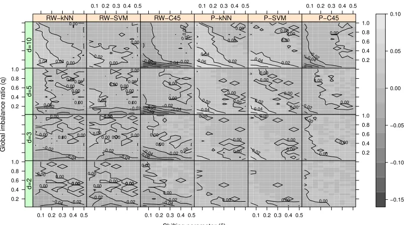
difference between AUCs of CCCD and other classifiers under this simulation setting. In Figure 10, unlike the performance of CCCD classifiers in Figure 9, P-CCCD classifiers have more AUC than RW-CCCD classifiers. When classes are imbalanced and supports are
close, P-CCCD classifiers outperform both SVM and k-NN classifiers for all dvalues, but
RW-CCCD classifiers have nearly 0.03 more AUC than these classifiers only in d = 10.
However, this is not the case with C4.5 classifier since none of the classifiers outperform C4.5; that is, C4.5 yields over 0.04 more AUC than CCCD classifiers. A well separated data set is more likely to be classified better with C4.5 tree classifier because a single separating line exists between the two class supports. Hence, C4.5 locates such a line and efficiently classifies points regardless of the distance between class supports as long as the distance is positive. On the other hand, the balls of P-CCCD classifiers establish appealing covers for the class supports because the supports do not overlap. P-CCCD classifiers establish covering balls, big enough to catch substantial amount of points from the same class. Similarly, RW-CCCD classifiers establish pure covers, and this is the result of the separation between class supports. However, P-CCCD classifiers achieve better classification performance than RW-CCCD classifiers. When the classes are well separated, the radii of a
ball in random walk, say from classX, is likely maxz∈Xnd(z, x) but in P-CCCD classifiers,
it is minz∈Ynd(z, x). In fact, the RW-CCCD classifiers are nearly equivalent to P-CCCD
classifiers. Thus, when τ > 0, P-CCCD classifiers are more likely to produce bigger balls
than RW-CCCD classifiers, and potentially avoid overfitting.
In Figure 10, RW-CCCD classifiers have slightly or considerably less AUC than other classifiers when data sets are imbalanced and the supports are slightly far away from each other. The random walk contaminates the class cover with some non-target class points to improve the classification performance. However, since the classes are well separated and one class has substantially fewer points than the other, random walks are likely to yield balls to cover some points from the support of the non-target class, resulting in a degradation in the performance of RW-CCCD classifiers. On the other hand, P-CCCD classifiers outperform
Shifting parameter (δ)
Global imbalance r
atio (q) 0.2 0.4 0.6 0.8 1.0
0.1 0.2 0.3 0.4 0.5
−0.04 −0.02 0.00 0.00 0.00 0.00 0.00 d=2 −0.02 −0.02 0.00 0.00 0.00 0.00 0.00
0.1 0.2 0.3 0.4 0.5
−0.04−0.02 0.00 0.00
0.00
0.1 0.2 0.3 0.4 0.5
0.00 0.00 −0.04 −0.02 0.00 0.00 0.00 0.00 d=3 −0.04 −0.02 0.00 0.00 0.00 0.00 0.00 0.00
−0.06−0.04 −0.02 0.00 0.00 0.00 0.00 0.00 0.00 0.00 0.00 0.00 0.02 0.2 0.4 0.6 0.8 1.0 0.00 0.00 0.00 0.2 0.4 0.6 0.8 1.0 −0.02 0.00 0.00 0.00 0.00 0.00 0.00 d=5 −0.02 0.00 0.00 0.00 0.00 0.00 0.00 0.00 −0.08−0.06 −0.04 −0.02 0.00 0.00 0.00 0.00 0.02 0.04 0.00 0.00 0.00 0.00 0.02 0.04 −0.02 0.00 0.00 0.00 0.00 0.02 0.04 RW−kNN d=10
0.1 0.2 0.3 0.4 0.5
0.00 0.00 0.02 RW−SVM −0.08 −0.06 −0.04−0.02 0.00 0.00 RW−C45
0.1 0.2 0.3 0.4 0.5
0.00 0.00 0.02 0.04 0.06 P−kNN 0.00 0.00 0.00 0.02 0.04 P−SVM
0.1 0.2 0.3 0.4 0.5
0.2 0.4 0.6 0.8 1.0 −0.04 −0.02 0.00 P−C45 −0.15 −0.10 −0.05 0.00 0.05 0.10
Figure 10: Differences between the AUCs of CCCD and other classifiers (see Figure 9 for
details). In this two-class setting, classes are drawn from FX = U(0,1)d and
FY =U(1+δ,2+δ)×U(0,1)d−1 whered= 2,3,5,10,δ = 0.05,0.1,· · ·,0.45,0.50
andq= 0.05,0.1,· · · ,0.95,1.00 withn= 400 andm=qn. AUCs of all classifiers
are over 88% since the class supports are well separated.
data, the better the performance of P-CCCDs than other classifiers. Although the classes do not overlap, the effect of class imbalance is still observed when the supports are close. When there is mild imbalance between classes, CCCD classifiers have either comparable or
less AUC. In addition, note that the performances of SVM andk-NN classifiers deteriorate
but P-CCCD classifiers preserve their AUC with increasing d. LetE ⊂Rd be some region
that contains points of both classes which are sufficiently close to the decision boundary.
With increasing d, fewer minority class points are in this region, and hence fewer members
of this class fall inE. As a result, the performance of both SVM andk-NN classifiers suffer
from local class imbalance with respect to E.
Finally, we investigate the effect of dimensionality when classes are balanced (i.e.,q= 1)
and their supports are overlapping. In this setting, FX =U(0,1)d and FY =U(δ,1 +δ)d.
Here, let q(E) ≈ q = 1, hence the classes are also locally balanced with respect to E as
well as being globally balanced. Also, δ controls the level of overlap between two classes.
However, we define δ in such a way that the overlapping ratio α ∈ [0,1] is fixed for all
dimensions. When α is 0, the supports are well separated, and whenα is 1, the supports
of classes are the same, i.e., s(FX) = s(FY). The closer α to 1, the more the supports
Dimensionality (d) Ov er lapping r atio ( α ) 0.2 0.4 0.6 0.8 1.0
5 10 15 20 −0.02
0.00
0.00 0.00
0.00 0.00 0.00
0.00 0.00 0.00 0.00 0.02 n=50 −0.02 −0.02 −0.02 −0.02 −0.02 0.00 0.00 0.00 0.00 0.00 0.00
5 10 15 20 0.00 0.00 0.00 0.00 0.00 0.00 0.00 0.00 0.00 0.00 0.00 0.02 −0.04 −0.02 0.00 0.00 0.00 0.00 0.00 0.00 0.00
5 10 15 20 −0.06 −0.04 −0.02 0.00 0.00 0.00 0.00 0.00 0.000.00 0.00 −0.02 0.00 0.00 0.00 0.00 0.00 0.000.00 0.00 0.02 −0.02 0.00 0.00 0.00
0.000.00 0.00
0.00 0.00 0.00 0.00 0.00 0.00 n=100 −0.02 0.00 0.00 0.00 0.00 −0.04 −0.02 0.00 0.00 0.00 0.00 0.00 0.00 0.00 0.00 0.00 0.00 0.00 −0.04 −0.02 0.00 0.000.00 0.00 0.00 0.00 −0.06 −0.04 −0.02 0.00
0.000.000.000.00 0.00
0.00 0.000.00
0.2 0.4 0.6 0.8 1.0 −0.08 −0.06 −0.04 −0.02 0.00 0.00 0.00 0.00 0.00 0.00 0.00 0.2 0.4 0.6 0.8 1.0 0.00 0.00 0.00 0.00 0.00 0.00 0.00 0.00 0.00 0.00 0.00 0.00 0.00 0.02 n=200 −0.02 −0.02 −0.02 0.00
0.000.000.00
0.00 0.00 −0.08 −0.08 −0.06 −0.04 −0.02 0.00 0.00 0.00 0.00
0.000.000.00
0.00 0.00 0.00 0.00 −0.04 −0.02 −0.02 0.00 0.00 0.00 0.00 0.000.00 0.00 −0.06−0.06 −0.04 −0.04 −0.02−0.02 0.00 0.00 0.00 0.00 0.00
0.00
0.00 0.00
−0.12 −0.10−0.08−0.06
−0.04 −0.02
0.00
0.00
0.00 0.000.00
0.00 0.00 0.00 0.000.00 0.000.00 0.00 0.000.000.00 0.00 0.00 0.00 RW−kNN n=500
5 10 15 20
−0.04 −0.02
−0.02 −0.02−0.02
−0.02 0.00 0.00 0.000.00 0.00 0.000.000.00 0.00 0.00 RW−SVM −0.12 −0.10 −0.08 −0.06 −0.04 −0.02 0.00 0.00 0.00 0.00 0.00 0.00 0.00 0.00 RW−C45
5 10 15 20
−0.04 −0.02 0.00 0.000.00 0.00 0.00 0.00 0.00 0.00 P−kNN −0.06 −0.06 −0.04−0.02 0.00
0.000.000.000.000.00
P−SVM
5 10 15 20
0.2 0.4 0.6 0.8 1.0 −0.18 −0.18 −0.18−0.16 −0.14−0.12 −0.10 −0.08 −0.06 −0.04
−0.020.00 0.00
0.00 0.00 0.000.00 0.00 P−C45 −0.20 −0.15 −0.10 −0.05 0.00 0.05
Figure 11: Differences between the AUCs of CCCD and other classifiers (see Figure 9 for
details). In this two-class setting, classes are drawn from FX = U(0,1)d and
FY =U(δ,1 +δ)d where n= 50,100,200,500, α = 0.05,0.1,· · · ,0.45,1.00 and
d= 2,3,4,· · · ,20.
dimensionalityd:
α = Vol(s(FX)∩s(FY))
Vol(s(FX)∪s(FY))
= (1−δ)
d
2−(1−δ)d ⇐⇒ δ= 1−
2α
1 +α
1/d
. (6)
Hence, we calculateδ for each (d, α) combination by the Equation (6). In Figure 11, each
cell of the grey scale heat map corresponds to a single combination of simulation parameters
α = 0.05,0.1,· · · ,0.95,1.00 and d = 2,3,4,· · · ,20. In Figure 11, the differences between
the AUCs of CCCD classifiers and other classifiers are up to 0.20. The k-NN and SVM
classifiers have comparable performance with CCCD classifiers, or outperform both CCCD
classifiers. However, C4.5 has more AUC with increasingd. Employing CCCD classifiers do
not considerably increase the classification performance over other classifiers when classes are balanced.
5.2 Empirical Comparison of CCCD-based and Strong Classifiers
In this section, we compare the CCCD-based classifiers with strong versions ofk-NN, SVM
and C4.5 classifiers on simulated data sets. Each classifier is modified in three different schemes, namely, resampling, ensemble and cost-sensitive schemes. We use SMOTE+ENN algorithm as the resampling scheme and EasyEnsemble algorithm as the ensembling scheme. As for the cost sensitive versions on weak classifier, we adjust the classifiers into
recogniz-ing class weights. For k-NN, we employ an algorithm giving more weight on neighboring
Method Description
SMOTE+ENN A combination of SMOTE (t = 2 and k = 5) and ENN (k = 3) (Batista et al., 2004).
EasyEnsemble A combination of undersampling (T= 4) and Adaboost (si= 10) for
i= 1,2,· · ·, T (Liu et al., 2009)
C5.0 The cost sensitive version of C4.5 (Kuhn and Johnson, 2013). CkNN A cost sensitive version ofk-NN (Barandela et al., 2003). CSVM A cost sensitive version of SVM (Chang and Lin, 2011).
Table 2: The description of classifiers employed in the article.
corresponding class; and for C4.5, we employ the C5.0. With three schemes and three weak classifiers, we get nine strong classifiers to study. We list and describe all these schemes in Table 2.
SMOTE+ENN algorithm, first, oversamples the entire training data set by generating artificial points in between a point and its neighbors. Specifically, for each point in the
data set, t points among k neighbors are selected, and until the data set is balanced,
new artificial points are generated in between these points and their selected neighbors. Later, ENN algorithm cleans the data set of noisy points by checking all points if the
majority of theirkneighbors are labeled as the class of the point. If not, the point is erased
from the data set. Simply, SMOTE+ENN is a hybrid of over and undersampling methods. EasyEnsemble algorithm is a hybrid of undersampling and ensemble methods. An ensemble
of weak classifiers is established by generating T many undersampled balanced data sets
from the training data set. Then, each data set is used to train individual Adaboost
classifiers with si many weak classifiers for i = 1,2, . . . , T. Hence, EasyEnsemble is an
ensemble ofPT
i=1si many weak classifiers.
We choose one of the simulation settings conducted in Section 5.1. Since CCCD classi-fiers are observed to be better than other classiclassi-fiers when both class imbalance and overlap-ping occurred, we only compare CCCD classifiers with strong classifiers on a single
simula-tion setting. Hence we choose the setting presented in Figure 9, i.e., we let FX =U(0,1)d
andFY =U(δ,1+δ)dfor buraδ, q= 0.05,0.10,· · ·,0.95,1.00,n= 400 andm=qn. We aim
to highlight the differences between the strong classifiers and CCCD classifiers for various combinations of overlapping and class imbalance ratios. The results on average AUCs of each strong classifier is given in Figure 12. In general, RW-CCCDs seem to perform better
than P-CCCDs. For d >2, P-CCCDs have nearly 0.10 less AUC than RW-CCCDs when
the classes are substantially overlapping and imbalanced, and it is observed that P-CCCDs are usually worse compared to the strong classifiers considered. However, the AUCs of RW-CCCD classifiers are either comparable or slightly less compared to others with the
most difference being seen in the case ofd= 10 when RW-CCCDs compared to EC4.5 and
C5.0, ensemble and cost sensitive versions of the C4.5 classifier, respectively. However, with
decreasingδandq, the RW-CCCDs have only 0.05 less AUC than others. Also, RW-CCCDs
Shifting parameter (δ)
Global imbalance r
atio (q) 0.2 0.4 0.6 0.8 1.0
0.2 0.4 0.6 0.8 1.0 0.00 0.00 0.00 0.00 0.00 0.000.00 0.00 0.00 0.00 0.00 0.00 d=2 0.000.00 0.000.00 0.00 0.00 0.00 0.00 0.00 0.00 0.00 0.00 0.00 0.00
0.2 0.4 0.6 0.8 1.0 0.000.00 0.00 0.00 0.00 0.00 0.00 0.00 0.00 0.00 0.00 0.00 0.00 0.00 0.00 0.00 0.00 0.00 0.00 0.00
0.2 0.4 0.6 0.8 1.0 0.00 0.00 0.000.00 0.00 0.00 0.00 0.00 0.00 0.00 0.00 0.00 0.00 0.00 0.00 0.00 0.00 0.00 0.00 0.00 0.00 0.00 0.00
0.2 0.4 0.6 0.8 1.0 0.00 0.00
0.000.00 0.000.00 0.000.00
0.00 0.00 0.00 0.00 0.00 0.00 0.00 0.00 0.00 0.00 0.00 0.00 0.00
0.2 0.4 0.6 0.8 1.0 0.00 0.00 0.00 0.00 0.00 0.00 0.00 0.00 −0.05 −0.050.00 0.00 d=3 −0.05 0.00 0.00 0.00 0.00 0.00 0.00 0.00 0.00 0.00 0.00 0.00 −0.05 0.00 0.00 0.00 0.00 0.00 0.00 0.00 −0.05 0.00 0.00 0.00 0.00 −0.05 0.00 0.000.000.000.00
0.00 0.00 0.00 0.000.00 0.00 −0.05 0.00 0.00 0.00 0.00 0.00 0.000.00 0.00 −0.05 0.00 −0.10 −0.05 0.00 0.000.000.00
0.00 0.00 0.00 0.000.00 0.00 0.00 0.2 0.4 0.6 0.8 1.0 −0.05 0.00 0.00 0.00 0.00 0.00 0.00 0.00 0.2 0.4 0.6 0.8 1.0 −0.10 −0.05 −0.05 0.00 0.00 0.00 0.00 d=5 −0.10 −0.05 −0.05 0.00 −0.10−0.05 0.00 0.000.00 0.00 0.00 0.00 0.00 0.00 −0.10 −0.05 −0.05 −0.05 0.00 0.00 0.00 0.000.00 −0.15 −0.10 −0.10 −0.05 0.00 −0.10−0.05 0.00 0.00 0.00 0.00 0.00 −0.10 −0.05 0.00 0.00 0.00 −0.10 −0.05 −0.05 0.00 0.05 −0.10 −0.05 0.00 0.00 −0.10 −0.05 −0.05 0.00 0.00 0.00 P−SkNN d=10
0.2 0.4 0.6 0.8 1.0
−0.10 −0.05 −0.05 0.00 0.00 P−SSVM −0.15 −0.10 −0.10 −0.05 −0.05 0.00 P−SC45
0.2 0.4 0.6 0.8 1.0
−0.10 −0.05 0.00 0.00 0.00 0.00 0.00 P−EkNN −0.05 −0.05 0.00 0.00 0.00 P−ESVM
0.2 0.4 0.6 0.8 1.0
−0.20 −0.20 −0.20 −0.15 −0.15 −0.10 −0.05 0.00 0.00 0.00 P−EC45 −0.15 −0.10 −0.05 −0.05 0.00 0.00 0.00 P−CkNN
0.2 0.4 0.6 0.8 1.0
−0.10 −0.05 −0.05 0.00 0.00 0.00 P−CSVM 0.2 0.4 0.6 0.8 1.0 −0.15 −0.10 −0.10−0.05 0.00 0.05 P−C50
−0.25 −0.20 −0.15 −0.10 −0.05 0.00 0.05 0.10 0.15
Shifting parameter (δ)
Global imbalance r
atio (q) 0.2 0.4 0.6 0.8 1.0
0.2 0.4 0.6 0.8 1.0 0.00 0.00 0.00 0.00 0.00 0.00 0.00 0.00 0.00 d=2 0.00 0.00 0.00 0.000.00 0.00 0.00 0.00 0.00 0.00 0.00
0.2 0.4 0.6 0.8 1.0 0.00 0.00 0.00 0.00 0.00 0.00 0.00 0.00 0.00 0.00 0.00 0.00 0.00 0.000.00 0.00 0.000.00 0.00 0.00 0.00
0.2 0.4 0.6 0.8 1.0 0.00 0.00 0.00 0.00 0.00 0.00 0.00 0.00 0.00 0.00 0.00 0.00 0.00 0.00 0.00 0.00
0.2 0.4 0.6 0.8 1.0
0.000.00 0.00 0.00 0.00 0.00 0.00 0.00 0.00 0.00 0.00 0.00 0.00 0.00 0.00 0.00 0.00 0.00 0.00 0.000.00 0.00 0.00 0.00 0.00 0.00 0.00 0.00 0.00 0.00 0.00
0.2 0.4 0.6 0.8 1.0 0.00 0.00 0.00 0.00 0.00 0.00 0.00 0.00 0.00 0.00 0.00 d=3 −0.05 0.00 0.00 0.00 0.00 0.00 0.00 0.00 0.00 0.000.00 0.00 0.00 −0.05 0.00 0.00 0.00 0.00 0.00 0.00 0.00 0.00 0.00 0.00 0.00 0.000.00 −0.05 0.00 0.000.00 0.00 0.00 0.000.00 0.00 0.00 0.00 0.000.00 0.00 0.00 −0.05 0.00 0.00 0.00 0.00 0.00 0.00 0.00 0.00 0.00 0.00 0.00 0.00 0.00 −0.05 0.00 0.00 0.00 0.00 0.000.00 0.00 0.00 0.000.00 0.00 0.00 0.00 0.00 0.00 0.00 0.2 0.4 0.6 0.8 1.0 −0.05 0.000.00 0.00 0.00 0.00 0.00 0.00 0.00 0.2 0.4 0.6 0.8 1.0 −0.05 0.00 0.00 0.00 d=5 −0.05 0.00 −0.05 0.00 0.00 0.00
0.00 0.000.00
−0.05 0.00 0.00 −0.05 0.00 0.000.00 −0.05 0.00 0.00 0.00 0.00 −0.05 0.00 0.00 0.00 −0.05 0.00 −0.05
0.00 0.000.00
−0.05 0.00 0.00 0.00 RW−SkNN d=10
0.2 0.4 0.6 0.8 1.0
−0.05 0.00 0.00 RW−SSVM −0.05 −0.05 −0.05 0.00 RW−SC45
0.2 0.4 0.6 0.8 1.0
−0.05 0.00 0.00 0.00 0.05 0.05 0.05 0.05 RW−EkNN 0.00 0.00 0.00 0.05 RW−ESVM
0.2 0.4 0.6 0.8 1.0
−0.15 −0.10 −0.05 0.00 0.00 RW−EC45 −0.05 0.00 0.00 RW−CkNN
0.2 0.4 0.6 0.8 1.0
−0.05 0.000.00 0.00 0.00 RW−CSVM 0.2 0.4 0.6 0.8 1.0
−0.10−0.10−0.050.00
0.05 RW−C50
−0.20 −0.15 −0.10 −0.05 0.00 0.05 0.10 0.15
Figure 12: Differences between the AUCs of CCCD and other classifiers (see Figure 9 for de-tails). P-CCCD in (top) and RW-CCCD in (bottom). Here, resampling scheme strong classifiers are coded with “S”, ensemble schemes with “E”, and cost sensi-tive schemes with “C”. For example, “SkNN” refers to the resampling schemed
k-NN classifier. In this two-class setting, classes are drawn fromFX =U(0,1)d
and FY =U(δ,1 +δ)d where d= 2,3,5,10, q, δ = 0.05,0.1,· · ·,0.95,1.00 with