Integrative Analysis using Coupled Latent Variable Models
for Individualizing Prognoses
Peter Schulam [email protected]
Suchi Saria [email protected]
Department of Computer Science Johns Hopkins University Baltimore, MD 21218, USA
Editor:Benjamin M. Marlin and C. David Page
Abstract
Complex chronic diseases (e.g., autism, lupus, and Parkinson’s) are remarkably hetero-geneous across individuals. This heterogeneity makes treatment difficult for caregivers because they cannot accurately predict the way in which the disease will progress in order to guide treatment decisions. Therefore, tools that help to predict the trajectory of these complex chronic diseases can help to improve the quality of health care. To build such tools, we can leverage clinical markers that are collected at baseline when a patient first presents and longitudinally over time during follow-up visits. Because complex chronic diseases are typically systemic, the longitudinal markers often track disease progression in multiple organ systems. In this paper, our goal is to predict a function of time that models the future trajectory of a single target clinical marker tracking a disease process of interest. We want to make these predictions using the histories of many related clinical markers as input. Our proposed solution tackles several key challenges. First, we can easily handle irregularly and sparsely sampled markers, which are standard in clinical data. Second, the number of parameters and the computational complexity of learning our model grows linearly in the number of marker types included in the model. This makes our approach applicable to diseases where many different markers are recorded over time. Finally, our model accounts for latent factors influencing disease expression, whereas standard regres-sion models rely on observed features alone to explain variability. Moreover, our approach can be applied dynamically in continous-time and updates its predictions as soon as any new data is available. We apply our approach to the problem of predicting lung disease trajectories in scleroderma, a complex autoimmune disease. We show that our model im-proves over state-of-the-art baselines in predictive accuracy and we provide a qualitative analysis of our model’s output. Finally, the variability of disease presentation in sclero-derma makes clinical trial recruitment challenging. We show that a prognostic tool that integrates multiple types of routinely collected longitudinal data can be used to identify individuals at greatest risk of rapid progression and to target trial recruitment.
Keywords: gaussian processes, conditional random fields, prediction of functional targets, latent variable models, disease trajectories, precision medicine
1. Introduction
because caregivers cannot easily predict an individual’s future trajectory to guide therapy decisions. For example, in scleroderma, an autoimmune disorder, lung disease is a common cause of morbidity and mortality (Varga et al., 2012), but there are no known biomarkers or precise algorithms for stratifying individuals into groups based on similar lung disease course. A tool that can provide accurate forecasts of disease progression can help clinicians to tailor treatments to each patient based on their most likely course.
To monitor disease progression, clinicians collect many clinical markers both at baseline when an individual first visits the clinic and longitudinally during routine follow-up visits. Many CCDs are systemic, and so the markers are designed to monitor the disease’s impact across many organ systems. In scleroderma, individuals may be affected across six organ system—the lungs, heart, skin, gastrointestinal tract, kidneys, and vasculature—to varying extents (Varga et al., 2012). Example clinical markers include PFVC (percent of predicted forced vital capacity), which is used to measure lung damage severity; TSS (total skin score), which is used to measure skin disease activity; and, PDLCO (percent of carbon monoxide diffused by the lung), used to measure vasculature health.
Our goal is to predict a function of time that models the future trajectory of a single target clinical marker tracking a disease process of interest. We want to make these pre-dictions by leveraging baseline information and additional time-dependent clinical markers (henceforth referred to as auxiliary markers) as they are collected. This is the focal challenge of personalized medicine: integrative analysis of heterogeneous data from an individual’s medical history to improve care (Collins and Varmus, 2015). So far, efforts in integrative analysis have focused on combining inferences from molecular data modalities (Rosenbloom et al., 2013). Our focus in this paper is on leveraging routinely recorded information from the electronic health record—both static and time-dependent—to make precise estimates of an individual’s disease course.
A key challenge in this setting is that these data are collected during routine clinical visits and therefore they are sparse and irregularly sampled. Predicting an individual’s future disease is commonly framed as a regression problem where the target clinical marker at a specific time in the future is modeled as a function of observed input features alone. These features are computed by generating summaries from the observed data (e.g., the last PFVC value or the trend in the PFVC over the last six months). However, training conditional models is less straightforward from data where varying numbers of repeated measurements are sampled per patient and across different markers. In this setting, others have focused on dynamical prediction (e.g., Rizopoulos and Ghosh 2011; Proust-Lima et al. 2014) by fitting parametric models to the longitudinal data and using the resulting model parameters as features for prediction. But existing formulations do not scale to high-dimensional problems with many auxiliary markers.
repeated measurements of clinical marker data in the electronic health record. Schulam and Saria (2015) extend these ideas and introduce a transfer learning framework for predicting individual-specific disease trajectories that accounts for subtypes and other latent factors causing heterogeneity in disease expression. These works, however, focus on modeling single marker trajectories. We build on Schulam and Saria (2015) in this paper.
1.1 Contributions
In this paper, we describe a scalable framework for predicting a target marker trajectory (i.e. a continuous-time function) that allows us to use multiple longitudinal clinical marker histories as inputs. Our approach makes it easy to handle irregular sampling patterns across markers. Because we use a discriminative training criterion that conditions on marker his-tories instead of jointly modeling them, the framework is not as sensitive to misspecified dependencies across marker types. Moreover, the number of parameters and computational complexity scales linearly with the number of markers, which makes it possible to apply our approach in high-dimensional settings where many different marker types are available. Finally, our approach aligns with the dynamical nature of clinical medicine; it can be used to make predictions using continuously growing marker histories. We apply our approach to the problem of predicting lung disease trajectories in scleroderma, a complex autoimmune disease. We show that our model improves over state-of-the-art baselines in predictive accu-racy and we provide a qualitative analysis of our model’s output. Moreover, we demonstrate the clinical utility of our model by measuring performance on early detection of individuals who develop aggressive lung disease.
2. Related Work
Most predictive models used in medicine are cross-sectional—they use features from data measured up until the current time to predict a clinical marker or outcome at a fixed point in the future. As an example, consider the mortality prediction model by Lee et al. (2003), where logistic regression is used to integrate features into a prediction about the probability of death within 30 days for a given patient. To predict the outcome at multiple time points, it is common to fit separate models (e.g., Wang et al. 2012; Zhou et al. 2011). These models are trained to use features extracted from a fixed-size window, rather than a dynamically growing history. Moreover, they tackle heterogeneity in a limited way—any differences across individuals must be explained by observed features alone.
A common approach to dynamical prediction of trajectories is to use Markov models such as order-p autoregressive models (AR-p), HMMs, state space models, and dynamic Bayesian networks (e.g. Hassan and Nath 2005; Quinn et al. 2009; Murphy 2002). While such models naturally make dynamic predictions using the full history by forward-filtering, they typically assume discrete, regularly-spaced observation times.
has too few observations, which is common in clinical data. James and Sugar (2003) address this issue by modeling the parameters of individual trajectories as random variables with a low-rank parameterization of the mean and covariance. This work is closely related to ours, and the idea of sharing statistical strength across trajectories through a structured prior over individual-specific parameters is used broadly throughout trajectory analysis to account for sparsity. Gaussian processes (GPs) are also commonly used in FDA; they offer flexible nonparametric models of trajectories but can also help to counteract sparsity by sharing kernel hyperparameters across individuals—see Roberts et al. (2013) for a recent review of GPs applied to time series data. Recent work by Liu and Hauskrecht (2014) combines the advantages of Markov models (e.g. AR processes and state space models) and Gaussian processes to make predictions of clinical laboratory test results. To account for variability in collections of functions, a number of authors have proposed variants of GPs that account for variability in the mean function (e.g. L´azaro-Gredilla et al. 2012; Shi et al. 2012) and the covariance function (e.g. Shi et al. 2005). Another related line of work in the FDA literature is function-to-function regression (e.g., Oliva et al. 2015). In most approaches to function-to-function regression (FFR) the input and output are defined on fixed domains. In contrast, our problem requires updated predictions as the clinical history continues to grow; both the input and output domains are therefore constantly changing.
Most related to our work is that by Rizopoulos (2011), where the focus is on making
dynamical predictions about a time-to-event outcome (e.g. time until death) using all
previously observed values of a longitudinally recorded marker. As more data is collected, they dynamically update posterior distributions over individual-specific longitudinal model parameters (as is done in FDA), which serve as time-varying features for the time-to-event prediction. Proust-Lima et al. (2014) tackles the same task but uses a mixture of trajectories to model longitudinal data. As more observations are collected, the posterior over a set of classes is updated, each of which has a distinct set of time-to-event model parameters. These are both state-of-the-art models for the task of dynamical disease trajectory prediction; we will revisit them in our experimental section where we use the approaches as baselines. To scale these models to multivariate time series, however, requires careful specification of the joint model across different markers, which can be challenging in high-dimensional settings (e.g., D¨urichen et al. 2015) and may be difficult to scale. For example, Rizopoulos and Ghosh (2011) use a random effects model with a full covariance matrix to describe dependencies across markers, which scales quadratically in the number of marker types (as opposed to linearly as is the case for C-LTM). Because C-LTM is discriminatively trained (we optimize the likelihood of future target trajectories given target and auxiliary marker histories), it is less sensitive to misspecification of the dependencies across markers.
3. Coupled Latent Trajectory Model
(a) (b) (c) 376 1013 ● ● ● ● ● ●●● ● ● ● ● ● ●●● ● ● ● ● ● ●● ● ● ● ● ● ●●●●● ●●● ● ● ● ● ● ●● ● ● ● ● ● ● ●●● ● ● ● ● ● ●● ● ● ● ● ● ●●●●● ●●● ● ● ● ● ● ●●● ● ● ● ● ● ●●● ● ● ● ● ● ●● ● ● ● ● ●● ●●●● ●●● ● ● ● ● ●● ●●●●● ● ●● ● ● ● ●● ● ● ● ● ● ● ● ● ● ● ●●●● ●●● ● ●● ● ● ● ● ● ● ● ● ● ● ● ● ● ● ● ●●●● ●●● ● ●● ● ● ● ●● ● ● ● ● ● ● 60 70 80 90 60 70 80 90 60 70 80 90 Subtype Subtype+Long Subtype+Long+Shor t
0 5 10 15 0 5 10 15
Years Since First Symptom
pFVC Level Subtype Subtype+Long Subtype+Long+Short 771 1159 ● ● ●● ● ● ● ● ●● ● ● ● ● ● ●● ● ● ● ● ●● ● ● ● ● ● ●● ● ● ● ● ●● ● ● ● ● ● ● ● ● ● ●●● ● ● ●●●● ● ● ● ● ● ● ●● ●●● ● ● ● ● ● ● ● ●● ● ● ●●●● ●● ● ● ● ● ●● ●●● ● ● ● ● ● ● ● ●● ● ● ●●●● ●● ● ● ● ● ●● ●●● 50 60 70 80 50 60 70 80 50 60 70 80 Subtype Subtype+Long Subtype+Long+Shor t
0 5 10 15 0 5 10 15 Years Since First Symptom
pFVC Level Subtype Subtype+Long Subtype+Long+Short PFVC (d)
Years Since First Symptom
PFVC
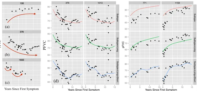
Figure 1: Plots (a-c) show example marker trajectories. Plot (d) shows four individuals with ad-justments to a population and subpopulation fit (row 1). Row 2 makes an individual-specific long-term adjustment. Row 3 makes individual-individual-specific short-term adjustments. To simplify, we only show mean functions; posterior uncertainty intervals are omitted.
Input: Baseline predictors
Target marker trajectories Auxiliary marker trajectories
Stage 1: Fit Latent Trajectory Models (Model in Sec. 3.2, learning in Sec. 3.5)
Fit target marker LTM to define factor For
Fit auxiliary marker LTM to define factor
Stage 2: Fit Coupling Model (Model in Sec. 3.3 & 3.4, learning in Sec. 3.5) ~
x1:N
~
y1:N
Initialize singleton factor weights for
Fit CRF parameters by maximizing Initialize pairwise factor weights for (·,·)
, , and for
For each regularization penalty
Refit CRF using full training set with best Fit CRF on training data:
Evaluate penalty on development data
c2{1, . . . , C}
`c,i,t(·)
`i,t(·)
`i,t(·) `c,i,t(·) c2{1, . . . , C}
(·)
~ y1:C,1:N
J( , 1:C,✓,✓1:C,⌘1:C),
M
X
i=1
X
t2T
logp(~yi,>t|~yi,t,~y1:C,i,t,~xi)
(k , 1:Ck1+k✓,✓1:Ck1+k⌘1:Ck1)
Figure 2: Two-stage procedure for fitting the Coupled Latent Trajectory Model (C-LTM).
distribution over the PFVC values (blue and green shaded regions) are conditioned upon baseline markers (e.g. gender and race), the observed PFVC values (black points), and
auxiliary marker histories (e.g. TSS). We learn our model from a database of clinical
model will estimate the following conditional distribution (notation is described in the subsequent paragraph):
D(i, t),p(yi(·)|y~i,≤t, ~y1:C,i,≤t, ~xi). (1)
Notation. For an individuali, we denote each target marker observation usingyij and its
measurement time usingtij wherej∈ {1, . . . , Ni}. We use~yi ∈RNi and~ti∈RNi to denote all of individuali’s marker values and measurement times respectively. We assume that the target marker observations are noisy observations of a latent continuous-time function (the trajectory), which we denote usingyi(·). Each individual has baseline (static) information collected into a vector, which we denote using~xi. We useCto denote the number of auxiliary
marker types,Ncito denote the number of observations of thecth type, and useycij andtcij
to denote individuali’sjthmeasurement of marker typec. We use~yci∈RNci and~tci∈RNci to denote the vector containing all of individuali’scthmarker values and times respectively. We will also frequently need to refer to the vector of marker values observed up until a time
t, which we denote using~yi,≤t(~yci,≤tfor auxiliary markers). Similarly, for markers observed
after a time t, we use ~yi,>t (~yci,>t for auxiliary markers). The term ~y1:C,i,≤t refers to all
auxiliary markers measured on individual iup until timet.
At a high-level, we will model Eq. 1 by first assuming that each clinical marker trajectory (both target and auxiliary) can be d-separated (rendered conditionally independent) of all other marker types given a marker type-specific latent variable. We denote these latent variables using zi for the target marker and zci for auxiliary marker c, and will describe
them further later in this section. Under this assumption, we can write Eq. 1 as
D(i, t) =X
zi
p(y(·)|zi, ~yi,≤t, ~xi)p(zi |~yi,≤t, ~y1:C,i,≤t, ~xi)
∝X
zi
p(y(·)|zi, ~yi,≤t, ~xi)p(~yi,≤t|zi, ~xi)p(zi |~y1:C,i,≤t, ~xi)
∝X
zi
p(y(·)|zi, ~yi,≤t, ~xi)
| {z }
LTM predictive, Section 3.2.2,
Eq. 24
p(~yi,≤t|zi, ~xi)
| {z }
LTM likelihood, Section 3.2.1,
Eq. 16
X
z1:C,i
p(zi, z1:C,i|~xi)
| {z }
Coupling Model, Section 3.3,
Eq. 25
C Y
c=1
p(~yci,≤t|zci, ~xi).
| {z }
LTM likelihood, Section 3.2.1,
Eq. 16
(2)
3.1 Preliminaries
The Latent Trajectory Model (LTM) uses B-splines to model longitudinal trajectories, and our coupling model uses a conditional random field (CRF). We briefly introduce these two concepts, and point to resources where the interested reader can find additional details.
3.1.1 B-Splines
A common approach to fitting nonlinear functions of time while maintaining a linear de-pendence on model parameters is to use a basis expansion. Such an expansion defines some non-linear functionf(t) as a linear combination of other functions φ1(t), . . . , φd(t):
y=f(t|β) =
d X
i=1
βdφd(t) = Φ>(t)β,~ (3)
whereφ1, . . . , φdact as bases in some vector space of nonlinear functions and Φ(t)∈Rdis the vector containing the values of thepbasis functions evaluated at timet. The benefit of this formulation is that the function f is linear in the model parametersβ, making it relatively easy to fit complex models. B-splines are a particular family of basis functions that we can use to parameterize nonlinear functions. Others include polynomial bases and radial basis functions. However, there are two advantages to using B-splines. First, each basis function is non-zero only over a compact interval of the real line, which improves statistical stability and also allows for computational speed ups that take advantage of sparse basis matrices (Gelman et al., 2014). This is in contrast to polynomials, where each basis takes non-zero values globally. The second advantage is that the family of functions parameterized by B-splines are not infinitely differentiable (in contrast to radial basis functions) and therefore not smooth (Gelman et al., 2014). This bias is often helpful in modeling functions from the real-world that arise from non-smooth processes. Because B-splines are linear in their parameters, we can use the well-developed machinery of linear regression for learning. See Ch. 20 in Gelman et al. (2014) or Ch. 5 in Friedman et al. (2001) for further details.
Penalized B-splines. In practice, the parameters of a B-spline model are fit using a penalized least squares criterion. The penalty is typically introduced in order to control the smoothness of the fit. For data ~y measured at times~twith corresponding basis matrix Φ(~t) = [Φ(t1), . . . ,Φ(tn)]>, we minimize the following objective:
J(β~) =k~y−Φ(~t)β~k22+ρ~β>Ωβ,~ (4) where Ω is a first-order differences matrix as described by Eilers and Marx (1996). The penalized objective is still quadratic in β~ and so can be easily minimized.
3.1.2 Conditional Random Fields
output y, input x and parametersθ, the conditional probability is defined to be:
p(y|x, θ) = 1
Z(x, θ) Y
c
ψc(yc|x, θ), Z(x, θ), X
y0 Y
c
ψc(yc0 |x, θ), (5)
where ψc(yc | x, θ) is a non-negative factor that can be interpreted as scoring the
con-figuration of the subset of variables yc given the observations x and parameters θ. The
termZ(x, θ) is called thepartition function and ensures that the distribution is normalized. When we can write
logψc(yc|x, θ) =θc>fc(yc, x) ⇐⇒ ψc(yc|x, θ) = exp n
θc>fc(yc, x) o
, (6)
where fc extracts some vector of features from the observations x and the target yc, then
we say that the CRF is a log-linear model. Log-linear models have a number of desirable properties, the most relevant to this work being the ease with which we can differentiate the log-likelihood with respect to model parameters. To compute the derivative with respect toθc(the parameters corresponding to the cth factor) we have:
∂logp(y|x, θ)
∂θc
=fc(yc, x)−
∂logZ(x, θ)
∂θc
. (7)
To compute the partial derivative in the second term on the RHS, first note that
∂Z(x, θ)
∂θc
=X
y0
Y
d6=c
ψd(y0d|x, θd
∂ψc(yc0 |x, θc)
∂θc
(8)
=X
y0
Y
d6=c
ψd(y0d|x, θd
ψc(y0c|x, θd)fc(yc0, x). (9)
This implies that the partial derivative of logZ(x, θ) is simply:
∂logZ(x, θ)
∂θc
= 1
Z(x, θ)
∂Z(x, θ)
∂θc
=Ey[fc(yc, x)|x] (10)
This means that the gradient of the log-likelihood with respect to a set of parameters θc
is the difference between the observed features fc(y, x) and their expectation under the
current set of parametersθ. To learn the weights, we can apply gradient-based algorithms to optimize the likelihood of a set of observed training input-output pairs. In addition, a regularizer is often added to the objective to discourage complexity or induce sparsity. We will use these ideas in the derivation of our learning algorithm. See Ch. 19 in Murphy (2012) for further details.
3.2 Latent Trajectory Model
Subtype marginal probability
z
ifi
M
↵
yij tij
N
i~
g
G
~bi
⌃b ~ ⇢i
Population model features Population model coefficients
Long-term level features-to-coefficient map Subtype B-spline coefficients
Subtype indicator 2{1, . . . , G}
Long-term coefficients covariance matrix2Rd`⇥d` Long-term level coefficients2Rd`
Short-term level GP hyper-parameters
Short-term level effects2RR
2Rdz
2Rqp
2Rdp
2Rdp⇥qp
⇤
⇡
g2R
~
x
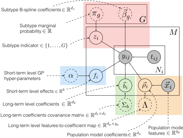
iFigure 3: The LTM graphical model. Levels in the hierarchy are color-coded. Model parameters are enclosed in dashed circles. Observed variables are shaded.
noisy observations of the underlying disease activity trajectory, which is a function of both individual-specific parameters and parameters that are shared across other individuals in the population. Moreover, the LTM uses individual-specific latent factors to explain dif-ferences in trajectories across the population that are not explained by observed features alone. The LTM graphical model is shown in Figure 3. We review the LTM below using the same notation defined at the beginning of this section. In addition, we use Φ(tij) to denote a
column-vector containing a basis expansion of the timetij and Φ ~ti
= [Φ(ti1), . . . ,Φ(tiNi)]
> to denote the matrix containing the basis expansion of points in~ti in each of its rows.
The LTM models thejth marker value for individualias a normally distributed random variable with a mean assumed to be the sum of four terms: a population component, a subpopulation component, an individual long-term component, and an individual short-term component.
yij|zi,~bi, fi∼ N
Φp(tij)
>Λ~x i
| {z }
(A) population
+ Φz(tij)>β~zi
| {z }
(B) subpopulation
+ Φ`(tij)>~bi
| {z }
(C) ind. long-term
+ fi(tij) | {z }
(D) ind. short-term , σ2
.
long-term component shares strength across all observations belonging to the same individ-ual. Finally, the individual short-term component shares information across observations belonging to the same individual that are measured at similar times. Predicting an individ-ual’s trajectory involves estimating her subtype and individual-specific parameters as new clinical data becomes available. We briefly review each of the components here for ease of presentation, but refer the interested reader to Schulam and Saria (2015) for further details.
Population level. The population model predicts aspects of an individual’s disease ac-tivity trajectory using observed baseline characteristics (e.g. gender and race), which are represented using the feature vector ~xi. This sub-model is shown within the orange box
in Figure 3. The predicted value of the jth marker of individuali measured at timetij is
shown in Eq. 11 (A), where Φp(t)∈ Rdp is a basis expansion of the observation time and Λ∈Rdp×qpis a matrix used as a linear map from an individual’s covariates~x
i to coefficients
ρi ∈Rdp. At this level, individuals with similar covariates will have similar coefficients.
Subpopulation level. LTM models an individual’s subtype using a discrete-valued latent variable zi ∈ {1, . . . , G}, where G is the number of subtypes. zi is a multinomially
dis-tributed random variable with parametersπ1:G,[π1, . . . , πG] whereπg ≥0 andPgπg = 1.
Each subtype has a unique disease activity trajectory represented using B-splines, where the number and location of the knots and the degree of the polynomial pieces are fixed prior to learning. These hyper-parameters determine a basis expansion Φz(t) ∈Rdz mapping a timet to the B-spline basis function values at that time. Trajectories for each subtype are parameterized by a vector of coefficients β~g ∈ Rdz for g ∈ {1, . . . , G}, which are learned offline. Under subtype zi, the predicted value of marker yij measured at time tij is shown
in Eq. 11 (B). This component explains differences such as those observed between the trajectories in Figures 1a and 1b.
Individual long-term level. The individual long-term component is parameterized using a linear model with basis expansion Φ`(t) ∈ Rd` and individual-specific coefficients ~b
i ∈
Rd`. This level models deviations from the population and subpopulation models using parameters that are learned dynamically as the individual’s clinical history grows. An individual’s coefficients are modeled as latent variables with marginal distribution ~bi ∼
N(~0,Σb). For individuali, the predicted value of markeryij measured at timetij is shown
in Eq. 11 (C). This component can explain, for example, differences in overall health due to an unobserved characteristic such as chronic smoking, which may cause atypically lower lung function than what is predicted by the population and subpopulation components. Such an adjustment is illustrated across the first and second rows of Figure 1d.
Individual short-term level. Finally, the individual short-term component fi captures
transient trends in an individual’s marker sequence that do not generalize outside of a small time window. For example, an infection may cause an individual’s lung function to temporarily appear more restricted than it actually is, which may cause short-term trends like those shown in Figure 1c and the third row of Figure 1d. We treat fi as a
function-valued latent variable and model it using a Gaussian process with zero-function-valued mean function and Ornstein-Uhlenbeck (OU) covariance function
KOU(t1, t2) =a2exp
−`−1|t1−t2| . (12)
to occur. The OU kernel is ideal for modeling such deviations as it is both mean-reverting and draws from the corresponding stochastic process are only first-order continuous, which eliminates long-range dependencies between deviations (Rasmussen and Williams, 2006). Applications in other domains may require different kernel structures motivated by proper-ties of transient deviations in the trajectories.
Accounting for treatments. Several interventions are common in scleroderma, but none have been proven to significantly alter the long-term course of the disease. For example, steroids are commonly administered, but there have been no randomized controlled trials confirming its effects on patients with scleroderma-related lung disease—see, for example,
Ch. 35 in Varga et al. (2012). Immunosuppressants are also commonly used to treat
scleroderma-related lung disease, but the proven effects are modest and have only been demonstrated over the course of one year (Tashkin et al., 2006). We assume that these types of transient interventions are well-modeled by the individual-specific short-term component, and so we do not explicitly model the treatment effects of steroids or immunosuppressants in our data. Others have developed methods for estimating treatment effects from observa-tional time series (e.g., Chib and Hamilton 2002; Kleinberg and Hripcsak 2011; Brodersen et al. 2015). More recently, see Xu et al. (2016) for an application using functional data. Treatment effects can be incorporated within the trajectory likelihood in diseases where treatments are suspected to alter long term trajectory. We leave this more general case as a direction for future work.
Missing data mechanism. The LTM assumes observations of the trajectory are missing at random (MAR). This implies that we can use maximum likelihood estimation without needing to incorporate additional information about the sampling model; see Appendix B. When the data are missing not at random, assumptions about the missing data mechanism should be explicated and incorporated within the individual marker models.
In summary, the latent, individual-specific factors in the model (zi,~bi, and fi from
Eq. 11B, 11C, and 11D respectively) each contribute to describe the observed trajectory at different granularities. These are all treated as random variables and marginalized out during learning to avoid overfitting. When making predictions, we can use an individual’s observed data to compute posterior distributions over these latent factors, which allows us to tailor predictions.
3.2.1 LTM Likelihood
Given parameters Θ = {Λ, π1:G, ~β1:G,Σb, a, `, σ2}, we can compute the observed-data
like-lihood of a given clinical marker trajectory by marginalizing zi,~bi and fi out of the joint
distribution defined by our model:
p(~yi |~xi,Θ)
=
G X
zi=1
p(zi|Θ)
| {z }
Multinomial prior
Z
Rd`
p~bi|Θ
| {z }
Normal prior
Z
RNi
p(fi |Θ)
| {z }
GP prior
p~yi |zi,~bi, fi, ~xi, ~ti,Θ
| {z }
Eq. 11
dfid~bi (13)
=
G X
zi=1
πziN
~
yi |Φp ~ti
Λ~xi+ Φz ~ti
~
βzi, K ~ti, ~ti
Moving from Eq. 13 to Eq. 14, we evaluate the innermost integral using the fact that the GP prior overfi is conjugate to Eq. 11 yielding a new multivariate normal (Rasmussen and
Williams, 2006). To evaluate the next integral in Eq. 13, we again have that the normal prior over~bi is conjugate to the multivariate normal obtained by marginalizing over fi,
which gives us the multivariate normal shown in Eq. 14 where the covariance function is defined as
K(t1, t2) = Φ`(t1)>ΣbΦ`(t2) +KOU(t1, t2) +σ2I(t1=t2). (15) We see that the observed-data likelihood for individual i is defined by a mixture of multi-variate normals where each subtype is associated with a class in the mixture. The mixing probabilities are defined by the multinomial over subtypes. The mean of the multivariate normal is defined by the population and subpopulation models, and the covariance is de-fined by the individual long-term and short-term components of the model. To obtain the LTM likelihood needed in Eq. 2, we will condition Eq. 14 on subtype zi. This gives us the
following expression:
p(~yi |zi, ~xi),N
~yi|Φp ~ti
Λ~xi+ Φz ~ti
~
βzi, K ~ti, ~ti
. (16)
3.2.2 LTM Predictive
As presented, the LTM can be easily applied to the task of disease activity trajectory predic-tion. Note that the LTM provides a posterior distribution over the trajectory using baseline markers and measurements of the target marker (e.g. PFVC) as they are recorded. It does not incorporate information from other time-varying markers such as TSS and PDLCO. Suppose we have estimates of the model parameters Θ = {Λ, π1:G, ~β1:G,Σb, a, `, σ2}, then
we can predict an individual’s future course by computing the posterior predictive distri-bution p(~yi,>t |~yi,≤t, ~xi), where ~yi,>t denotes marker values after time t and ~yi,≤t denotes
marker values observed prior to time t. To compute the expected marker value at timet∗i, we evaluate the following expression:
ˆ
y(t∗i) =
G X
zi=1
Z
Rd`
Z
RNi
E
h
y∗i |zi,~bi, fi i
| {z }
prediction given latent vars. p
zi,~bi, fi |~yi,≤t, xip,Θ
| {z }
posterior over latent vars.
dfid~bi (17)
=E∗z
i,~bi,fi
h Φp(t∗i)
>
Λ~xi+ Φz(t∗i) >~
βzi+ Φ`(t
∗ i)
>~b
i+fi(t∗i) i
(18)
= Φp(t∗i) >
Λ~xi
| {z }
pop. prediction
+ Φz(t∗i) >
~ β∗
i
z }| {
E∗zi
h
~ βzi
i
| {z }
subpop. prediction
+ Φ`(t∗i) >
~b∗
i
z }| {
E~b∗
i
h
~bi i
| {z }
ind. long prediction
+
fi∗(t∗i)
z }| {
E∗fi[fi(t
∗ i)]
| {z }
ind. short prediction
, (19)
where E∗ denotes an expectation conditioned on ~yi,≤t, xi,Θ. We see that the prediction
which is easily done given that the observed-data likelihood has a mixture of multivariate normals density (Eq. 14). The posterior probability of subtypegfor individualiis therefore
πig∗ ∝πg N
~
yi |Φp ~ti
Λ~xi+ Φz ~ti
~
βg, K ~ti, ~ti
. (20)
To compute the subpopulation prediction in Eq. 19 above, we simply compute the expected value of the B-spline coefficients under the posterior in Eq. 20:
~ βi∗,
PG
zi=1π
∗ izi
~ βzi
. (21)
The expectation required for the individual long-term prediction is:
~b∗ i ,
h
Σ−b1+ Φ`(~ti)>Kf−1Φ`(~ti)
i−1h
Φ`(~ti)>Kf−1
~
yi−Φ>p(~ti)Λ~xi−Φ>z(~ti)β~∗i i
. (22)
Finally, the expectation required for the individual short-term prediction is:
f∗(t∗i),KOU(t∗i, ~ti)
KOU(~ti, ~ti) +σ2I
−1
~ri (23)
where~ri=
~
yi−Φ>p(~ti)Λ~xi−Φ>z(~ti)β~∗i −Φ > ` (~ti)~b∗i
For brevity, we omit the derivation of these expectations here, but point the interested reader to Schulam and Saria (2015) and its supplementary material for the steps taken to arrive at these expressions. To obtain the LTM predictive needed in Eq. 2, we condition Eq 19 on subtypezi. This gives us the following expression:
p(y(·)|zi, ~yi,≤t, ~xi),Φp(·)>Λ~xi+ Φz(·)>β~zi+ Φ`(·)
> E~b∗
i
h
~bi i
+E∗fi[fi(·)]. (24)
3.3 Coupling Model
The Coupled Latent Trajectory Model (C-LTM) seeks to learn and capture correlations across trajectories of different marker types. In scleroderma, for example, an individual with worse lung trajectories (e.g. the rapidly declining lung trajectory subtype) is more likely to have a severe skin disease trajectory. In the C-LTM these types of dependencies are captured by the termp(zi, z1:C,i|xi) shown in Eq. 2. We parameterize this distribution
using a conditional random field with singleton and pairwise factors defined over zi and
z1:C,i. Singleton factors can depend on the baseline covariates ~xi. Pairwise factors are
defined only between the clinical marker random variables zi and each of the auxiliary
marker latent variables zci. Both are parameterized linearly. The coupling model therefore
has the following form:
logp(zi, z1:C,i|~xi)∝φ(zi, ~xi) + C X
c=1
φ(zci, ~xi) +ψ(zi, zci)
=θ>f(zi, ~xi) + C X
c=1
(·,·)
zC,i
z1,i
~ y1,i,t
~
x1,i
z2,i
~
x2,i
~
y2,i,t
. . .
~xC,i~
yC,i,t
(·,·) (·,·)
zi
~
yi,t ~xi
~
yi,>t
`i,t(·)
`i,>t(·)
(·)
(·) (·) (·)
`1,i,t(·) `2,i,t(·) `C,i,t(·)
zi
fi
M
↵
yij tij
Ni
~g
G
~bi
⌃b
~ ⇢i ~xip
⇤
⇡g
zi
fi
M
↵
yij tij
Ni
~g
G
~
bi
⌃b
~ ⇢i ~xip
⇤
⇡g
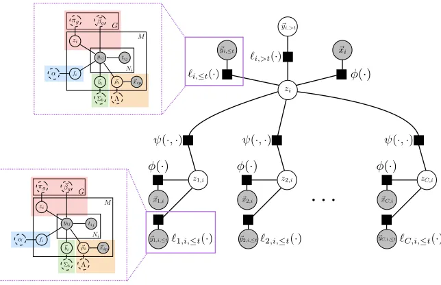
Figure 4: The factor graph of the coupled latent trajectory model. Empty nodes denote latent random variables, and shaded nodes denote observed variables. The latent trajectory model (LTM, described in Section 3.2) acts as a data-driven factor linking observed target and auxiliary marker histories into predictions.
3.4 Predicting Trajectories using the C-LTM
To predict trajectories (i.e. compute Eq. 1), we combine the LTM likelihood (Eq. 16), the LTM predictive (Eq. 24), and the coupling model (Eq. 25). Let`i,≤t(zi) stand as shorthand
for logp(~yi,≤t | zi, ~xi) and `ci,≤t(zc,i) stand as shorthand for logp(~yci,≤t | zci, ~xi), then we
see that
D(i, t)∝X
zi
p(y(·)|zi, ~yi,≤t, ~xi) X
z1:C,i
u(zi, z1:C,i| H(i, t)), (26)
where we have defined H(i, t) to be the set of information contained in the clinical history of individual i at time t: {~yi,≤t, ~y1:C,i,≤t, ~xi}, and used u(zi, z1:C,i | H(i, t)) to denote the
following unnormalized weight assigned to all values of the latent variables given the history:
u(zi, z1:C,i| H(i, t)),
exp (
`i,≤t(zi) +θ>f(zi, ~xi) + C X
c=1
`ci,≤t(zci) +θc>fc(zci, ~xi) +η>cgc(zi, zci) )
, (27)
To make D(i, t) a proper distribution, we normalizeu(zi, z1:C,i| H(i, t)) to obtain
p(zi| H(i, t)) = P
z1:Cu(zi, z1:C | H(i, t))
P z
P
z1:Cu(z, z1:C | H(i, t))
, Z
0 i,t(zi)
Zi,t
then we can writeD(i, t) (Eq. 1) as
D(i, t) =X
zi
p(y(·)|zi, ~yi,≤t, ~xi)p(zi| H(i, t)). (29)
Intuitively, we see that the predictive distribution under C-LTM is simply a weighted com-bination of the subtype-specific predictive distributions under LTM (Eq. 24). Moreover, the distribution p(zi | H(i, t)) is the marginal distribution over zi in a conditional random
field with structure similar to the coupling model (Eq. 25) but augmented with additional singleton factors defined by the LTM likelihood functions given the marker trajectory his-tories. The LTM likelihood factors in Eq. 27 are added into the model unchanged, but additional parameters {γ, γ1:C} can be included to reweight those terms (a similar idea is
used in Raina et al. (2003)).1 The factor graph for this conditional random field is shown in Figure 4. Note that the weight p(zi | H(i, t)) can be efficiently computed in time linear
in the number of auxiliary markers using the junction tree algorithm.
The C-LTM offers a number of advantages for predictive modeling of disease trajectories in domains where many other related marker trajectories are available. First, it allows irregularly and sparsely sampled trajectories to be neatly summarized using modularized, single-marker generative models. These can capture important latent factors and account for marker-specific measurement models and noise processes. Second, we can discriminatively
use auxiliary marker trajectory histories when modeling Eq. 1 instead of specifying a
joint generative model, which sidesteps the challenges associated with correctly specifying dependencies between many different marker types. Finally, the model can be used in continuous time and it dynamically updates predictions as new observations arrive.
3.5 Learning the C-LTM
We have described two components of our approach: the Latent Trajectory Model (LTM) and the coupling model. When these components are combined as shown in Section 3.4, then we obtain the C-LTM. The C-LTM has two conceptually distinct sets of parameters. The first set are those belonging to the individually trained LTMs for each marker type. To learn these, we can use the EM algorithm described in Schulam and Saria (2015). To learn the parameters for the C-LTM, we keep the single-marker model parameters fixed (e.g. those learned for the LTM), and use a standard gradient-based CRF learning algorithm (as described in Section 3.1.2) to optimize the penalized log-likelihood of example trajectory predictions. For completeness, we provide additional details for both stages in Appendix A.
3.5.1 Scalability
The EM algorithm used to learn the parameters of the LTM poses no serious challenges to scalability. The primary computational burden lies in the E-step wherein sufficient statistics from all individuals are computed and collected. This is linear in the number of patient records being analyzed, but since the inference required to compute the sufficient statistics can be performed independently for each individual given the current parameter estimates, the E-step can be easily parallelized to offset slow learning due to large numbers
of patient records. For any given individual, the E-step is dominated by the inversion of theNi×Ni covariance matrix. We do not expect this to be problematic, however, because
clinical markers in chronic diseases are observed at a maximum rate of 12 times per year. Moreover, such diseases occur over periods on the order of tens of years. Therefore, the number of measurements will be at most on the order of 100-200.
Learning the parameters of the CRF requires a sweep through all M|T | training in-stances in order to compute and aggregate the gradient at each iteration. The primary computational burden is computing the expected values of the features (Eq. 42), however, the tree-structured graphical model shown in Figure 4 allows the junction tree algorithm to run in time linear in the number of auxiliary markers. On a standard laptop, we are able to train the model on 772 patients (5,458 PFVC measurements) in 10-20 minutes.
Online inference for predicting a given individual’s future trajectory is also computation-ally straightforward. The key quantities are (1) the weightsp(zi| H(i, t)) in Eq. 29, which
are easily computed using the junction tree algorithm in time linear in the number of aux-iliary markers, and (2) the subtype-specific predictive densities p(y(·) |zi, ~yi,≤t, ~xi), which
have the same computational complexity as the E-step in the LTM learning algorithm.
4. Experiments
We demonstrate our approach by building a tool for predicting lung disease trajectories for individuals with scleroderma. Lung disease is currently the leading cause of death among scleroderma patients, and is notoriously difficult to treat due to the lack of accurate predictors of decline and tremendous variability across individual trajectories (Allanore et al., 2015). Clinicians use percent of predicted forced vital capacity (PFVC) to track lung severity, which is expected to drop as the disease progresses. In addition, they collect demographic information and other clinical marker values that measure the impact of disease on the different organ systems involved in scleroderma.
Data description. We train and validate our model using data from the Johns Hopkins Scleroderma Center patient registry, one of largest collections of clinical scleroderma data in the world. Demographic information is collected during the patient’s first visit to the clinic. PFVC and other clinical markers are collected during routine visits thereafter. To select individuals from the registry, we used the following criteria. First, we include individuals who were seen at the clinic within two years of their earliest scleroderma-related symptom2 (1,186 individuals). Second, we exclude all individuals with fewer than two PFVC measure-ments after first being seen by the clinic (398 individuals). Finally, we exclude individuals who received a lung transplant (16 individuals) because their natural trajectory is altered by the intervention. Transplants are rare so removing patients with transplants should not introduce significant bias. As mentioned earlier, there are no other known course-altering therapies for scleroderma.
Our final data set contains 772 individuals and a total of 5,458 PFVC measurements tracking individuals over a period of 20 years. The first, second, and third quartiles of the total number of PFVC measurements for an individual are 3, 5, and 9 respectively. The maximum number of PFVC measurements for one individual is 63. The first, second, and third quartiles of the measurement times are 1 year, 2.8 years, and 5.9 years. The first,
second, and third quartiles of elapsed time between measurements are 0.4 years, 0.7 years, and 1.10 years. The minimum and maximum elapsed time is 0.002 years and 16.4 years respectively.
The baseline demographic information includes gender and African American race, both of which have been shown to be associated with disease severity in scleroderma (Allanore et al., 2015). Antibody data are also collected at baseline, but since these are only available for a small subset of individuals, we do not include that data here. For time-dependent predictors, we include 5 auxiliary clinical markers. Three of the auxiliary markers are similar to PFVC in that they are continuous-valued test results used to measure the health of organ systems. We include: percent of predicted forced expiratory volume in one second (PFEV1), which measures the force with which air is expelled from the lungs; percent of predicted diffusing capacity (PDLCO), which measures the efficiency of oxygen diffusion from the lungs to the bloodstream; and total skin score (TSS), which is a cumulative measure of the thickness of the skin at various points on the body. In addition, we include 2 severity scores—clinical Likert-scaled judgements of organ damage severity: Raynaud’s phenomenon (RP) severity score, which measures the severity of damage to the extremities by issues related to the vasculature, and GI severity score that measures the severity of damage to the GI tract. For the interested reader, a more detailed discussion of these markers and their relationship to the disease can be found in Varga et al. (2012).
Experimental setup. For the 4 continuous-valued clinical markers (PFVC, PFEV1, PDLCO, TSS) we use the LTM and for the 2 severity scores (GI and RP) we use a simpler model that we will describe later. For the population model, we use constant functions (i.e. the basis expansion Φp(t) contains an intercept term whose coefficient is determined
by baseline covariates). For the subpopulation B-splines, we set boundary knots at 0 and 25 years (the maximum observation time in our data set is 23 years), use two interior knots that divide the time period from 0-25 years into three equally spaced chunks, and use quadratics as the piecewise components. For the individual-specific long-term basis Φ`, we use the
same basis as the population model (constant functions).
We divide our data into 10 folds and use log-likelihood on the first fold for tuning hyperparameters. For PFVC, we selectG= 9 subtypes using BIC. For the kernel hyperpa-rameters Θ1 ={Σb, α, `, σ2} we set Σb ∈R to be 16.0, which corresponds to the variance of individual-specific intercepts. We set α = 6,`= 2, and σ2 = 1 using a grid search over values chosen using domain knowledge. Qualitatively, these make sense; we expect transient
deviations to last around 2 years and to change PFVC by around ±6 units. Finally, we
penalize the expected log-likelihood with respect to β1:~ G as in Eq. 4 and set the weight
with anL1 regularizer. We optimize the objective using the Orthant-Wise Limited-memory Quasi-Newton (OWL-QN) algorithm (Andrew and Gao, 2007). To generate training examples for the C-LTM, we use times T ={1,2,4} (the first three quintiles of observation times in our data) to fit three different models. We choose time points earlier in the disease course because this is when it is most valuable to leverage all available information. In our cross-validated experimental results below, we estimate the penalty of theL1 regularization term in each fold by splitting a portion of the training data into a development set. We sweep the penalty from 1.0×10⁻⁷ to 1.0×10⁻¹ and choose based on development set performance.
Baselines. As a first baseline, we fit a regression model using static predictors only (features in~xi). This is to compare against typical approaches in clinical prediction which
rely only on observed features to predict disease progression (e.g. Khanna et al. 2011). The regression function is as follows, where Φ(t) is a B-spline basis:
ˆ
y(t)|~xi= Φ(t)>
~
β0+Pxijin~xixij
~
βi+Pxij,xikin pairs of~xixijxik
~ βij
. (30)
The following baselines reflect state-of-the-art approaches for dynamical prediction. The focus for each of these models, as discussed in the related work section, is on dynamical prediction of single marker trajectories using the marker history and static measurements collected during the first visit. The second baseline, like Rizopoulos (2011) and Shi et al. (2012), defines a single mean function parameterized in the same way as the first baseline and models individual-specific variations using a GP with the same kernel as in Equation 15 (using hyper-parameters as above). The third baseline is a mixture of B-splines, which models subpopulations that can express different trajectory shapes (as in Proust-Lima et al. (2014)).3 Finally, we use the LTM (no coupling to auxiliary markers) as a baseline. All B-spline bases used in these baseline models are parameterized in the same way as the C-LTM (described above).
Evaluation. Prediction accuracy for all models is measured using the absolute error between the predicted and a smoothed version of the individual’s observed trajectory. We make predictions after one, two, and four years of follow-up, which are summarized using averages computed in the second year of follow-up (t ∈ (1,2]), in the third and fourth year of follow-up (t∈ (2,4]), fifth to eighth year of follow-up (t∈ (4,8]), and beyond the eighth year of follow-up (t ∈ (8,25])4. Mean absolute errors (MAE) and standard errors
are estimated using 9-fold CV5 at the level of individuals (i.e. all of an individual’s data is held-out). Significance tests are computed against baselines using a paired t-test with point-wise predictions aggregated across folds.
4.1 Results
In this section, we present four sets of results. The first two are qualitative, and demon-strate the advantages of the C-LTM over the baseline models using examples. In the first
3. For the B-spline mixture, we use the subtypes discovered by LTM as the mixture classes. Without accounting for individual-specific variability explicitly, we have found that fitting a B-spline mixture using EM recovers poor classes that do not capture important trajectory shapes in the data. For additional details, see Section 3 in the supplement of Schulam and Saria (2015).
1 2 4 ● ● ● ● ●● ● ●●● ● ● ● ● ●●● ● ● ● ● ● ● ● ● ● ● ● ●● ● ●●● ● ● ● ● ●●● ● ● ● ● ● ● ● ● ● ● ● ●● ● ●●● ● ● ● ● ●●● ● ● ● ● ● ● ● 20 40 60 80 100
0.0 2.5 5.0 7.5 10.0 0.0 2.5 5.0 7.5 10.0 0.0 2.5 5.0 7.5 10.0 (a)
Pr( ) = Pr( ) =0.66 0.33
Pr( ) = Pr( ) =0.39 0.30
Pr( ) = Pr( ) =0.58 0.32
1 2 4
● ● ● ● ●● ● ●●● ● ● ● ● ●●● ● ● ● ● ● ● ● ● ● ● ● ●● ● ●●● ● ● ● ● ●●● ● ● ● ● ● ● ● ● ● ● ● ●● ● ●●● ● ● ● ● ●●● ● ● ● ● ● ● ● 20 40 60 80 100
0.0 2.5 5.0 7.5 10.0 0.0 2.5 5.0 7.5 10.0 0.0 2.5 5.0 7.5 10.0
1 2 4
● ● ● ● ●● ● ●●● ● ● ● ● ●●● ● ● ● ● ● ● ● ● ● ● ● ●● ● ●●● ● ● ● ● ●●● ● ● ● ● ● ● ● ● ● ● ● ●● ● ●●● ● ● ● ● ●●● ● ● ● ● ● ● ● 20 40 60 80 100
0.0 2.5 5.0 7.5 10.0 0.0 2.5 5.0 7.5 10.0 0.0 2.5 5.0 7.5 10.0
Years Since First Seen (b) (c) % P re di ct ed F orc ed V it al Ca pa ci ty (P F V C)
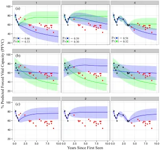
Figure 5: Examples of predictions made using 1, 2, and 4 years of data (moving across columns from left to right). Plot (a) shows dynamic predictions using C-LTM. Red markers are unobserved. Blue shows the trajectory predicted using the most likely subtype, and green shows the second most likely. Plot (b) shows dynamic predictions for the B-spline mixture baseline. Plot (c) shows the same for the B-spline + GP baseline.
qualitative analysis, we compare predictions made by C-LTM to those made by the B-spline mixture and the B-spline + GP. In the second qualitative analysis, we compare the C-LTM inferences with those from the LTM, which is a state-of-the-art single-marker model. The second two results are quantitative. The first compares predictive accuracies between the baseline models and the C-LTM. The second investigates clinical utility by using each model to predict a severity score that we use to detect individuals with aggressive lung disease.
4.1.1 Visual Comparison to Baselines
As an illustrative example to compare C-LTM with baselines, in Figures 5a, 5b, and 5c we show the dynamic predictions made using the C-LTM, the B-spline mixture, and the
B-spline + GP baselines on a sample patient.6 For each model, we show 95% posterior
intervals for the future trajectory. For the C-LTM and B-spline mixture, the most likely subtype is shown in blue and the second most likely is in green. The B-spline mixture (Figure 5b) cannot explain individual-specific sources of variation (e.g. short-term deviations from the mixture mean) and so over-reacts to the slight rise in PFVC seen in the last two observed (black) measurements in the second panel (year 2). The B-spline + GP (Figure 5c) cannot capture long-term differences in trajectory means (e.g. due to subtypes) and so pulls back to the population mean over time even after four years of data suggest a declining trajectory. On the other hand, at year 1 the C-LTM (Figure 5a) maintains the hypothesis that the individual may decline or return to stability (correctly putting most weight on the former). After 2 years of data, the temporary recovery seems to have caused confidence in the declining trajectory to fall (going from 66% to 39%), but the top-weighted hypothesis is still correct. After 4 years of data, the model again becomes confident in the declining trajectory. Clinically, this robustness to short-term changes is important. After having seen the recovery between years 1 and 2, a clinician may become less immediately concerned with the individual’s future lung disease, possibly delaying immunotherapy until a rapid decline becomes more evident. Note that the B-spline mixture, on the other hand, over-reacts to the recovery and predicts that the individual will continue to recover.
4.1.2 Analysis of Example Inferences
In Figure 6a-d, we show the C-LTM’s target and auxiliary marker inferences for four dif-ferent patients. For the target marker (PFVC) and auxiliary markers (TSS, PDLCO, and PFEV1), we show the most likely (blue) and second most likely (green) subtype and their corresponding trajectories. For the RP and GI severity score markers, we show the most likely severity class (high versus low). The dashed lines indicate the threshold at which high and low are determined based on judgements by our clinical collaborators. For PFVC, PFEV1, and PDLCO lower values indicate more severe progression. For TSS, higher values indicate severe progression. In Figures 6e-h, we show the predictions made by LTM to visually compare against predictions made using the baseline markers and PFVC history only (i.e. that do not leverage information from auxiliary markers).
● ● ● ● ● ● ● ● ● ● ● ● 20 40 60 80 100
0.0 2.5 5.0 7.5 10.0 Years Seen PFVC ●● ● ● ● ●● ● ● ●● ● 20 40 60 80 100
0.0 2.5 5.0 7.5 10.0
Years Seen PFVC ● ●● ● ● ●● ● ● ● ● ● ●●●● ●● 0 10 20 30 40 50
0.0 2.5 5.0 7.5 10.0
Years Seen TSS ● ● ●● ● ● ● ●● ● ● ● 20 40 60 80 100
0.0 2.5 5.0 7.5 10.0
Years Seen PDLCO ● ● ●● ● ● ● ● ●● ● ● 20 40 60 80 100
0.0 2.5 5.0 7.5 10.0
Years Seen PFEV1 ●●●● ● ●● ●● ● ● ●●●● ● ● ● low 0 40 80 120
0.0 2.5 5.0 7.5 10.0
Years Seen RP ●●● ● ● ● ● ● ● ● ● ●● ● ● ● ● ● low 0 40 80 120
0.0 2.5 5.0 7.5 10.0
Years Seen GI ●●● ● ● ● ●● ● ● ● ● ● ●● ● ●●● ● ●● ● ● ● ● ● ● ● 25 50 75 100
0 5 10 15
Years Seen PFVC ●●● ● ● ● ●●● ●● ● ● ●● ● ●● ●●●● ● ● ● ● ● ● ● 25 50 75 100
0 5 10 15
Years Seen PFVC ● ● ● ● ● ● ●● ● 0 10 20 30 40 50
0 5 10 15
Years Seen TSS ● ● ● ● ● ● ●● ●● ● ● ● ● ● ● ● ● ● ● ● ● ● ●● ● ● ● ● ● ● 25 50 75 100
0 5 10 15
Years Seen PDLCO ●●● ● ● ● ●●● ●●●● ●● ● ●● ●● ●● ● ● ●●● ● ● 25 50 75 100
0 5 10 15
Years Seen PFEV1 ●● ● ● ●● ● ● ● ● ● low 0 40 80 120
0 5 10 15
Years Seen RP ●● ● ● ●● ●● ● ● ● low 0 40 80 120
0 5 10 15
Years Seen GI (a) (b) (e) (f) ● ●●● ●● ● ● ● ● ● ● ● ● ● ●● ● 30 60 90
0 3 6 9
Years Seen PFVC ●●● ● ●● ● ● ● ● ● ● ● ● ● ●● ● 30 60 90
0 3 6 9
Years Seen PFVC ● ●● ● ● ● ● ●●●● ● ● ● 0 20 40
0 3 6 9
Years Seen TSS ● ●● ● ●● ● ● ● ●● ● ● ●● ●● ● 25 50 75
0 3 6 9
Years Seen PDLCO ● ●●● ●● ● ● ● ● ● ● ● ● ● ● ● ● 30 60 90
0 3 6 9
Years Seen PFEV1 ● ● ●● ● ● ● ● ● ● ● ●● ● high 0 40 80 120
0 3 6 9
Years Seen RP ● ● ●● ● ●●●●● ● ● ● ● low 0 40 80 120
0 3 6 9
Years Seen GI ● ● ● ● ●● ●● ● ● ● ● 30 60 90
0.0 2.5 5.0 7.5 10.0
Years Seen PFVC ● ● ● ● ●● ● ●●● ● ● 30 60 90
0.0 2.5 5.0 7.5 10.0 Years Seen PFVC ● ● ● ● ● ● ● ● ●● ● ● ● 0 20 40
0.0 2.5 5.0 7.5 10.0 Years Seen TSS ● ● ● ● ●● ● ●● ● ● 30 60 90
0.0 2.5 5.0 7.5 10.0 Years Seen PDLCO ● ● ● ● ● ● ● ● ●● ● ● 30 60 90
0.0 2.5 5.0 7.5 10.0 Years Seen PFEV1 ● ● ● ●●● ●● ● ● ● ● ● low 0 40 80 120
0.0 2.5 5.0 7.5 10.0 Years Seen RP ● ● ● ● ●● ●● ● ● ● ● ● high 0 40 80 120
0.0 2.5 5.0 7.5 10.0 Years Seen GI (c) (d) (g) (h)
C-LTM
LTM
In Figure 6b, we see a 75 year-old white woman who presents with healthy lung function (approximately 85 PFVC), but is consistently declining over the course of the first year by nearly 15 PFVC. A clinical rule of thumb is that a drop in 10 PFVC over the course of a year warrants close monitoring for active lung disease. We see that LTM extrapolates this initial trend and predicts that this individual will continue to decline rapidly (Figure 6f). Just as in the previous example, however, the auxiliary markers paint a more complete picture of this individual. In the first few PFEV1 observations, we see that this decline is not quite as pronounced and the progression is predicted to be more mild. In PDLCO we see that oxygen is absorbed into the blood at healthy levels and also predicted to remain stable (although incorrectly in this case). Finally, C-LTM predicts that the RP and GI severity scores will remain low, which also supports the prediction that this woman will stabilize. Note that in this example C-LTM overestimates the course of PDLCO and TSS. Although the model still makes the correct prediction for PFVC in spite of this mistake, it highlights that the performance of our approach may be further improved with better auxiliary marker inferences. As research in systems biology yields new insights into modeling specific measurements more precisely, the modular architecture of C-LTM makes it possible to improve overall performance by incorporating improved versions of the target or auxiliary marker models.
In Figure 6c, we see a 76 year-old white woman that presents with healthy lung function (just under 90 PFVC), which also appears to be stable given the subsequent test result taken later that same year. The LTM predicts that this individual’s most likely course is to remain stable. From the PFEV1 trajectory, however, we see that there was a large initial loss in PFEV1, which, together with the unusually high skin score (TSS) suggests that this woman’s disease is active. The activity in the other organ systems allows the C-LTM to offset the stability seen in the first two PFVC measurements and correctly predict the consistently declining lung trajectory.
Finally, in Figure 6d, we see a 67 year-old African American man with mildly impaired lung function early in the disease course (around 75 PFVC) that seems to recover over the next one or two years to a healthier 85 PFVC. In Figure 6h, we see that the LTM predicts that a stable trajectory thereafter is likely. By considering other organ systems, however, we see that this man’s blood-oxygen diffusion is severely limited early in the disease course (nearly 25% of the predicted DLCO). Moreover, we see that the this individual’s Raynaud’s phenomenon severity score is high early on and correctly predicted to remain that way. The low PDLCO and high RP severity score point to active vasculature disease, which is hypothesized to cause late deterioration in lung function. We see that C-LTM correctly uses this evidence to predict an accurate disease trajectory.
4.1.3 Predictive Accuracy
Predictions using 1 year of data
Model (1,2] (2,4] (4,8] (8,25]
B-spline with Baseline Feats. 13.17 (0.43) 14.07 (0.61) 14.34 (0.65) 14.12 (1.04) B-spline + GP 5.57 (0.24) 8.40 (0.19) 10.88 (0.42) 11.74(0.76) B-spline Mixture 6.31 (0.22) 7.59 (0.36) 9.82(0.46) 13.77 (0.55) LTM 5.70 (0.30) 8.02 (0.41) 11.17 (0.72) 13.93 (0.67) C-LTM F♣♠5.12(0.20) F♣♠6.88(0.27) F♣♠9.95 (0.51) F13.70 (1.08)
Predictions using 2 years of data
B-spline with Baseline Feats. 14.07 (0.61) 14.34 (0.65) 14.12 (1.04)
B-spline + GP 6.51 (0.19) 9.79 (0.35) 10.95 (0.68)
B-spline Mixture 6.17 (0.29) 8.34 (0.36) 12.19 (0.48)
LTM 5.74 (0.29) 8.08 (0.37) 10.89(0.62)
C-LTM F♣♠5.58(0.34) F♣7.99(0.61) F11.27 (1.02) Predictions using 4 years of data
B-spline with Baseline Feats. 14.34 (0.65) 14.12 (1.04)
B-spline + GP 6.60 (0.24) 9.53 (0.56)
B-spline Mixture 6.00 (0.37) 10.11 (0.56)
LTM 4.88(0.28) 8.65 (0.59)
C-LTM F♣5.04 (0.42) F♣♠8.07(0.35)
Table 1: Mean absolute error of PFVC predictions for the spline with baseline features, the B-spline + GP, LTM, and C-LTM. Bold numbers indicate best performance across baseline models and proposed model. F indicates statistically significant improvement against the B-spline model with baseline features only using a paired t-test (α= 0.05). ♣ indi-cates statistical significance compared against the B-spline + GP. indicates statistical significance compared against the B-spline mixture. ♠ indicates statistical significance compared against LTM.
LTM, we see that C-LTM benefits from leveraging information from auxiliary markers. As more information is collected, both models are able to the individual and provide compara-ble predictions. The B-spline mixture is not acompara-ble to personalize beyond capturing long-term trends across subpopulations, so we see that it becomes less competitive compared to both C-LTM and LTM as more data are collected. Finally, the B-spline + GP cannot capture long-term trends specific to subpopulations (as we saw in Section 4.1.1), and so we see that it does poorly when making predictions.
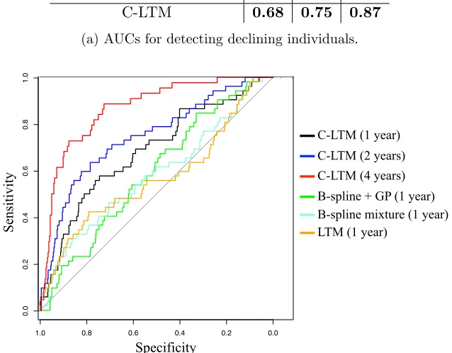
4.1.4 Clinical Utility
Model / Years of Data 1 2 4
B-spline + GP 0.59 0.63 0.74
B-spline mixture 0.58 0.63 0.76
LTM 0.57 0.71 0.84
C-LTM 0.68 0.75 0.87
(a) AUCs for detecting declining individuals.
Specificity
Sensitivity
0.0
0.2
0.4
0.6
0.8
1.0
1.0 0.8 0.6 0.4 0.2 0.0
Specificity
C-LTM (1 year) C-LTM (2 years) C-LTM (4 years) B-spline + GP (1 year)
LTM (1 year)
B-spline mixture (1 year)
Specificity
Sensitivity
0.0
0.2
0.4
0.6
0.8
1.0
1.0 0.8 0.6 0.4 0.2 0.0
Specificity
Sensitivity
0.0
0.2
0.4
0.6
0.8
1.0
1.0 0.8 0.6 0.4 0.2 0.0
S
ens
it
ivi
ty
(b) ROCs comparing B-spline + GP at 1 year, B-spline mixture at 1 year, LTM at 1 year, and C-LTM at years 1, 2, and 4.
Figure 7: Declining individual detection results.
are predicted to have active lung disease but do not, the results of the study are blurred because both arms of the trial may include many individuals without active lung disease.
and also includes the ROCs for the proposed model at years 2 (blue) and 4 (red) to visualize how performance improves as more data is added. Clinically, an AUC of 0.87 for predicting individuals with lung decline after—on average—four years of data is high and has not been shown previously.
5. Discussion
The goal of personalized (also called precision) medicine is to develop tools that help to tailor prognoses to the characteristics and unique medical history of the individual. In this paper, we describe an approach to personalized prognosis that uses an integrative analysis of multiple clinical marker histories from the individuals medical records. Our approach combines single-marker latent variable models (the LTM) with a CRF coupling model to make more accurate predictions about the future trajectory of a target clinical marker.
The coupled model (C-LTM) has several advantages. First, the marker-specific LTMs account for marker trajectory shapes using components at the population, subpopulation, individual long-term, and individual short-term levels, which simultaneously allows for het-erogeneity across and within individuals, and enables statistical strength to be shared across observations at different “resolutions” of the data. Within an individual marker model, the population and subpopulation components are learned offline, while estimates of the individual-specific parameters are refined over the course of the disease as data accrues for that individual. Second, our coupling model allows us to condition both the target and auxiliary marker histories to make predictions about the future target marker trajectory. We therefore use the marker-specific latent variable models to neatly summarize and ex-tra information from the irregularly sampled and sparse, while simultaneously sidestepping the issue of jointly modeling both the target and auxiliary markers. The conditional for-mulation is less sensitive to misspecified dependencies between different marker types and can also be easily scaled to diseases with a large number of auxiliary markers. Finally, our model aligns with clinical practice; predictions are dynamically updated in continuous time as new marker observations are measured. We also note that our description of the method and the experimental results focus on predicting the trajectory of a single clinical marker, but multiple latent factor regression models can be easily fit so that many markers can be simultaneously predicted. Using this extension, we only need to maintain different CRF parameters; the latent variable models are shared since they are fit independently as a precursor to learning the CRF.
latent factors may also be useful, but would make learning and inference in the latent factor CRF more challenging.
There are also several other immediate opportunities for improving the model. Aux-iliary markers are integrated via separate marker-specific generative models. While we incorporated two different types of models—trajectory and maximum-severity based—both of which were data driven, existing and new clinical knowledge should be brought to bear to improve these models, which we expect will improve predictions of the target trajectories. Further, in this work, we focused on modeling the dependency of the target subtype on the auxiliary markers. In addition, estimates of the individual-specific long-term and short-term components may also benefit from conditioning on the auxiliary markers. Finally, the parameters for the pairwise potentials learned in our model may serve as a means for generating hypotheses about the co-evolution of organ-specific trajectories.
The ideas proposed here also open up other longer-term directions for future work. The proposed model does not account for the effects of treatment on an individual’s long-term trajectory. In many chronic conditions, as is the case for scleroderma, drugs only provide short-term relief (accounted for in our model by the individual-specific adjustments). However, if treatments that alter long-term course are available and commonly prescribed, then these should be included within the model as an additional component that influences the trajectory. Learning these treatment effects from noisy electronic health record data (e.g., Xu et al. 2016) present an exciting and challenging direction for future work.
We have demonstrated our model by developing a prognostic tool for predicting lung disease trajectories in patients with scleroderma, an autoimmune disease. We showed that the proposed model makes more accurate predictions than state-of-the-art approaches. Ac-curate tools for prognosis can allow clinicians and patients to more actively manage their disease. While we have focused model development and evaluation on scleroderma, this work is broadly applicable to other complex diseases (Craig, 2008), many of which track disease activity using clinical scales of severity. The proposed model is most directly appli-cable to CCDs where heterogeneity in disease presentation is common. Examples of such diseases include lupus, multiple sclerosis, inflammatory bowel disease (IBD), chronic ob-structive pulmonary disease (COPD), and asthma. Extensions of the proposed ideas, and the model, to these diseases offer an opportunity to address important open challenges in precision medicine.
Acknowledgments