Gaussian Conditionally Markov Sequences: Theory with Application

(1)

University of New Orleans University of New Orleans

ScholarWorks@UNO

University of New Orleans Theses and

Dissertations Dissertations and Theses

Summer 8-5-2019

Gaussian Conditionally Markov Sequences: Theory with

Application

Reza Rezaie

University of New Orleans, [email protected]

Follow this and additional works at: https://scholarworks.uno.edu/td

Part of the Multi-Vehicle Systems and Air Traffic Control Commons, Navigation, Guidance, Control and Dynamics Commons, Signal Processing Commons, and the Systems and Communications Commons

Recommended Citation Recommended Citation

Rezaie, Reza, "Gaussian Conditionally Markov Sequences: Theory with Application" (2019). University of New Orleans Theses and Dissertations. 2679.

https://scholarworks.uno.edu/td/2679

This Dissertation is protected by copyright and/or related rights. It has been brought to you by ScholarWorks@UNO with permission from the rights-holder(s). You are free to use this Dissertation in any way that is permitted by the copyright and related rights legislation that applies to your use. For other uses you need to obtain permission from the rights-holder(s) directly, unless additional rights are indicated by a Creative Commons license in the record and/ or on the work itself.

(2)

Gaussian Conditionally Markov Sequences: Theory with Application

A Dissertation

Submitted to the Graduate Faculty of the University of New Orleans

in partial fulfillment of the requirements for the degree of

Doctor of Philosophy in

Engineering and Applied Science Electrical Engineering

by

Reza Rezaie

B.S. University of Kerman, 2006 M.S. Shiraz University, 2009

(3)

(4)

(5)

Acknowledgments

I would like to express my special appreciation and thanks to my advisor Professor X. Rong Li. I have learned a lot from him not only about my research, but also critical and independent thinking in general. He has been always very patient to discuss any topic in depth and generously share his thought and experience with me. He has always made time for me in his busy schedule. I will always remember beautiful moments we spent together.

I would like to express my sincere gratitude and thanks to Professor Vesselin P. Jilkov and Professor Huimin Chen for their invaluable comments on my work. Their critical comments have been very helpful to improve my work. My deepest thanks go to Professor Linxiong Li and Professor Kenneth Holladay for their useful classes and their insightful comments on my research. I really enjoyed their classes in the Department of Mathematics. I am also thankful to Professor Huimin Chen and Professor Linxiong Li, who have always made time for me despite being busy.

I would like to thank my lovely family for all their emotional support and help.

I am also grateful to all my wonderful friends and labmates who have been with me during my PhD.

(6)

Content

List of Figures . . . vii

Abbreviations . . . viii

Abstract . . . ix

1 Introduction . . . 1

1.1 Importance of this Research . . . 1

1.2 Existing Results and Our Contributions . . . 2

1.2.1 CM Processes in Theory and Application . . . 2

1.2.2 Chapter 2 . . . 3

1.2.3 Chapter 3 . . . 4

1.2.4 Chapter 4 . . . 6

1.2.5 Chapter 5 . . . 7

1.2.6 Chapter 6 . . . 8

1.2.7 Chapter 7 . . . 10

1.2.8 Conventions and Notations . . . 11

2 Modeling and Characterizing Nonsingular Gaussian CM Sequences . . . 13

2.1 Definitions and Preliminaries . . . 13

2.1.1 CM Definitions and Notations . . . 13

2.1.2 Preliminaries (for Gaussian CM Sequences) . . . 14

2.2 Dynamic Models of CMc Sequences . . . 16

2.3 Characterization ofCMc Sequences . . . 20

2.4 Dynamic Models of [k1, k2]-CMc Sequences . . . 22

3 Reciprocal Sequences from the CM Viewpoint. . . 25

3.1 Reciprocal Sequences . . . 25

3.1.1 Reciprocal Characterization from CM Viewpoint . . . 26

3.1.2 ReciprocalCMc Dynamic Models . . . 31

3.1.3 Recursive Estimation of Reciprocal Sequences . . . 33

3.2 Characterizations: Other CM Classes vs. Reciprocal . . . 34

3.2.1 CML∩[k1, N]-CMF . . . 34

3.2.2 CML∩[0, k2]-CML (CMF ∩[k1, N]-CMF) . . . 35

3.2.3 More About Intersections of CM Classes Relative to Reciprocal . . . 37

4 Models and Representations of Gaussian Reciprocal and Other Gaussian CM Sequences . . . 39

4.1 Dynamic Models of Reciprocal and Intersections of CM Classes . . . 39

4.1.1 Reciprocal Sequences . . . 39

4.1.2 Intersections of CM Classes . . . 43

(7)

5 Singular/Nonsingular Gaussian CM Sequences . . . 51

5.1 Dynamic Model and Characterization of CMc Sequences . . . 51

5.1.1 Dynamic Model . . . 51

5.1.2 Characterization . . . 54

5.2 Characterization and Dynamic Model of Reciprocal Sequences . . . 55

5.2.1 Characterization . . . 55

5.2.2 Dynamic Model . . . 56

5.3 Characterizations and Dynamic Models of Other CM Sequences . . . 57

6 Algebraically Equivalent Dynamic Models of Gaussian CM Sequences . . . 59

6.1 Preliminaries: Dynamic Models . . . 59

6.2 Determination of Algebraically Equivalent Models: A Unified Approach . . . 62

6.3 Algebraically Equivalent Models: Examples . . . 64

6.3.1 Forward and Backward Markov Models . . . 64

6.3.2 ReciprocalCML and Reciprocal Models . . . 65

6.4 More About Algebraically Equivalent Models . . . 66

6.4.1 Models Algebraically Equivalent to a Reciprocal Model . . . 66

6.4.2 Parameters of Equivalent Markov and Reciprocal Models . . . 69

6.5 Markov Models and Reciprocal/CML Models . . . 70

7 Trajectory Modeling, Filtering, and Prediction Using CM Sequences . . . . 72

7.1 DDT Modeling . . . 72

7.1.1 CML Sequences for DDT Modeling . . . 73

7.1.2 CML Model Parameter Design for DDT Modeling . . . 75

7.2 DDT Filtering . . . 76

7.2.1 First Formulation . . . 76

7.2.2 Second Formulation . . . 78

7.2.3 Discussion . . . 80

7.3 DDT Prediction . . . 81

7.4 Simulations . . . 84

8 Conclusions and Future Work . . . 98

Bibliography . . . .102

Appendix . . . .108

A Proof of Lemma 2.3.4 . . . 108

B (Probabilistically) Equivalent Models . . . 109

B.1 CML Sequences . . . 110

B.2 CMF Sequences . . . 111

B.3 Reciprocal Sequences . . . 113

B.4 Markov Sequences . . . 113

C Algebraically Equivalent Models . . . 114

C.1 Reciprocal Model and Markov Model . . . 114

C.2 CML Model and Markov Model . . . 114

C.3 CMF Model and Reciprocal Model . . . 115

C.4 CML Model and Backward CMF Model . . . 115

D Transition Density of a Markov-Induced CML Model . . . 115

(8)

List of Figures

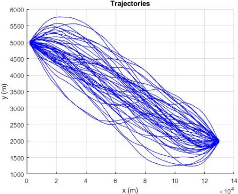
7.1 CML trajectories from an origin to a destination (Example 1, Scenario 1). . . 85

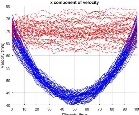
7.2 CML (solid lines) and Markov (dash lines) trajectories (Example 1, Scenario 1). 86 7.3 x-velocity forCML and Markov trajectories (Example 1, Scenario 1). . . 86

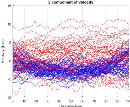
7.4 y-velocity forCML and Markov trajectories (Example 1, Scenario 1). . . 86

7.5 y-velocity forCML trajectories (Example 1, Scenario 1). . . 87

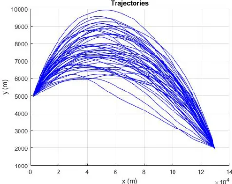
7.6 CML and Markov trajectories (Example 1, Scenario 2). . . 87

7.7 x-velocity forCML and Markov trajectories (Example 1, Scenario 2). . . 87

7.10 CML and Markov trajectories (Example 1, Scenario 3). . . 89

7.11 x-velocity forCML and Markov trajectories (Example 1, Scenario 3). . . 89

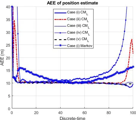
7.15 AEE of position estimate (AEEp_k_|_k) (Example 2). . . 92

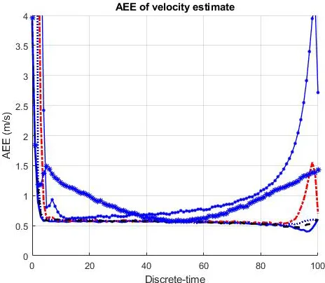
7.16 AEE of velocity estimate (AEEv_k_|_k) (Example 2). . . 93

7.17 Log of AEE of position predictions ofxN (AEEp_N|k) (Example 3). . . 94

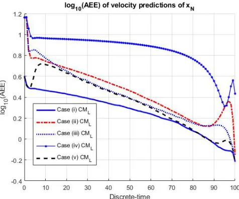
7.18 Log of AEE of velocity predictions ofxN (AEEv_N_|_k) (Example 3). . . 94

7.19 Log of AEE of position prediction (log₁₀(AEE9+n|9)) (Example 4). . . 95

7.20 CML trajectories from an origin to a destination (Example 5). . . 96

7.21 CML and Markov trajectories (Example 5). . . 96

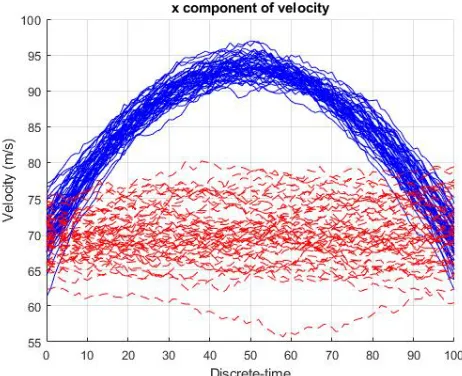
7.22 x-velocity forCML and Markov trajectories (Example 5). . . 96

(9)

Abbreviations

a.s. almost surely

CM conditionally Markov

NG nonsingular Gaussian

ZMG zero-mean Gaussian

(10)

Abstract

Markov processes have been widely studied and used for modeling problems. A Markov process has two main components (i.e., an evolution law and an initial distribution). Markov processes are not suitable for modeling some problems, for example, the problem of predicting a trajectory with a known destination. Such a problem has three main components: an origin, an evolution law, and a destination. The conditionally Markov (CM) process is a powerful mathematical tool for generalizing the Markov process. One class of CM processes, calledCML, fits the above components of trajectories with a destination. The CM process combines the Markov property and conditioning. The CM process has various classes that are more general and powerful than the Markov process, are useful for modeling various problems, and possess many Markov-like attractive properties.

Reciprocal processes were introduced in connection to a problem in quantum mechanics and have been studied for years. But the existing viewpoint for studying reciprocal processes is not revealing and may lead to complicated results which are not necessarily easy to apply.

We define and study various classes of Gaussian CM sequences, obtain their models and characterizations, study their relationships, demonstrate their applications, and provide general guidelines for applying Gaussian CM sequences. We develop various results about Gaussian CM sequences to provide a foundation and tools for general application of Gaussian CM sequences including trajectory modeling and prediction.

We initiate the CM viewpoint to study reciprocal processes, demonstrate its significance, obtain simple and easy to apply results for Gaussian reciprocal sequences, and recommend studying reciprocal processes from the CM viewpoint. For example, we present a relationship between CM and reciprocal processes that provides a foundation for studying reciprocal pro-cesses from the CM viewpoint. Then, we obtain a model for nonsingular Gaussian reciprocal sequences with white dynamic noise, which is easy to apply. Also, this model is extended to the case of singular sequences and its application is demonstrated. A model for singular sequences has not been possible for years based on the existing viewpoint for studying reciprocal processes. This demonstrates the significance of studying reciprocal processes from the CM viewpoint.

(11)

Chapter 1

Introduction

1.1 Importance of this Research

For modeling a problem in probability theory, usually the following order should be considered [1]. First, if the problem is time-invariant, a random variable might be good enough. Otherwise, a stochastic process seems necessary. An independent process can be considered first for its simplicity. If such a simple process is not good enough, the next choice is usually a Markov process. A Markov process has two elements (an evolution law and an initial distribution). However, even the Markov process is not good enough for some problems. Then, sometimes a higher order (e.g., second order) Markov process is used. But such a model does not fit some problems well, for example, a time-varying problem with some information available about its future (e.g., destination). More specifically, consider the problem of predicting a trajectory with known destination. Such a problem in, e.g., air traffic control (ATC), has three elements: an origin, an evolution law, and a destination, to which the Markov process does not fit since it can not account for the destination information. In fact, the destination distribution of a Markov process is completely determined by its initial distribution and evolution law. The conditionally Markov (CM) process is a powerful mathematical tool for generalizing the Markov process. One class of CM processes calledCMLhas the following elements: an evolution law and a joint distribution of the two endpoints (i.e., an initial distribution and a destination distribution conditioned on the initial). The CML process can model destination information and has a Markov-like evolution law, which is powerful and simple. The CML process is more suitable than the Markov process for modeling problems with destination information. For example, it can be used in ATC for trajectory modeling, prediction, and conflict detection.

Conditioning is a very powerful tool in probability theory. The Bayes rule follows from the definition of conditional probability. The concept of posterior probability, which relies on the concept of conditioning, is essential in probability and statistical inference. Conditioning is the key idea in the total probability theorem, which is extremely useful for many problems. The Markov property, being very important and widely used, is based on conditioning. The CM process combines the Markov property and conditioning. Different ways of combining the two lead to different classes of CM processes, which are more general and powerful than the Markov process. The CM process has various classes that are more general and powerful than the Markov process, are useful for modeling various problems, and possess many Markov-like attractive properties. CM processes are important for problem modeling and should be studied in order to provide useful results for their application. We define and study various classes of CM processes, obtain their dynamic models and characterizations, study their relationships, demonstrate their applications, and provide general guidelines for using CM processes in application.

(12)

its power, obtain simple and easy to apply results for reciprocal processes, and recommend studying reciprocal processes from the CM viewpoint.

1.2 Existing Results and Our Contributions

Consider stochastic sequences1 defined over [0, N] = {0,1, . . . , N}. For convenience, let the index be time. A sequence is Markov if and only if (iff) conditioned on the state at any time k, the segment before k is independent of the segment after k. A sequence is reciprocal iff conditioned on the states at any two timesk1 andk2, the segment inside the interval (k1, k2) is

independent of the segments outside [k1, k2]. In other words, inside and outside are independent

given the boundaries. A sequence is CM over [k1, k2]2 iff conditioned on the state at time k1

(k2), the sequence is Markov over [k1+ 1, k2] ([k1, k2−1]). Therefore, there are several classes

of CM sequences with differentk1,k2, and the conditioning time (i.e., conditioning at the first

or the last time of the CM interval). So, the set of CM sequences is very large and its two important special classes are the Markov sequence and the reciprocal sequence.

Markov processes have been widely studied and used for modeling problems. However, they are not general enough in some cases [36]–[51], and more general processes are needed. The reciprocal process is a generalization of the Markov process. The CM process is a powerful mathematical tool for generalizing the Markov process.

In this chapter, we review existing results and our contributions in each chapter of the dissertation. In Chapter 2 to Chapter 6, we present results about CM sequences. We also point out applications of different classes of CM sequences. In Chapter 7, an application of CM sequences in trajectory modeling is discussed in more detail. First, we present a general overview of CM processes in theory and application.

1.2.1 CM Processes in Theory and Application

The CM process is a very large class of stochastic processes with various classes defined based on the Markov property and the conditioning. Some classes of Gaussian CM processes were defined in [52] based on mean and covariance functions, and later studied further in [29]. CM processes are powerful in both theory and application. However, their power has not been appreciated in the literature, and their study is limited to the above two papers. We demonstrate the power of CM processes (the CM property) in theory and application.

Reciprocal processes have been widely studied and used in various fields/problems, e.g., ap-plied mathematics, theoretical physics, stochastic mechanics, image processing, intent inference, and acausal systems [2]–[51]. In these papers, reciprocal processes were defined, their proper-ties were studied, their dynamic models were presented, their estimation was addressed, their importance and usefulness were demonstrated, and their applications in various problems were discussed. Reciprocal processes include the Markov process as a special case. The properties, models, and estimators of reciprocal processes presented in the literature are much more com-plicated than those of Markov processes. In essence, the literature studies the reciprocal process from inside the set (of reciprocal processes) without paying attention to processes outside. As we show later, this viewpoint may lead to complicated results and difficulties. Also, it does not reveal some hidden properties of the reciprocal process. Fortunately, as we demonstrate later, CM processes (including the reciprocal process) can provide an alternative and in fact better viewpoint for studying reciprocal processes with many benefits. From the CM viewpoint we can study the reciprocal process from outside of the set as well. This viewpoint gives a clearer picture of the reciprocal process, is more revealing, and leads to simpler results. This

demon-1_{Our definitions and some of our results work for both discrete index and continuous index processes; however,}

we present them all for discrete index processes (i.e., sequences).

(13)

strates the power of CM processes in theory. However, the literature on the reciprocal process has not appreciated its relationship to the CM process and has not recognized the significance of studying the reciprocal process from the CM viewpoint. Only very few papers implicitly benefited from the CM property [30]–[31]. For example, as we show later, studying reciprocal sequences from the CM viewpoint is very insightful and fruitful. But there is no paper in the literature on studying reciprocal sequences from the CM viewpoint.

CM processes are powerful and flexible for modeling complicated problems (systems/ phe-nomena), where Markov processes are not adequate. The CM property is based on the Markov property and the conditioning. Different ways of combining the two give different CM classes. As we illustrate later, by an appropriate combination of the Markov property and the condi-tioning we can define a suitable CM process for modeling a given problem. The power of CM processes for problem modeling has not been recognized in the literature. We develop a theoret-ical foundation of (Gaussian) CM sequences/processes, obtain results/tools (properties, models, characterizations, representations, etc.) for their application, present guidelines for their use in problem modeling, and demonstrate their application. For example, we demonstrate an applica-tion of CML sequences to trajectory modeling with destination information. Some papers used (finite state) reciprocal sequences, which are specialCML sequences, for modeling such trajec-tories [41]–[47]. CML sequences and the structure of their dynamic model provide a natural, simpler, and more general framework for modeling trajectories with destination information. However, they have not been used in the literature.

1.2.2 Chapter 2

The notion of Gaussian CM processes was introduced in [52] based on mean and covariance functions of Gaussian processes. [52] studied and characterized continuous time stationary Gaussian CM processes that are nonsingular on the interior of the time interval. [29] extended the definition of Gaussian CM processes (in [52]) to the general (Gaussian/nonGaussian) case. Furthermore, [29] commented on some properties of Gaussian CM processes and Gaussian recip-rocal processes. By conditioning on the state of the process at the first time of the CM interval, different Gaussian CM processes were defined in [52]. However, it is possible not only to extend the definitions to non-Gaussian processes, but also to other CM processes by conditioning on the state at the last time of the CM interval. Such processes are useful for both theory and application. Despite their power in theory and application, to our knowledge, (unlike reciprocal processes) CM processes have not received much attention and have not been studied well to gain understanding and to obtain tools for application. In addition, the literature on the recip-rocal process has not appreciated its relationship to the CM process well and has not benefited from it except implicitly in very few cases [30]–[31]. In particular, we are not aware of any paper studying Gaussian reciprocal sequences from the CM viewpoint.

The main goal of Chapter 2 is two-fold: 1) to define and study various useful classes of CM sequences and provide useful and easy to apply results for their application, e.g., for motion trajectory modeling with destination information, and 2) to lay a foundation for studying an important special class of CM sequences, the reciprocal sequence, from the CM viewpoint.

(14)

and backward dynamic models of (stationary/non-stationary) nonsingular Gaussian (NG) CM sequences in a recursive form are obtained. These models are complete descriptions of the corresponding classes of NG CM sequences. Based on the models, characterizations of NG CM sequences are obtained. As a by-product, new factorizations of two covariance matrices, characterizing two classes of NG CM sequences, are presented.

From system theory, it is well known that the state concept is equivalent to the Markov property, that is, conditioned on the state at a time, the states before and after are independent. That is why there exists a simple recursive model for the evolution of the Markov sequence. However, for the general Gaussian sequence there is no simple recursive model for the evolution. The CM sequence is more general than the Markov sequence. Consequently, a CM sequence does not necessarily have the above concept of state, in general. Instead, it has a similar concept if it is conditioned at two instead of one time. That is why a simple recursive model also exists for the evolution of Gaussian CM sequences.

Part of the results presented in Chapter 2 have appeared in [53].

1.2.3 Chapter 3

Reciprocal processes have been used in many different areas of science and engineering (e.g., [36]–[51]) where stochastic processes more general than Markov processes are needed. [36]–[39] discussed reciprocal processes in the context of stochastic mechanics. In [40], the behavior of acausal systems was described using reciprocal processes. More specifically, on the one hand, re-ciprocal processes are a generalization of Markov processes. On the other hand, acausal systems can be seen as a generalization of causal systems [40]. Then, the relationship between acausal systems and reciprocal processes was studied in [40]. Also, Based on quantized state space, [41]–[46] used finite state reciprocal sequences for trajectory modeling, detection of anomalous trajectory pattern, intent inference, tracking, and track-before-detect. The idea of the reciprocal process was implicitly utilized in [48]–[49] for intent inference in vehicle’s intelligent interactive displays. Application of reciprocal processes in image processing was discussed in [50]–[51]. The behavior of particles in the problem posed in [3]–[4] by Schr¨odinger can be explained in the reciprocal process setting [2].

(15)

Despite many papers on the theory of reciprocal processes (e.g., [2], [5]–[35]), there is still a lack of easy to apply results/tools for their application. To make this issue clear and demonstrate the significance of studying reciprocal processes from the CM viewpoint, as an example, consider a dynamic model of NG reciprocal sequences presented in [18], which is the most significant paper on Gaussian reciprocal sequences. It was shown that the evolution of a NG reciprocal sequence can be described by a second-order nearest-neighbor model driven by locally correlated dynamic noise [18]. That model describes the NG reciprocal sequence completely (i.e., necessarily and sufficiently), and can be considered a natural generalization of the Markov model. However, due to its nearest neighbor structure and its colored dynamic noise, it is not easy to apply. Also, recursive estimation of a reciprocal sequence based on the model of [18] is challenging. That is why several papers [18], [32]–[35] tried to find a recursive estimator. Clearly, a simpler and easier to apply model for NG reciprocal sequences is desired. But it is difficult to derive such a model from the viewpoint of the existing literature including [18]. So, a simpler yet complete description of the NG reciprocal sequence in an alternative viewpoint is desired. CM sequences provide such a good viewpoint, leading to many benefits. In other words, the literature studies reciprocal sequences from inside the set of reciprocal sequences without paying attention to sequences outside. This viewpoint may lead to complicated results and difficulties. From the CM viewpoint, however, we can also study the reciprocal sequence from outside. The CM viewpoint gives a clearer picture of the reciprocal sequence (from outside), is more revealing, and leads to simple results. For example, we obtain a dynamic model with white dynamic noise for the NG reciprocal sequence from the CM viewpoint, based on which recursive estimation is straightforward.

The main goal of Chapter 3 is three-fold: 1) to propose studying reciprocal sequences from the CM viewpoint and demonstrate its significance, insightfulness, and fruitfulness, 2) to study NG reciprocal sequences from the CM viewpoint, 3) to obtain easy to apply results and tools for NG reciprocal sequences.

The main contributions of Chapter 3 are as follows. The reciprocal sequence is studied explicitly from the CM viewpoint, which is a larger set of sequences. Studying, modeling, and characterizing the reciprocal sequence from this viewpoint are different from those of [18] and the literature. This fruitful angle has several advantages. It provides more insight into the reciprocal sequence via its relationship to other CM sequences. As a result, new properties of the Gaussian reciprocal sequence are revealed. In addition, the CM sequence and the reciprocal sequence can be treated in the same way. This is not only theoretically interesting, but also useful for application. We demonstrate that the relationship between the Gaussian CM process and the Gaussian reciprocal process stated in [29] is incomplete. More specifically we elaborate on the comment of [29], show that the said relationship is not sufficient even for Gaussian processes, and obtain a relationship between the general (Gaussian/non-Gaussian) reciprocal and CM processes. A characterization of the NG reciprocal sequence is obtained based on its relationship to the CM sequence. This characterization is the same as that of [18], but it is obtained by a different approach and from a different viewpoint. We show that a NG sequence is reciprocal iff it is both CML (i.e., conditioned on the state at the last time N is Markov over [0, N −1]) and CMF (i.e., conditioned on the state at the first time 0 is Markov over [1, N]). In addition, we discuss how characterizations change from a NG CM sequence to the NG reciprocal sequence and then to the NG Markov sequence; that is, how different classes of NG CM sequences contribute to the construction of the NG reciprocal sequence, namely a spectrum of characterizations from a CM class to the reciprocal class. Moreover, we obtain new dynamic models for the NG reciprocal sequence based on the forward and backward models of CMLand CMF sequences. We call these models reciprocalCML and reciprocalCMF models. They are driven by white (rather than colored) noise and are easy to apply. Also, we discuss under what conditions these models are for NG Markov sequences.

(16)

1.2.4 Chapter 4

Due to its simple structure and whiteness of the dynamic noise, our reciprocal CML model is easy to apply, e.g., for trajectory modeling with destination. For example, recursive estimation of a reciprocal sequence based on a reciprocal CML model is straightforward. However, it is not clear how parameters of a reciprocal CML model can be designed in a problem. More generally, aCMLsequence and its dynamic model (obtained in Chapter 2) can model trajectories with destination. However, guidelines for parameter design of a CML model are required. Following [9], [43] used a transition probability function of a finite state reciprocal sequence from a transition probability function of a finite state Markov sequence in a quantized state space for a problem of intent inference. But [43] did not discuss if all reciprocal transition probability functions can be obtained from a Markov transition probability function, which is critical for application. Also, it is not always feasible or easy to quantize the state space in some applications. NG Markov sequences modeled by the same reciprocal model of [18] were studied in [16]. However, the results are based on the model of [18], which is not simple or easy to apply.

The main goal of Chapter 4 is three-fold: 1) to present some approaches/guidelines for parameter design ofCML,CMF, and reciprocalCMLmodels for their application, 2) to obtain a representation of NG CML, CMF , and reciprocal sequences, revealing a key fact about these sequences, and to emphasize the significance of studying reciprocal sequences from the CM viewpoint, and 3) to present a full spectrum of dynamic models from a CML model to a reciprocal CML model and show how models of various intersections of CM classes can be obtained.

The main contributions of Chapter 4 are as follows. From the CM viewpoint, we not only show how a Markov model induces a reciprocalCMLmodel, but also prove thatevery reciprocal CML model can be induced by a Markov model. Then, we give formulas to obtain parameters of the reciprocalCMLmodel from those of the Markov model. This approach is more intuitive than a direct parameter design of a reciprocalCMLmodel, because one usually has an intuitive understanding of Markov models. A full spectrum of dynamic models from aCML model to a reciprocalCMLmodel is presented. This spectrum helps to understand the gradual change from aCMLmodel to a reciprocalCMLmodel. For application of other CM classes, e.g. intersection of two CM classes defined in Chapter 2, we need their dynamic models. It is demonstrated how dynamic models for intersections of NG CM sequences can be obtained. In addition to their usefulness for application, these models are particularly useful to describe the behavior of a sequence (e.g., a reciprocal sequence) belonging to more than one CM class. Based on a valuable observation, [29] discussed representations of NG continuous time CM processes (including NG continuous time reciprocal processes) in terms of a Wiener process and an uncorrelated NG vector. First, we show that the representation presented in [29] is not sufficient for a Gaussian process to be reciprocal (although [29] stated that the representation was sufficient, which has not been corrected so far). Then, we obtain a simple (necessary and sufficient) representation for NG reciprocal sequences from the CM viewpoint. As a result, the significance of studying reciprocal sequences from the CM viewpoint is demonstrated. Second, inspired by [29], we show that a NG CML (CMF) sequence can be represented by a sum of a NG Markov sequence and an uncorrelated NG vector. This (necessary and sufficient) representation makes a key fact of CM sequences clear and provides some insight for parameter design ofCML and CMF models based on those of a Markov model and an uncorrelated NG vector. Third, we study the obtained representations of NG CML, CMF, and reciprocal sequences in detail and, as a by-product, obtain new representations of some matrices, which are characterizations of NG CML, CMF, and reciprocal sequences.

(17)

1.2.5 Chapter 5

From the viewpoint of singularity, one can consider two extreme cases for Gaussian sequences. One extreme is a sequence being almost surely constant throughout the time interval. The other extreme is a nonsingular sequence, i.e., a sequence with a nonsingular covariance matrix. For example, a Gaussian sequence can be singular because it is almost surely constant over time or at a time (i.e., the state over time or at a time is almost surely constant), or because the states of the sequence at two or more times are almost surely linearly dependent. There are various such causes (corresponding to different times) leading to singular Gaussian sequences. As a result, we have various singularity. It is desired to model and characterize all singular and nonsingular Gaussian sequences in a unified way.

Characterizations of NG Markov, reciprocal, and CM sequences presented in [56], [18], Chap-ters 2, and Chapter 3 are based on the inverse of the covariance matrix of the whole sequence. So, they do not work for singular sequences. In [57] a characterization was presented for the scalar-valued (singular/nonsingular) Gaussian Markov process in terms of the covariance func-tion. However, that characterization does not work for the general vector-valued case. In [58] a characterization was presented for a special kind of NG reciprocal processes (i.e., second-order NG processes, that is, Gaussian processes with covariance matrices corresponding to any two times of the process being nonsingular) in terms of the covariance function of the process. [19] presented a characterization of the Gaussian reciprocal process based on the Markov prop-erty. That characterization is actually a representation of the reciprocal process in terms of the Markov process and is specifically for continuous time processes. [30] presented a different characterization of the Gaussian reciprocal process based on the Markov property. Characteriza-tions of [19] and [30] converted the question about a characterization of the Gaussian reciprocal process to the question about a characterization of the Gaussian Markov process, which was left unanswered for the general vector-valued Gaussian process. Later studies on the covariance of Gaussian processes were mainly under nonsingularity assumption [59]–[61]. Despite the above attempts, to our knowledge, there is no characterization in terms of the covariance function for the general (singular/nonsingular) Gaussian CM (including reciprocal and Markov) process in the literature.

The well-posedness of the reciprocal dynamic model presented in [18] (i.e., the uniqueness of the sequence obeying the model) is guaranteed by the nonsingularity assumption for the covariance of the whole sequence. It can be seen that unlike the model of [18], the nonsingularity assumption is not critical for the uniqueness of sequences obeying CM dynamic models presented in Chapter 2. Dynamic models of the NG reciprocal sequence obtained in Chapter 2 does not work for singular sequences, although the nonsingularity assumption is not critical for its well-posedness. To our knowledge, there is no dynamic model for the Gaussian reciprocal sequence3 in the literature. For example, it is not clear how the model of [18] can be extended to the Gaussian reciprocal sequence. More generally, there is no dynamic model for Gaussian CM sequences in the literature.

Although they make the analysis and modeling easy, nonsingularity assumptions restrict application of Gaussian CM (including reciprocal and Markov) sequences. Without such as-sumptions, we have a larger and more powerful set of sequences for modeling problems. Some problems can be modeled by a singular sequence better than a nonsingular one. For example, a NG CML sequence is used in Chapter 7 for trajectory modeling between an origin and a destination. Now assume that the origin/destination is known, i.e., some components of the state of the sequence at the origin/destination are almost surely constant. Then, a singular CML sequence is better for modeling such trajectories.

3

(18)

The main goal of Chapter 5 is threefold: 1) to obtain dynamic models and characteriza-tions of the general Gaussian CM sequence to unify singular and nonsingular Gaussian CM sequences theoretically, 2) to provide tools for application of (singular/nonsingular) Gaussian CM sequences, e.g., in trajectory modeling with destination information, 3) to emphasize the significance of studying reciprocal sequences from the CM viewpoint, e.g., by obtaining two dynamic models for the general Gaussian reciprocal sequence from the CM viewpoint.

The main contributions of Chapter 5 are as follows. Dynamic models and characterizations of (singular/nonsingular) Gaussian CM, reciprocal, and Markov sequences are obtained. Two types of characterizations are presented for Gaussian CM and reciprocal sequences. The first type is in terms of the covariance function of the sequence. The second type, which has a similar spirit to (but different from) those of [19] and [30], is based on the state concept in system theory (i.e., the Markov property). Then, by deriving a characterization for the general vector-valued Gaussian Markov sequence in terms of the covariance function, we can check the Markov property. Then, the second type of characterization of Gaussian CM and reciprocal sequences becomes complete and makes a better sense. It is shown that dynamic models of Gaussian CM sequences have a structure similar to those of NG CM sequences presented in Chapter 2, and the difference is in the values of their parameters. Therefore, the presented models unify singular and nonsingular CM sequences. We obtain two dynamic models for the Gaussian reciprocal sequence from the CM viewpoint. As a result, the significance and the fruitfulness of studying reciprocal sequences from the CM viewpoint is demonstrated. A full spectrum of models (characterizations) ranging from a CML model (characterization) to a reciprocalCML model (characterization) for Gaussian sequences is presented. The obtained models and characterizations unify singular and nonsingular Gaussian CM sequences. The representation of NG CML/CMF sequences presented in Chapter 4 is extended to the general singular/nonsingular Gaussian case.

1.2.6 Chapter 6

The evolution of a Markov sequence can be modeled by a Markov, reciprocal, CML, or CMF model4. Similarly, the evolution of a reciprocal sequence can be modeled by a reciprocal model [18] or a CML (CMF) model (Chapter 2). Therefore, a CM sequence can be modeled by more than one model. One model can be easier to apply than another in an application. For example, a reciprocalCMLmodel (Chapter 3) is easier to apply than a reciprocal model of [18] for trajectory modeling with destination information (Chapter 7). The dynamic noise is white for the former but colored for the latter. Also, the reciprocal model of [18] can be useful for some other purposes since it is a natural generalization of a Markov model in the nearest-neighbor structure. In addition, a Markov model is simpler than a reciprocal,CML, or CMF model. So, if we have a reciprocal, CML, or CMF model whose sequence is Markov, a Markov model is desired. Moreover, sometimes only a forward (backward) model is available when a backward (forward) one is required. So, it is important to determine these models from each other.

Two models are said to be probabilistically equivalent5 if their sequences have the same distribution. In some cases, this definition of equivalent models is not sufficient because it is only about the distribution, not individual sample path. The two-filter smoothing approach is an example, where to verify the conditions required for derivation, one needs the relationship in dynamic noise and boundary values6 between forward and backward Markov models for having the same sample path of the sequence [62]–[64]. In other words, it is desired to find forward and backward Markov models whose stochastic sequences are path-wise identical. Two models are said to bealgebraically equivalent if their stochastic sequences are path-wise identical. Despite

4_{By a “dynamic model” or “model”, we may mean a model with or without its boundary condition, as is clear}

from the context.

5

Later, by “equivalent” we mean probabilistically equivalent.

(19)

several attempts, to our knowledge, there is no general and unified approach for determination of algebraically equivalent Markov, reciprocal, or CM models in the literature.

Motivated by the two-filter smoothing approach, determination of a backward Markov model from a forward Markov model has been the topic of several papers [65]–[71]. [65] studied a backward model for a second order (or Gaussian) process equivalent to a forward model. To derive a smoother for a Markov process, [66] obtained a reverse-time model describing a process statistically equivalent to the original process up to second-order properties. In [67]–[68], a derivation of a backward Markov model was presented based on the scattering theory. [69] derived backward Markov models for second order processes equivalent to the forward models in the sense that they give the same state covariance. The forward and backward Markov models derived in [65]–[69] are equivalent, but not algebraically equivalent. The backward Markov model presented in [70] is algebraically equivalent only for forward models with nonsingular state transition matrices, not for other models. For models with a singular state transition matrix, [70] only provides an equivalent backward model. Later papers followed the approach of [70] and, to our knowledge, there is no backward Markov model algebraically equivalent to a forward one for a singular state transition matrix in the literature. As a result, we can not check the required conditions of a two-filter smoother for a Markov model with a singular state transition matrix.

Given a Markov model, [18] determined an algebraically equivalent reciprocal model. How-ever, [18] did not present a unified approach for determination of other algebraically equivalent CM models.

An important question in the theory of reciprocal processes is regarding Markov processes governed by the same reciprocal evolution law [16], [17], [9]. Given a reciprocal model of [18], [16] discussed determination of Markov sequences sharing the same reciprocal model. The continuous-time counterpart of that problem was addressed in [17]. Also, given a reciprocal transition density, [9] determined the required conditions on the joint endpoint distribution so that the process is Markov. It is desired to have a simple approach for studying and determining Markov models whose sequences share the same reciprocal/CMLmodel. This is not only useful for understanding the relationship between these models and between their sequences, but also helpful for application of these models. For example,CML models induced by Markov models are discussed in Chapter 4 for trajectory modeling with destination information. It is shown that inducing a CMLmodel by a Markov model is useful for parameter design of a reciprocal CML model for trajectory modeling with destination information. Also, it is shown that a reciprocal CML model can be induced by any Markov model whose sequence obeys the given reciprocal CML model (and some boundary condition). So, it is desired to determine all such Markov models and to study their relationship. But a simple approach for this purpose is lacking in the literature.

The main goal of Chapter 6 is threefold: 1) to study the relationships between dynamic models of different classes of CM sequences including Markov, reciprocal, CML, and CMF, 2) to define and distinguish the notions of probabilisticlly equivalent and algebraically equiv-alent dynamic models, and 3) to present a unified approach for determination of algebraically equivalent models.

(20)

reciprocal model algebraically equivalent to a Markov model presented in [18] is obtained as a special case of our result. A simple approach is presented for studying and determining Markov models whose sequences share the same reciprocal/CML model.

1.2.7 Chapter 7

Modeling and predicting trajectories with an intent or a destination have been studied in the literature. This problem has two steps: (a) trajectory modeling, (b) trajectory processing (filtering and prediction). The corresponding papers can be divided into two groups. One group of papers focus on trajectory processing without explicitly modeling trajectories with intent/destination. In the modeling step, they consider Markov models developed for trajectories with no intent or destination information. Also, in the processing step they use estimation approaches developed for the case of no intent or destination. Then, in the processing step they heuristically utilize the intent/destination information to improve trajectory filtering and prediction performance. Such approaches for intent-based trajectory prediction can be found in [73]–[81]. [73]–[76] presented some trajectory predictors based on hybrid estimation aided by intent information for air traffic control (ATC). In [77], the interacting multiple model (IMM) approach was used for trajectory prediction, where a higher weight was assigned to the model with the closest heading towards the waypoint. Then, a pseudo measurement of destination was used to improve the prediction. To incorporate destination information, [78]– [79] also used a pseudo measurement to improve state estimation. [80] presented an approach for trajectory prediction using an inferred intent based on a correlation factor. [81] used the intent information (broadcast by ADS-B) in a tracking filter to improve state estimation in ATC. The trajectory model is not clear in the above approaches. However, to study, generate, and analyze trajectories, it is desired to model them. A rigorous mathematical model of trajectories is a basis for a systematic approach for handling them.

(21)

reciprocal sequences to model trajectories. Gaussian sequences have continuous-state space. A dynamic model of NG reciprocal sequences was presented in [18]. However, due to the nearest-neighbor structure and the colored dynamic noise, the model of [18] is not easy to apply for trajectory modeling and its generalization is not easy. For example, following [18], a generalized Gaussian reciprocal sequence was presented in [47] for trajectory modeling. The approach of [48]–[49] for intent inference (e.g., in selecting an icon on an in-vehicle interactive display) based on bridging distributions can also be seen in the reciprocal process setting, although reciprocal processes were not explicitly used or mentioned. To emphasize that trajectories end up at a spe-cific destination, we call them destination-directed trajectories. A class of stochastic sequences capable of modeling the main components of destination-directed trajectories (i.e., an origin, a destination, and motion in between) with an appropriate and easy to apply dynamic model is desired.

Consider a trajectory modeling problem, where there is information available about the des-tination of a moving object. An example is an airliner flying from an origin to a desdes-tination. For modeling trajectories in such a problem there are three main components: an origin, a destination, and motion in between. The behavior of a Markov sequence can be described by an evolution law and an initial probability density function. So, the Markov sequence is not flexi-ble enough to model destination-directed trajectories. Given an initial density and an evolution law, the future of a Markov sequence is determined probabilistically. CML sequences have the following main components: a joint endpoint density (i.e., an origin density and a destination density conditioned on the origin) and a Markov-like evolution law. CML sequences are suit-able for modeling destination-directed trajectories. Also, they can be easily and systematically generalized if necessary.

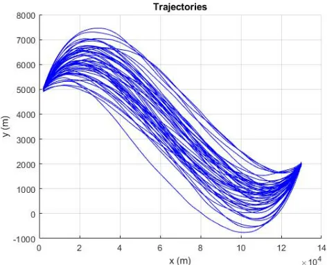
In Chapter 7, we propose the use ofCMLsequences for destination-directed trajectory mod-eling. Considering the main components of destination-directed trajectories, we demonstrate how naturally one would use the CML sequence for modeling such trajectories. This class of CM sequences provides a general framework for modeling destination-directed trajectories. The CML sequence models the main components of destination-directed trajectories and the only assumption in its definition is the Markov-like (i.e., conditionally Markov) property of its evo-lution law. We show how parameters of aCML model can be designed for destination-directed trajectory modeling. TheCMLsequence enjoys several desirable properties for trajectory mod-eling (for example in ATC). The GaussianCML sequence, its realization, its properties, and its dynamic model (theCML model) are studied for the purpose of trajectory modeling. Filtering and prediction formulations are derived based on the CML model. The behavior of the filter is studied. Trajectory predictors with and without destination information are compared based on their formulations and some simulations. Several simulations are presented to demonstrate the results.

1.2.8 Conventions and Notations

We give conventions used in multiple chapters of the dissertation.

We consider stochastic sequences defined over the interval [0, N], which is a general discrete-index interval. For convenience this discrete-discrete-index is called time. The following conventions are used:

[i, j],{i, i+ 1, . . . , j−1, j}, i < j

[xk]ji ,{xk, k∈[i, j]}

(22)

x,[x0₀, x0₁, . . . , x0_N]0 i, j, k1, k2, l1, l2 ∈[0, N]

σ([xk]j_i),σ-field generated by [xk]j_i

wherekin [xk]j_i is a dummy variable. [xk] is a stochastic sequence. [xk]j_i is not defined fori > j. Also,σ([xk]ji), fori > j, andσ([xk]cc\ {xc}) are defined as the trivialσ-field (i.e., including only the empty set and the whole set Ω). The symbols “0” and “\” are used for matrix transposition and set subtraction, respectively. In addition, 0 may denote a zero scalar, vector, or matrix, as is clear from the context. P{·}denotes probability and F(·|·) denotes a conditional comulative distribution function (CDF). Also, p(·) and p(·|·) are a probability density function (PDF) and a conditional PDF, respectively. R denotes the set of real numbers. N(µk, Ck) denotes the Gaussian distribution with mean µk and covariance Ck. Also, N(xk;µk, Ck) denotes the corresponding Gaussian density with (dummy) variable xk. Ci,j is a covariance function, and Ci , Ci,i. C is the covariance matrix of the whole sequence [xk] (C = Cov(x)). A Gaussian sequence [xk] is nonsingular if its covariance matrixC is nonsingular. The abbreviations ZMNG and NG are used for “zero-mean nonsingular Gaussian” and “nonsingular Gaussian”. For a matrix A, A_[_r₁_:_r₂_,c₁_:_c₂_] denotes its submatrix consisting of (block) rows r1 to r2 and (block)

columns c1 toc2 of A. For square matricesMk, we have

diag(M0, M1, . . . , MN),



   

M0 0 · · · 0

0 M1 · · · 0

..

. ... . .. ... 0 · · · 0 MN



   

The evolution of a sequence can be modeled by a forward or a backward model. The for-ward direction is the default. For forfor-ward direction/models, we drop the term “forfor-ward”, but for backward direction/models we make “backward” explicit. We have different dynamic models in-cluding a Markov model, a reciprocal model, a reciprocalCML/CMF model, and aCML/CMF model. For example, a Markov model has an initial condition and aCMLmodel has a boundary condition. For unification, we may call an initial condition a boundary condition. Sometime we need to refer to a dynamic model including its boundary condition, but sometimes we need to refer to a dynamic model without its boundary condition. The term “dynamic model” or “model” is used to refer to both these cases when the meaning is clear from the context. But to avoid confusion in some cases we use the term “evolution model” to emphasize that we mean a dynamic model without considering its initial/boundary condition. For example, a “Markov evolution model” means a Markov model without considering its initial condition. Also, a “CML evolution model” means aCML model without considering its boundary condition.

(23)

Chapter 2

Modeling and Characterizing Nonsingular Gaussian CM Sequences

In this chapter, we 1) provide useful and easy to apply results for application of CM sequences, e.g., for motion trajectory modeling with destination information, and 2) lay a foundation for studying an important special class of CM sequences, the reciprocal sequence, from the CM viewpoint.

2.1 Definitions and Preliminaries

To build a solid foundation, we start from definitions in the formal probability language. How-ever, all the main results are presented in a simple language ready for application. We assume the stochastic sequences are defined with respect to an underlying probability triple (Ω,A, P).

2.1.1 CM Definitions and Notations

A sequence [xk] is [k1, k2]-CMc, c∈ {k1, k2}, (i.e., CM over [k1, k2]) iff conditioned on the state

at timek1 (k2), the sequence is Markov over [k1+1, k2] ([k1, k2−1]). To build a solid foundation,

we need a formal definition of CM sequences (Definition 2.1.1 below). To provide results for application, however, later we present Corollary 2.1.5, which is equivalent to Definition 2.1.1.

Definition 2.1.1. [xk]is [k1, k2]-CMc, c∈ {k1, k2}, if for every j∈[k1, k2]

P{AB|xj, xc}=P{A|xj, xc}P{B|xj, xc} (2.1)

where A∈σ([xk]k2

j+1\ {xc}) and B ∈σ([xk]

j−1

k1 \ {xc}).

The interval [k1, k2] of a [k1, k2]-CMcsequence is called theCM interval of the sequence. By

Definition 2.1.1, the sequence is defined over the interval [0, N] but the CM interval is [k1, k2].

Remark 2.1.2. We use the following notation

[k1, k2]-CMc=

[k1, k2]-CMF if c=k1

[k1, k2]-CML if c=k2

where the subscript “F” or “L” is used because the conditioning is at the first or the last time of the CM interval.

Remark 2.1.3. When the CM interval of a sequence is the whole time interval, it is dropped: a [0, N]-CMc sequence is called CMc.

(24)

We define that every sequence with a length smaller than 3 (i.e., {x0, x1}, {x0}, and {}) is

Markov. Similarly, every sequence is [k1, k2]-CMc,|k2−k1|<3. So, CMLand CML∩[k1, N

]-CMF,k1∈[N −2, N] are the same.

Assuming [xk] is a [k1, k2]-CMc sequence, then [xk]k_k2₁ is a CMc sequence.

Different values ofk1,k2, andcdefine different classes of CM sequences. For example,CMF and [1, N]-CML are two classes. ByCMF ∩[1, N]-CMLwe mean a sequence being both CMF and [1, N]-CML. We use similar notations for intersections of other classes.

2.1.2 Preliminaries (for Gaussian CM Sequences)

In this subsection, some results are presented, to be used in proofs in later sections. The goal is to find simple necessary and sufficient conditions for Gaussian sequences to be CM.

Lemma 2.1.4. [xk]is [k1, k2]-CMc, c∈ {k1, k2}, iff for every Borel measurable function f,

E[f(xk)|[xi]j_k

1, xc] =E[f(xk)|xj, xc] (2.2)

for everyj, k∈[k1, k2], j < k, or equivalently,

E[f(xk)|[xi]kj2, xc] =E[f(xk)|xj, xc] (2.3)

for everyk, j ∈[k1, k2], k < j.

Proof. We prove (2.2) first. It can be seen that Definition 2.1.1 of the [k1, k2]-CMc sequence and (2.4) below are equivalent; that is, [xk] is [k1, k2]-CMc iff

P{A|[xi]j_k₁, xc}=P{A|xj, xc] (2.4)

for everyj∈[k1, k2−1], whereA∈σ([xk]k_j2₊₁\ {xc}) [85], [6]. Also, (2.4) holds iff

E[h([xi]k2

j+1\ {xc})|[xi]

j

k1, xc] =E[h([xi] k2

j+1\ {xc})|xj, xc] (2.5)

for everyj ∈[k1, k2−1] and every Borel measurable functionh. Clearly (2.2) follows from (2.5).

So, we need to show that if (2.2) holds, so does (2.5). We will do it by mathematical induction on j. For j=k2−1, (2.5) follows from (2.2). Fixl∈[k1, k2−2]. Assume that (2.5) holds for

j=l+ 1, that is,

E[g([xi]k_l₊₂2 \ {xc})|[xi]l_k+1₁ , xc] =E[g([xi]k_l₊₂2 \ {xc})|xl+1, xc] (2.6) for every Borel measurable functiong. Then, we prove that it holds forj=l,

E[h([xi]k_l₊₁2 \ {xc})|[xi]lk1, xc] =E

h

E[h([xi]k_l₊₁2 \ {xc})|[xi]lk1, xl+1, xc]

[xi]

l k1, xc

i

=E h

E[h([xi]k2

l+1\ {xc})|xl, xl+1, xc]

[xi]

l k1, xc

i

=EhE[h([xi]k_l₊₁2 \ {xc})|xl, xl+1, xc] xl, xc

i

=E[h([xi]k_l₊₁2 \ {xc})|xl, xc] (2.7) for every Borel measurable functionh. Note that the second equality follows from (2.6), and the third equality is due to (2.2) (note thatE[h([xi]k2

l+1\ {xc})|xl, xl+1, xc] is a function ofxl,xl+1,

and xc). By mathematical induction, (2.5) is concluded. (Note that the required integrability condition for nested expectations [86] holds.)

The following has been used in the third equality of (2.7). By Corollary 2.1.5 below, (2.8) below follows from (2.2)

F(ξl+1|[xi]lk1, xc) =F(ξl+1|xl, xc),∀ξl+1 ∈R

(25)

where F(·|·) is the conditional CDF of xl+1 and dis the dimension of xl+1. Then, (2.9) below

follows from (2.8):

F(ξl, ξl+1, ξc|[xi]lk1, xc) =F(ξl, ξl+1, ξc|xl, xc) (2.9)

where F(·|·) is the conditional CDF of xl,xl+1, andxc. On the other hand, letg1(xl, xl+1, xc)

= E[h([xi]kl+12 \ {xc})|xl, xl+1, xc]. By the definition of conditional expectation, g1 is a Borel

measurable function. Based on (2.9), it is concluded that (see the proof of Corollary 2.1.5 for more details)

E[g1(xl, xl+1, xc)|[xi]lk1, xc) =E[g1(xl, xl+1, xc)|xl, xc) (2.10)

which has been used in the third equality of (2.7). A similar fact has been used in the second equality of (2.7), too.

A proof of (2.3) is similar. To prove sufficiency, it suffices to show that (2.11) follows from (2.3) by mathematical induction. (Observe that forj=k1+ 1, (2.11) follows from (2.3). Then,

assume (2.11) holds for j=l−1 (fix l∈[k1+ 2, k2]) and prove it for j=l.)

E[h([xi]j_k−1

1 \ {xc})|[xi] k2

j , xc] =E[h([xi] j−1

k1 \ {xc})|xj, xc] (2.11)

Corollary 2.1.5. [xk]is [k1, k2]-CMc, c∈ {k1, k2}, iff its CDF satisfies

F(ξk|[xi]j_k₁, xc) =F(ξk|xj, xc),∀ξk∈Rd (2.12)

F(ξk|[xi]k2

j , xc) =F(ξk|xj, xc),∀ξk∈R

d _(2.13)

for everyk, j ∈[k1, k2], k < j, where dis the dimension of xk.

Proof. It is enough to show that (2.2) is equivalent to (2.12) and (2.3) is equivalent to (2.13). We briefly address the former and skip the latter, since they are similar.

Assume (2.2) holds. Then, let f(xk) = 1A(xk) (1A(xk) = 1 for xk ∈ A, and 1A(xk) = 0 for xk ∈/ A), where A = {x1_k ≤ξ_k1} × {x2_k ≤ ξ_k2} × · · · × {xd_k ≤ ξ_kd}, xk = [x1_k, x2_k, . . . , xd_k]0, and ξk= [ξk1, ξ2k, . . . , ξkd]

0_{. Then, the RHS (LHS) of (2.2) is equal to the RHS (LHS) of (2.12).}

Assume (2.12) holds. Then, P{B|[xi]j_k

1, xc} = P{B|xj, xc} for every B ∈ σ(xk) [87], and (2.2) is concluded.

Remark 2.1.6. Due to simplicity we recommend considering Corollary 2.1.5 as the definition of [k1, k2]-CMc sequences in application.

For Gaussian sequences, Lemma 2.1.4 is equivalent to the following.

Lemma 2.1.7. A Gaussian sequence [xk]is [k1, k2]-CMc, c∈ {k1, k2}, iff

E[xk|[xi]j_k₁, xc] =E[xk|xj, xc] (2.14)

E[xk|[xi]k2

j , xc] =E[xk|xj, xc] (2.15)

(26)

Proof. We prove (2.14). Proof of (2.15) is similar and is skipped. Necessity: By Lemma 2.1.4, for a [k1, k2]-CMc sequence [xk], (2.14) holds.

Sufficiency: Let [xk] be a Gaussian sequence for which (2.14) holds. The conditional covari-ance can be calculated as

Cov(xk|[xi]j_k₁, xc) =E h

xk−E[xk|[xi]j_k₁, xc]

·0 [xi]

j k1, xc

i

On the other hand, for conditional expectation we haveE[(xk−E[xk|[xi]j_k

1, xc])g([xi] j

k1, xc)] = 0 for every Borel measurable function g. Thus, xk−E[xk|[xi]jk1, xc] is orthogonal to (and due to Gaussianity independent of) [xi]j_k₁ and xc. Therefore, noting (2.14), we have

Cov(xk|[xi]jk1, xc) =E

h

xk−E[xk|xj, xc]

·0i

=Ehxk−E[xk|xj, xc]

·0 xj, xc

i

= Cov(xk|xj, xc) (2.16)

Due to Gaussianity, (2.14) and (2.16) lead to the equality of the corresponding conditional distributions. In other words, a Gaussian conditional distribution is completely determined by its conditional expectation [57]. Therefore, (2.2) holds and the sequence [xk] is [k1, k2]-CMc.

2.2 Dynamic Models of CMc Sequences

The CMc sequence is an important class of CM sequences. For example, a CML sequence can be used for motion trajectory modeling with destination information (Chapter 7). In addition, CML and CMF sequences play a very important role in the study of the reciprocal sequence from the CM viewpoint.

A dynamic model for the zero-mean nonsingular Gaussian (ZMNG) reciprocal sequence was presented in [18]. Inspired by [18], we first present a model for evolution of the ZMNG CMc sequence, called a CMc model. Then, we discuss a model of the nonsingular Gaussian (NG) CMcsequence. The following lemma demonstrates construction of aCMcmodel for the ZMNG CMcsequence.

Lemma 2.2.1. Let [xk] be a ZMNG CMc sequence with covariance function Cl1,l2. Then, its evolution obeys

xk=Gk,k−1xk−1+Gk,cxc+ek, k∈[1, N]\ {c} (2.17)

where [ek](Gk=Cov(ek)) is a zero-mean white NG sequence, and boundary condition1

x0=e0, xc=Gc,0x0+ec(forc=N) (2.18) or equivalently2

xc=ec, x0 =G0,cxc+e0 (for c=N) (2.19)

Proof. We prove the lemma in three steps: (i) model construction, (ii) boundary conditions and the whiteness of [ek], and (iii) nonsingularity of covariance matrices Gk, k∈[0, N].

(i) Model construction: Since [xk] is CMc, by Lemma 2.1.7 for everyk∈[1, N]\ {c}we have

E[xk|[xi]k0−1, xc] =E[xk|xk−1, xc] (2.20)

1_{Note that (2.18) means that for} _c₌_N _{we have} _x

0 =e0 and xN =GN,0x0+eN. Also, for c= 0 we have

x0=e0. It is similar for (2.19). 2

It should be clear thate0 andeN in (2.18) and in (2.19) are not necessarily the same. Just for simplicity we

(27)

Since [xk] is Gaussian, for c = 0 and k = 1 we have E[xk|xk−1, xc] = C1,0C₀−1x0. Let G1,0 , 1

2C1,0C

−1

0 . For other c and kvalues (i.e.,c= 0 and k∈[2, N], andc=N and k∈[1, N −1]),

E[xk|xk−1, xc] = [Ck,k−1 Ck,c]

Ck−1 Ck−1,c Cc,k−1 Cc

−1 xk−1

xc

Let [Gk,k−1 Gk,c] , [Ck,k−1 Ck,c]

−1

. So, for every k ∈ [1, N]\ {c} and

c∈ {0, N}, we have E[xk|xk−1, xc] =Gk,k−1xk−1+Gk,cxc. Defineek,k∈[1, N]\ {c}, as

ek=xk−E[xk|xk−1, xc] (2.21)

=xk−Gk,k−1xk−1−Gk,cxc

Then, forc= 0 and k= 1, G1,Cov(e1) =C1−C1,0 ·C0−1C10,0. For other cand k values,

Gk ,Cov(ek) =Ck−[Ck,k−1 Ck,c]

−1

[Ck,k−1 Ck,c]0

[ek][1,N]\{c} is a zero-mean white Gaussian sequence uncorrelated with x0 and xc. It can be verified as follows. By the definition of conditional expectation and based on (2.20) we have

E[(xk−E[xk|xk−1, xc])g([xj]0k−1, xc)] =E[(xk−E[xk|[xi]k

−1

0 , xc])g([xj]k

−1

0 , xc)] = 0 (2.22)

for every Borel measurable function g. Thus, by (2.21) and (2.22), ek is uncorrelated with [xi]k₀−1 and xc. Then, fork≥j,

E[eke0j] =E[ek(xj −Gj,j−1xj−1−Gj,cxc)0] =

Gk k=j

0 otherwise (2.23)

Likewise for j≥k. Therefore, E[eke0k] =Gk and E[eke0j] = 0, k6=j. So, [ek][1,N]\{c} is white.

(ii) Boundary conditions: For c = 0, we have G0 , C0. Let c = N and consider (2.18).

Since x0 and xN are jointly Gaussian, we have E[xN|x0] = GN,0x0, where GN,0 = CN,0C0−1.

Then, we define eN , xN − GN,0x0, where eN is a ZMNG vector with covariance GN =

CN−CN,0C0−1CN,0 0. Also, by the definition of conditional expectation,eN is uncorrelated with x0(i.e.,E[(xN−E[xN|x0])g(x0)] = 0 for every Borel measurable functiong). Also, for notational

unification e0,x0 with covariance G0,C0.

Similarly for c = N and (2.19), we have x0 = G0,N xN +e0, G0,N = C0,NC_N−1, and G0 =

C0−C0,NCN−1C00,N, wheree0 is a ZMNG vector with covarianceG0, uncorrelated withxN. Also, set eN ,xN with covarianceGN ,CN.

By (2.22), [ek][1,N]\{c} is uncorrelated withx0 and xc, and thus uncorrelated withe0 andec.

So, [ek] is white.

(iii) From (2.30) in the proof of Lemma 2.2.5 below, nonsingularity of the covariance matrices Gk,k∈[0, N], follows from nonsingularity of the covariance matrix of [xk].

Lemma 2.2.2. Forc=N, the boundary conditions(2.18)and(2.19)can be obtained from each other.

Proof. For clarity, denote (2.18) and (2.19) as

x0 =e10, xN =GN,0x0+e1N (2.24)

xN =eN, x0 =G0,NxN +e0 (2.25)

(28)

be easily seen that e0 and eN are uncorrelated with [ek]N1 −1, because e10, e1N, x0, and xN are uncorrelated with [ek]N1 −1. Also,

E[e0e0N] =E[(e10−G0,NxN)(e1N +GN,0x0)0]

=E[e1₀(e_N1 )0] +E[e1₀x0₀]G0_N,₀−G0,NE[xN(e1N)

0_]₋_G

0,NE[xNx00]G

0

N,0

=E[e1₀(e1₀)0]G0_N,₀−G0,NE[(GN,0e10+e1N)(e1N)0]−G0,NE[(GN,0e10+e1N)(e10)0]G0N,0

=G1₀G0_N,₀−G0,NGN1 −G0,NGN,0G10G0N,0

=C0(CN,0C0−1)

0₋_C

0,NCN−1(CN −CN,0C0−1C0,N)−C0,NCN−1CN,0C0−1C0,N = 0 which means e0 and eN are uncorrelated. Similarly, one can obtain (2.24) from (2.25).

So, for c = N, (2.18) and (2.19) have different forms, but are equivalent. Therefore, for brevity later we may refer to only one of them, although similar results hold for the other.

Remark 2.2.3. Boundary condition(2.19)emphasizes the role and importance ofxN in aCML model (i.e., the evolution law fromk= 0 to k=N−1 depends onxN).

It is important that a dynamic model gives a unique covariance function of the corresponding sequence [18]. As the following lemma shows, this is the case for model (2.17).

Lemma 2.2.4. Model (2.17) along with (2.18) or (2.19) for every parameter value admits a unique covariance function.

Proof. Let [xk] obey (2.17) along with (2.18) or (2.19) withc=N. That is,

Gx=e, e_,[e0₀, . . . , e0_N]0 (2.26) whereGwill be given below. Post-multiplying both sides byx0 and taking expectation, we have

GC=U, where C= Cov(x) and U = Cov(e, x).

To show the uniqueness of the covariance function, it suffices to show that G is nonsingular. Consider (2.18) for whichG is

        

I 0 0 · · · 0 0

−G1,0 I 0 · · · 0 −G1,N 0 −G2,1 I 0 · · · −G2,N

..

. ... ... ... ... ...

0 0 · · · −GN−1,N−2 I −GN−1,N

−GN,0 0 0 · · · 0 I

         (2.27)

The determinant of a partitioned matrix A=

A11 A12

A21 A22

is |A|=|A11| · |A22| ifA12 = 0 or

A21= 0 [88]. So, it can be seen that|G| 6= 0 for every choice of the parameters, as follows. Since

G_[1:1_,_2:_N_+1] = 0, we have |G|= |G_[2:_N₊₁_,_2:_N_+1]|. For a similar reason (i.e. G_[_N_+1:_N₊₁_,_2:_N_] = 0), we have |G_[2:_N₊₁_,_2:_N_+1]| =|G_[2:_N,_2:_N_]|, where it is clear that |G_[2:_N,_2:_N_]|= 1. Therefore, model (2.17)–(2.18) always admits a unique covariance function.

Since (2.18) and (2.19) are equivalent (Lemma 2.2.2), model (2.17) with (2.19) always admits a unique covariance function, too. It can be also verified based on the nonsingularity of G

corresponding to (2.19), which is

        

I 0 0 · · · 0 −G0,N

−G1,0 I 0 · · · 0 −G1,N 0 −G2,0 I 0 · · · −G2,N

..

. ... ... ... ... ...

0 0 · · · −GN−1,N−2 I −GN−1,N

0 0 0 · · · 0 I

(29)

Let [xk] obey (2.17)–(2.18) with c= 0. That is, Gx=e, e,[e00, . . . , e0N]

0_{, where}_G _is



       

I 0 0 · · · 0 0

−2G1,0 I 0 · · · 0 0

−G2,0 −G2,1 I 0 · · · 0

..

. ... ... ... ... ...

−GN−1,0 0 · · · −GN−1,N−2 I 0

−GN,0 0 0 · · · −GN,N−1 I



       

(2.29)

Since (2.29) is nonsingular, (2.17)–(2.18) always admits a unique covariance function.

Lemma 2.2.5. [xk]governed by(2.17)–(2.18)is always nonsingular (for every parameter value).

Proof. Let [xk] obey (2.17)–(2.18), where the covariance matrices Gk,k∈[0, N], are nonsingu-lar. Based on (2.26), we have Gx=e, where G is given by (2.27) for c =N and by (2.29) for c= 0. Then, the covariance matrix of [xk] can be obtained as

C=G−1_G₍_G0₎−1 _(2.30)

whereG= Cov(e) = diag(G0, . . . , GN) and by the proof of Lemma 2.2.4,Gis nonsingular. Since all Gk,k∈ [0, N], are nonsingular, Gis nonsingular. Therefore, by (2.30), [xk] is nonsingular.

By the previous lemmas, a model for the ZMNG CMc sequence was constructed and some related properties were studied. Now, we can present the main result for the CMc model as follows.

Theorem 2.2.6. A ZMNG sequence [xk] with covariance function Cl1,l2 is CMc iff it obeys (2.17) along with (2.18)or (2.19).

Proof. The necessity was proved as Lemma 2.2.1. So, we just need to prove the sufficiency. This amounts to proving that [xk] is (i) nonsingular and (ii) GaussianCMc. Lemma 2.2.5 has established (i). So, we just need to prove (ii).

Since [xk] is Gaussian, by Lemma 2.1.7, [xk] isCMcifE[xk|[xi]j₀, xc] =E[xk|xj, xc], for every j, k∈[0, N]\ {c}, j < k. From (2.17) we havexk =Gk,jxj+Gk,c|jxc+ek|j, where the matrices Gk,j and Gk,c|j can be obtained from parameters of (2.17), and ek|j is a linear combination of [el]kj+1. Since [ek] is white, [el]jk+1 (and soek|j) is uncorrelated with [xk]j0 andxc. Thus, we have

E[xk|[xi]j0, xc] =E[xk|xj, xc], meaning that [xk] isCMc.

Let z ∼ N(µz, Cz) and y ∼ N(µy, Cy) be jointly Gaussian random vectors with

cross-covariance Cz,y. Also, let ˇz and ˇy be zero-mean parts of z and y, respectively. We have E[z|y] = µz+Cz,yC_y+(y−µy), where ‘+’ denotes the Moore-Penrose inverse. On the other hand, E[ˇz|yˇ] = Cz,yC_y+(ˇy). So, E[z|y]−µz = E[ˇz|yˇ]. Then, by Lemma 2.1.7, a Gaussian sequence isCMc iff its zero-mean part isCMc. Therefore, a Gaussian sequence [xk] with mean function µk, k∈ [0, N], is CMc iff its zero-mean part [xk−µk] obeys (2.17)–(2.18). Thus, we only present models of zero-mean CM sequences.

Backward Markov/hybrid models have been developed and used, e.g., for smoothing [65]– [71], [89]. The evolution of theCMc sequence can also be modeled by a backwardCMcmodel. A backwardCMcmodel may provide more insight and tools regarding theCMcsequence. Also, it is useful for smoothing. The next proposition presents a backward CMc model.

Proposition 2.2.7. A ZMNG [xk] isCMc iff