Predicting Voltage Abnormality Using Power System Dynamics

(1)

University of New Orleans University of New Orleans

ScholarWorks@UNO

University of New Orleans Theses and

Dissertations Dissertations and Theses

Fall 12-20-2013

Predicting Voltage Abnormality Using Power System Dynamics

Nagendrakumar Beeravolu [email protected]

Follow this and additional works at: https://scholarworks.uno.edu/td

Part of the Power and Energy Commons

Recommended Citation Recommended Citation

Beeravolu, Nagendrakumar, "Predicting Voltage Abnormality Using Power System Dynamics" (2013). University of New Orleans Theses and Dissertations. 1722.

https://scholarworks.uno.edu/td/1722

This Dissertation is protected by copyright and/or related rights. It has been brought to you by ScholarWorks@UNO with permission from the rights-holder(s). You are free to use this Dissertation in any way that is permitted by the copyright and related rights legislation that applies to your use. For other uses you need to obtain permission from the rights-holder(s) directly, unless additional rights are indicated by a Creative Commons license in the record and/ or on the work itself.

(2)

Predicting Voltage Abnormality Using

Power System Dynamics

A Dissertation

Submitted to the Graduate Faculty of the University of New Orleans in partial fulfillment of the requirements for the degree of

Doctor of Philosophy In

Engineering and Applied Sciences Electrical Engineering

By

Nagendrakumar Beeravolu

(3)

Acknowledgements

This dissertation would not have been possible without the guidance and the help of

several individuals who in one way or another contributed and extended their valuable assistance

in the preparation and completion of this study.

First I wish to express my utmost gratitude to my advisor Prof. Dr. Parviz Rastgoufard

who was abundantly helpful and offered invaluable assistance, support and guidance to finish

this dissertation. My association with him for over six years was a rewarding experience. I am

really thankful to the members of the supervisory committee Dr. Ittiphong Leevongwat, Dr. Edit

Bourgeois, Dr. Bhaskar Kura, and Dr. George Ioup for their great support throughout my masters

to finish this study. I would like to thank Entergy-UNO Power and Research Laboratory for

providing appropriate tools to finish this task.

Last, I would like to acknowledge and thank my parents, my sister and all of my friends

(4)

List of Figures

Figure 1.1: Classification of Power System Stability ... 3

Figure 2.1: A two-bus test system... 18

Figure 2.2: P-V Curve ... 20

Figure 2.3: Operational time frame of equipment in power systems [2] ... 26

Figure 2.4: One line diagram of a simple four bus power system [14] ... 27

Figure 2.5: Circuit equivalent representation of four bus power system ... 27

Figure 2.6: Time-scale decomposition [14] ... 33

Figure 3.1: Methodology flowchart for voltage stability prediction... 38

Figure 3.2: Flow chart for Phase-I: Step-A ... 40

Figure 3.3: Flow chart for Phase-I: Step-B ... 41

Figure 3.4: Flow chart for Phase-I: Step-C ... 42

Figure 3.5: Flow chart for Phase-II: Step-A ... 43

Figure 3.6: Flow Chart of Pattern Recognition Model [40]... 45

Figure 3.7: Classification Trees - After a successive sample partitions, a classification decision is made at the terminal nodes ... 49

Figure 4.1 IEEE 39 Bus System [50] ... 53

Figure 5.1 Bus 7 Voltage for Stable Case 40 ... 68

Figure 5.2 Zoomed in Figure 5.1 ... 69

Figure 5.3 Bus 7 Voltage for Unstable Case 39... 70

Figure 5.4 Zoomed in Figure 5.3 ... 71

Figure 5.5 Feature 1, Feature 2, and Feature 3 ... 72

Figure 5.6 Relative Cost for the Classification Tree Topology ... 75

Figure 5.7 CART Tree Grooved for the Training Set ... 76

Figure 5.8 CART Tree for the Test Set ... 77

(7)

List of Tables

Table 4.1 Transmission Line Data ... 54

Table 4.2 Transformers Data ... 56

Table 4.3 Generators Initial Load Flow Details ... 57

Table 4.4 Generator Details ... 57

Table 4.5 Generators Excitation System Details ... 58

Table 4.6 Load Data ... 59

Table 5.1 Applied Contingencies for the IEEE39 Bus Test System... 61

Table 5.2 Features Extracted From System Parameters ... 73

Table 5.3 Accuracy of CART on Training Sets ... 77

Table 5.4 Accuracy of CART on Test Sets... 78

Table 5.5 Accuracy of RLSC Pattern Recognition Method for Different λ Values ... 80

Table 5.6 Prominent Features from RLSC ... 80

Table 5.7 Accuracy of RLSC on Training Sets ... 81

Table 5.8 Accuracy of RLSC on Test Sets ... 81

Table 5.9 Accuracy of CART Pattern Recognition Method ... 82

(8)

Abstract

The purpose of this dissertation is to analyze dynamic behavior of a stressed power

system and to correlate the dynamic responses to a near future system voltage abnormality. It is

postulated that the dynamic response of a stressed power system in a short period of time-in

seconds-contains sufficient information that will allow prediction of voltage abnormality in

future time-in minutes. The PSSE dynamics simulator is used to study the dynamics of the IEEE

39 Bus equivalent test system. To correlate dynamic behavior to system voltage abnormality, this

research utilizes two different pattern recognition methods one being algorithmic method known

as Regularized Least Square Classification (RLSC) pattern recognition and the other being a

statistical method known as Classification and Regression Tree (CART). Dynamics of a stressed

test system is captured by introducing numerous contingencies, by driving the system to the

point of abnormal operation, and by identifying those simulated contingencies that cause system

voltage abnormality.

Normal and abnormal voltage cases are simulated using the PSSE dynamics tool. The

results of simulation from PSSE dynamics will be divided into two sets of training and testing set

data. Each of the two sets of data includes both normal and abnormal voltage cases that are used

for development and validation of a discriminator. This research uses stressed system simulation

results to train two RLSC and CART pattern recognition models using the training set obtained

from the dynamic simulation data. After the training phase, the trained pattern recognition

algorithm will be validated using the remainder of data obtained from simulation of the stressed

(9)

Each of the algorithmic or statistical pattern recognition methods have their advantages

and disadvantages and it is the intention of this dissertation to use them only to find correlations

between the dynamic behavior of a stressed system in response to severe contingencies and the

outcome of the system behavior in a few minutes into the future.

Key Words: Pattern recognition; Power system dynamic response; Blackouts; Voltage stability;

(10)

Chapter 1

1 Introduction

1.1 Power System Stability

Security of power systems operation is gaining ever increasing importance as the system

operates closer to its thermal and stability limits. Power system stability can be defined as:

– Is the ability of an electric power system, for a given initial operating condition,

to regain a state of operating equilibrium after being subjected to a physical

disturbance, with most system variables bounded so that practically the entire

system remains intact.

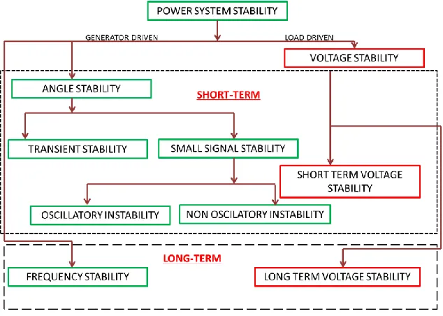
Power system stability, the most important index in power system operation- may be

categorized under two general classes relating to the voltage stability and to the angle stability

driven by different forces in the system. Voltage stability is principally load driven and focuses

on determining the proximity of bus voltage magnitudes to pre-determined and acceptable

voltage magnitudes. Angle stability is principally generator driven focuses on the investigation

of voltage angles as the balance between supply and demand changes due to occurrence of faults

or disturbances in the system and this affects voltage magnitudes as well. Voltage stability is a

slowly varying phenomena in seconds or minutes while angle stability is relatively faster in milli

seconds and deals with systems dynamics described mathematically by differential equations of

(11)

Power system stability can be classified in to the two different categories of voltage and

angle stability on the basis of [1]

 The physical nature of resulting mode of instability

 The size of the disturbance

 The devices, process and time span

 The most appropriate method of calculation and prediction of stability

Classification of power system stability on the basis of the criteria mentioned above is

presented in Figure 1.1. Since the classification is based on a number of diverse conditions, it is

difficult to select clearly distinct categories and to provide definitions that are rigorous and yet

convenient for practical use. Classification of power system stability is an effective and

convenient means to deal with the complexities of the problem, but one has to keep in mind that

the overall system stability is not affected and solutions to stability problems of one category

should not be at the expense of another.

This research will concentrate on voltage stability issues. The purpose of this dissertation

is to analyze dynamic behavior of a stressed power system and to correlate the dynamic

responses to a near future system voltage abnormality. The main goal of this dissertation is to

analyze dynamic behavior of a stressed power system and to correlate the dynamic responses to a

near future system voltage abnormality in order to provide the operators a lead time for remedial

(12)

Figure 1.1: Classification of Power System Stability

As this section has provided a basic idea of power system stability and the classification

of the stabilities in power systems, the next sections will cover the basics of voltage stability and

a review of the voltage stability analysis methods relevant to the main objective of this

dissertation.

1.2 A Review of Voltage Stability

Voltage stability can be defined as:

– A power system at any given state and subjected to a given disturbance is voltage

stable if the voltage near load buses approach post-disturbance equilibrium

values. Where the disturbed state is within the region of attraction of the stable

(13)

Voltage instability problems are more frequent on heavily stressed systems. After a system

disturbance, the consequence of voltage collapse may be influenced by a variety of factors such

as the strength of the transmission network, generator reactive power and voltage control limits,

load characteristics, characteristics of reactive compensation devices, and action of voltage

control device such as tap changing transformers.

A possible outcome of voltage instability is the loss of load or load shedding in an area

where the voltage is more degraded compared to the voltage in other areas of the system. The

main factor contributing to voltage instability in an area is an increase in voltage drop when

resulting from active and reactive power flow through the transmission line compared to initial

conditions. There is another possibility that an increase in rotor angles of generators will also

cause greater system voltage drop and result in voltage instability.

Voltage instability or voltage collapse in a power system is normally perceived as slowly

varying phenomena and it could be caused by variety of system dynamics. The mechanism

leading to voltage collapse normally starts as the voltage decreases in an area due to the increase

in load demand. The system steady state conditions change slowly initiating the voltage

stabilizing elements such as load tap changers, voltage regulators, and static and dynamic

compensators to respond, and correct the system changes. If these elements while stabilizing the

system exceed their operating limits, they will be removed from system operation. This may

prevent correction and system will degrade instead to a more severe operating condition, closer

to the point of voltage collapse, and eventually to operating conditions that are uncontrollable.

Because of interaction of these components and due to different dynamic time responses of these

(14)

to variation in time responses, appropriate mathematical models that capture dynamics in almost

real-time to steady state models may be required to predict proximity and occurrence of voltage

collapse in real-size power systems. The main reason for voltage collapse is when transmission

lines are operating very close to their thermal limits and then are forced to transmit more power

or when the power system has insufficient reactive power for transmission to an area with

increasing load requirements.

In large scale systems, voltage collapse includes voltage magnitude and angle under

heavy loading conditions. In some situations, it is hard to decouple the angle and magnitude

instability from each other.

Two types of system analysis are possible; static system and dynamic system analysis [1].

Each approach has its appropriate use for specific system conditions and each bears its own

advantages and disadvantages which will be addressed in this research. The design and analysis

of accurate methods to evaluate the voltage stability of a power system and to predict incipient

voltage instabilities are therefore of special interest in the field of power systems. Dynamic

analyses provide the most accurate indication of the time response of the system and are useful

for predicting fast occurring voltage collapses in the system but these will not provide much

information about sensitivity or degree of stability. On the other hand static analyses that are

based on performing system-wide sensitivity will provide the information necessary for

concluding degree of instability. Static analyses involve computation of algebraic equations

rather than the solution of differential equations, and hence, are much faster to compute

(15)

embedded in the energy content of the system only a few seconds after occurrence of a system

disturbance and long before the ultimate result of system voltage collapse.

This section has provided a brief introduction to voltage stability of a power system

including static and dynamic analysis of voltage stability, along with their advantages and

disadvantages. The upcoming sections of this chapter will provide a historical review of both of

the voltage stability analysis methods and will also outline our approach to using these models

for the prediction of patterns that may be detectible a few seconds after disturbances have

occurred.

1.3 Review of Static Analysis Methods of Voltage Stability

There is several research publications ranging from papers to books related to the static

analysis of voltage stability. Most of these publications document approaches that are based on

using the system’s Jacobian matrix and identification of singularities. The singularities of the

Jacobian matrix provide a guide to the point of system voltage collapse.

Static approaches capture snapshots of system conditions at various time frames and can

determine the overall stability of the system or proximity and margin to becoming unstable at

that particular time frame [1]. A variety of tools like multiple load flow solutions [3], load flow

feasibility [4], optimal power flow [5], steady state stability [6], modal analysis [2] [7] [8] [9]

[10] [11], the P-V curve, Q-V curve, Eigen value, singular value of Jacobian matrix [12] [13] ,

(16)

[1] [14] [15] [16] [17] [18] [19]. This section will only provide the methodology of each of these

static analysis methods. Chapter 3 of this dissertation report will elaborate on these methods.

In the past, all the utilities depended on conventional power flow programs for static

analysis and the voltage stability by computing P-V and V-Q curves at different buses in the

system while the load at these buses are increased. This method of static analysis is a time

consuming process because it has to undergo a large number of power flow solutions involving

several studies for each bus in the system. Also, the resulting P-V and V-Q curves will not

provide much information about the cause of instability since they are mainly concentrated on

individual buses in the power system network. There are some approaches such as V-Q

sensitivity modal analysis which provide more information regarding voltage stability [1].

V-Q sensitivity analysis which is used in modal analysis, is a good measure for the

sensitivity of a system [1]. This will use the same conventional power flow model and system

Jacobian matrix. Generally system voltage stability is affected by P and Q. For V-Q sensitivity

analysis, P is kept constant and the voltage stability is determined by considering incremental

relationship between Q and V. When P is kept constant the Jacobian matrix transforms to a

reduced Jacobian matrix. The inverse of this matrix becomes the reduced V-Q Jacobian matrix

where the ith diagonal element of the matrix is the V-Qsensitivity of the ith bus. A positive V-Q

sensitivity represents a stable operation. The smaller value of sensitivity implies a more stable

system so as the sensitivity value increases stability decreases. A negative value for V-Q

(17)

system. The smallest Eigen value is defined as the voltage stability margin and the singularity of

the Jacobian matrix, reflected by λmin=0, serves as the voltage instability indicator.

G.K. Morison, B. Gao, P. Kundar proposed a method referred to as V-Q modal analysis

[11] . This method is based on using the reduced Jacobian matrix formed in V-Q sensitivity

analysis to provide proximity of the system to voltage instability as well as the main contributing

factor for it. In this method, a smaller number of Eigen values are calculated from the reduced

Jacobian matrix which maintains the Q-V relationship of the network and also includes the

characteristics of generators, loads, reactive power compensating devices, and HVDC converters.

The Eigen values of reduced Jacobian matrix will identify different modes of the system which

will lead to voltage instability. The magnitude of the Eigen value provides a relative measure of

proximity to voltage instability. If the magnitude of modal Eigen value is equal to zero, then the

corresponding modal voltage collapses. Left and right Eigen vectors of critical modes will

provide the information concerning the mechanism for the voltage collapse by identifying the

elements that participate in the ultimate voltage collapse in the system. For this purpose, they

propose a concept called bus participation factor. Branches with large participation factors to the

critical mode will consume more reactive power for incremental change in reactive power and

will lead to the voltage instability.

S. Chandrabhan and G. Marcus have developed a PC-based MATLAB prototype

application [22] to analyze the voltage stability of a power network using the same modal

analysis proposed in [11] and some additional techniques like power flow analysis, V-P/V-Q

(18)

Modal analysis has some disadvantages [23] in requiring the Jacobian matrix to be a

square matrix, suitable for analyzing only PQ bus reactive power control where the active power

is considered as zero, and assumes constant voltages by not considering generator AVR at PV

buses.

C. Li-jun and E. Istavan [23] present their work by considering static voltage stability

analysis by the use of a singular value approach for both active and reactive power control. They

applied feasible controls as input signals and the voltage magnitude of critical buses as output

signals and developed a MIMO (multi input and multi output) transfer function of multi-machine

system and singular value decomposition (SVD) to identify the maximum and minimum singular

values of the transfer function matrix . The authors propose to monitor the maximum input and

output vectors and to relate the change to the input that has the largest influence on the

corresponding output and the buses where the voltage magnitude is critical.

Static analysis for voltage stability methods are easier to implement compared to dynamic

analysis methods because the modeling of loads and generators is relatively simple and requires

less computing time in the simulation. However these methods are not as accurate because of the

simplistic models.

This section has provided a review on static voltage stability analysis by introducing the

work performed by different researchers around the globe and provides a brief introduction to the

use of static voltage stability analysis methods. A review of dynamic stability analysis and a

(19)

1.4 Review of Dynamic Analysis Methods of Voltage Stability

A power system is typical a large dynamic system and its dynamic behavior has great

influence on the voltage stability. There are several ongoing research efforts related to the study

of dynamic voltage stability of power system to prevent the voltage collapse in the power system

subsequent blackouts.

In the dynamical analysis, voltage stability can be classified into short term, midterm and

long term dynamics based on the time scale of operation. By the name itself, short term

dynamics correspond to fast acting devices like generators and induction motors. Midterm and

long term dynamics correspond to slow acting devices like transformer load tap changers,

generator excitation limiters and generator automatic voltage regulators [2].

G. K. Morison, B. Gao, P. Kundar in [16] have shown how voltage instability can occur

and the situations in which the modeling of loads, load tap changers and generator maximum

excitation limiters will impact the system voltage stability. Reference [24] [25] investigated the

dynamic nature of voltage instability considering dynamic load modeling effect on the accuracy

of voltage stability analysis. To study dynamic voltage stability of a system, one needs to

consider the dynamic model for all the elements in the power system [26] and capture all the

dynamics of different elements in the system to find out the exact reason for voltage collapse. In

reference [27] voltage instability is associated with tap-changing transformer dynamics by

defining the voltage stability region in terms of allowable transformer settings. In reference [28]

the methods have employed a nonlinear dynamic model of OLTC, impedance loads and

decoupled reactive power voltage relations to reconstruct the voltage collapse phenomenon and

(20)

dynamic phenomenon of voltage collapse by dynamic simulations using induction motor models,

the paper explains how voltage collapse starts locally at the weakest node and eventually spreads

out to the other weak nodes.

K. Sun, S. Likathe, V. Vittal, V. S. Kolluri, S. Mandal [30] have proposed an online

dynamic security assessment scheme for large scale power systems using Phasor Measurement

Units (PMU) data and Decision Trees (DTs). This scheme will provide the dynamic security of

the power system from the available PMU real-time measurements and the DTs predictors

including fault type and location, bus voltage angles, MW transfers across lines or interfaces, and

generator output.

Cat S. M. Wong, P. Rastgoufard, and D. Mader in reference [31] used real time

simulation computing facilities to determine and detect signs and patterns of power system

dynamic behaviors to predict voltage stability.

system and to correlate the dynamic responses to the future system voltage abnormality. The

software package PSSE Dynamics simulator is used to study the dynamics of the IEEE 39 Bus

equivalent test system. To correlate dynamic behavior to system voltage abnormality, this

dissertation utilizes pattern recognition methods including algorithmic Regularized Least Square

Classification (RLSC) method and the statistical Classification and Regression Tree (CART)

method.

(21)

blackouts reported during the past and the reason behind the system voltage collapse will be

discussed.

1.5 Historical Review of Major Blackouts

There are several major power system blackouts that have occurred in last half century.

All the published reports on blackouts stated that even though each system was designed for N-1

contingencies, it was still not enough to secure stable system operations. An IEEE task force

report on “Blackout experiences and Lessons, Best Practices for System Dynamic Performance,

and the Role of New Technologies” [32] has reported on the major blackouts that have occurred

around the globe with the reasons behind the blackouts, and offered the best practices needed to

improve the dynamic performance of the system to avoid blackouts. The following are

summaries of some of the major blackout events that were reported.

The first major blackout reported was on November 9th 1965 in the United States

northeast area [33] [34]. Because of heavy loading conditions one of the five transmission lines

was tripped by a backup relay low load level settings. This resulted in tripping the remaining

four transmission lines causing 1700MW of load to be diverted to other lines there by over

loading them which resulted in voltage collapse. This blackout effected 30 million people and

New York City was in darkness for 13 hours. A special issue [35] published in 2005 talks about

changes made in power technology and policy after forty years from blackout occurred in 1965.

The next major blackout occurred on July 13th 1977 in the US [33] because of collapse in

the Con Edison System. A thunderstorm lightning strike hit two transmission lines and a

(22)

overloaded all the remaining transmission lines for 35 minutes causing them to trip. After 6

minutes the whole system was out of operation. This blackout left 8 million people in darkness

including New York City and took 5 to 25 hours to restore the system.

A decade later on July 23rd 1987 a major blackout occurred in Tokyo, Japan [33]. This

blackout occurred because of high peak demand due to extreme hot weather conditions. The

increased demand gradually reduced the voltage of the 500kV system to 460kV in five minutes.

The constant power characteristic loads such as air conditioning systems gradually reduced the

voltage and caused dynamic voltage collapse. The Tokyo blackout affected 2.8 million

customers with 3.8GW of load lost. The whole system was recovered relatively fast in 90

minutes after the voltage collapse.

The blackout on July 2nd 1996 in the Western North American power system [33] was

due to a short circuit of a 1300km series compensated 345kV transmission line caused by

flashover to a tree. This blackout affected 2 million people with 11,850MW of load loss.

The US-Canadian Blackout on August 14th 2003 [33] [36] was initiated by a 345kV

transmission line tripping due to a tree contact. Another line subsequently over loaded, sagged

and touched a tree after the first line was disconnected. At the same time, the supervisory control

and data acquisition (SCADA) system designed to warn operators was not functioning properly.

Several transmission lines reversed their power flow eventually causing a cascading blackout of

entire region. During this voltage collapse, 400 transmission lines and 531 generating units at

(23)

The European blackout occurred on November 4th 2006 [37] in the UCTE (Union for the

Coordination of the Transmission of Electricity) interconnected power grid which coordinates 34

transmission system operators in 23 European countries. This blackout started with a 380kV

transmission line tripping. This blackout affected 15 million people in Europe with 14.5 GW of

load interrupted in more than 10 countries.

The Arizona-Southern California outage occurred on September 8th 2011 [38] in United

States of America. An 11-minute system disturbance in the Pacific Southwest lead to cascading

outages and left approximately 2.7 million customers without power.

This section has reviewed the past major blackouts reported around the world. The next

section of this chapter will concentrate on the main purpose of this dissertation and explain the

methodology used in predicting voltage collapse.

1.6 Scope

This research continues the previous research completed at Tulane University by S. M.

Wong and P. Rastgoufard on “Unification of Angle and Magnitude Stability to Investigate

Voltage Stability of Large-Scale Power System” [31] [39] [40] [41], and at the University of

New Orleans by N Beeravolu and P. Rastgoufard on “Pattern Recognition of Power Systems

Voltage Stability Using Real Time Simulations” [42].

system and to correlate the dynamic responses to the future system voltage abnormality. It is

postulated that the dynamic response of a stressed power system in a short period of time-in

(24)

future time-in minutes [40] [42]. The PSSE Dynamics simulator software package was used to

study the dynamics of the IEEE 39 Bus equivalent test system. To correlate dynamic behavior to

system voltage abnormality, this research utilizes two pattern recognition methods including the

algorithmic Regularized Least Square Classification (RLSC) method and the statistical

Classification and Regression Tree (CART) method.

Normal and abnormal voltage cases are simulated using the PSSE Dynamics tool and the

results of the simulation from PSSE Dynamics will be divided into two sets of training and

testing data. Each of the two sets of data includes both normal and abnormal voltage cases that

are used for development and validation of a discriminator. This research uses stressed system

simulation results to train the RLSC and CART pattern recognition models using the training set

obtained from the dynamic simulation data. After the training phase, the trained pattern

recognition algorithm will be validated using the remainder of data obtained from simulation of

the stressed system. This process will determine the prominent features and parameters in the

process of classification of normal and abnormal voltage cases from dynamic simulation data.

The reminder of this dissertation discusses traditional methods for determining voltage

stability in Chapter 2, dissertation objectives and outline of methodology in Chapter 3, modeling

of the test system in Chapter 4, with results and voltage stability prediction analysis on the test

system in Chapter 5, Chapter 6 concludes with the summary of this dissertation and discusses

future work concerning the application of the proposed method.

(25)

Chapter 2

2 Methods of Voltage Stability Analysis

Chapter 1 of this dissertation has already provided some idea about the voltage stability

phenomenon. Voltage stability mainly deals with loads and voltage magnitudes. This chapter

discusses about traditional methods to determine the voltage stability.

As mentioned in Chapter 1, two types of system analysis are possible for voltage stability

studies; static system analysis and dynamic system analysis. Each approach may be used as

appropriate for specific system conditions. Each bears its own advantages and disadvantages

which we shall addressed in this research. Design and analysis of accurate methods to evaluate

the voltage stability of a power system and predicting incipient voltage instabilities are therefore

of special interest in the field of power systems. Dynamic analyses provide the most accurate

indication of the time response of the system and are useful for predicting fast occurring voltage

collapses in the system, however these studies will not provide much information about

sensitivity or degree of stability. On the other hand, static analyses that are based on performing

system-wide sensitivity studies will provide the information necessary for determining the

degree of instability for a system. Static analysis involves the computation of algebraic equations

rather than the solution of differential equations. Consequently it is much faster compared to

dynamic analysis for both on-line and off-line studies. That said, static analysis cannot

investigate the dynamic reasons for voltage instability that may be embedded in the energy

content of the system only a few seconds after occurrence of a system disturbance and long

(26)

in using static and dynamic system models for the prediction of patterns that may be detectible a

few seconds after disturbances to predict system voltage instabilities.

2.1 Static Voltage Stability Analysis methods

Static analysis for voltage stability captures snapshots of system conditions with various

time frames along the time-domain trajectory. The time derivatives of all the state variables are

assumed to be zero, so that the overall system equations are reduced to purely algebraic

equations. This dissertation will cover some of the traditional static voltage stability analyses in

the following sub-sections.

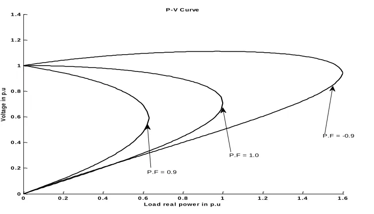
2.1.1 P-V Curve Analysis

P-V curve analysis is used to determine voltage stability of a radial system and also a large

meshed network. For this analysis P, i.e. power at a particular area, is increased in steps and the

resulting voltage V is observed at some critical load buses. Curves for those particular buses will

be plotted to determine the voltage stability of a system by a static analysis approach. The main

disadvantage of this method is that the power flow solution will diverge at the nose or maximum

power capability of the curve and the generation capability needs to be rescheduled as the load

increases.

To explain the P-V curve analysis let us assume a simple circuit which has a single

generator, single transmission line and a load. This circuit consists of two buses. The one line

(27)

P-V curves are useful in deriving how much load shedding should be done to establish

pre-fault network conditions even with the maximum increase of reactive power supply from

various automatic switching of capacitors or condensers.

Generator

R+JX

P

L

+

jQ

L

VS<δ1 VR<δ2

Load

Figure 2.1: A two-bus test system

Here the complex load assumed is SL =PL + jQL, where PL and QL real and reactive power

loads respectively. VR is the receiving end voltage and VS is the sending end voltage. R and X are

the respective resistance and reactance of the transmission line. CosΦ is the load power factor.

The complex load power can be written as Equation (2.1).

| | | || |( ) | || | _(2.1)

Let us consider . Equation (2.1) can be written as Equation (2.2).

( ) ( ) (2.2)

From equation (2.1), PL and QL can be written as Equation (2.3) and Equation (2.4).

| || | (2.3)

(28)

The network equations for the circuit considered for the case where resistance of

transmission line assumed as zero are given in Equation (2.5).

| || |

(2.5)

| | | || | (2.6)

Where - is the bus voltages angle difference.

| || |

| | (2.7)

Applying trigonometric identities on Equations (2.6) and (2.7) will produce Equation (2.8).

[ | | ] | | | | (2.8)

Solving Equation (2.8) for VR will give Equation (2.9).

| | | | [| | ( | | )] (2.9)

The Equation (2.9) can give P-V curve when the values of VS , β, and X are fixed. As P real

power load changes, two voltage solutions will result at each loading case. At P=Pmax, the

voltage solutions will be of the same value and this voltage is called the critical voltage. If P is

increased beyond Pmax, then the solution will become unsolvable indicating voltage collapse.

(29)

Figure 2.2: P-V Curve

2.1.2 V-Q Curve Analysis

V-Q curves plot voltage at a test or critical bus versus reactive power on the same bus.

V-Q curves will provide good insight in to system reactive power capabilities under both normal

and contingency conditions. The V-Q curves have many advantages. V-Q curves will show

reactive power margin at a test bus. Reactive power compensation will provide security to

voltage stability problems. This is determined by plotting reactive power compensations onto the

V-Q curves. The slope of the V-Q curve will indicate stiffness of the test bus. It should be noted

however that this method artificially stresses a single bus and should be confirmed by more

realistic methods before reaching a conclusion.

2.1.3 V-Q Sensitivity Analysis

The V-Q sensitivity analysis will provide information regarding the sensitivity of a bus

voltage with respect to the reactive power consumption. This analysis can provide system wide

0 0 .2 0 .4 0 .6 0 .8 1 1 .2 1 .4 1 .6

0 0 .2 0 .4 0 .6 0 .8 1 1 .2 1 .4 V o lta g e i n p .u

Loa d re a l powe r in p.u P - V C urve

P.F = 0.9

P.F = 1.0

(30)

voltage stability related information and can also identify areas that have potential problems. The

linearized steady state power systems equations can be expressed as Equation (2.10).

[ _{] [}

] [

] (2.10)

Where ΔP= vector of incremental change in bus real powers

ΔQ= vector of incremental change in bus reactive power injections

ΔV= vector of incremental change in bus voltage magnitude

Δθ= vector of incremental change in bus voltage angle

Here the elements of the Jacobian matrix J will give the sensitivity between power flow

(Real power P, Reactive power Q) and voltage (Bus Voltage Magnitude V and Angle )

changes.

The general structure of the system model for voltage stability analysis is similar to that

of transient stability analysis. The overall system equations, comprising a set of first-order

differential equations can be mathematically expressed as Equation (2.11).

̇ ( ) (2.11)

In Equation (2.11) X and V represent the state vector and bus voltage vector respectively.

Rewriting the linear relationship between power and voltage for each device when ̇=0

(31)

[ ] [

] [

] (2.12)

Here “d” stands for device.

All the above elements are for a particular device. A11, A12, A21 and A22 matrices will

represent system Jacobian elements.

V-Q sensitivity analysis is done by keeping the real power P constant and evaluating

voltage stability by considering the incremental relationship between Q and V. when ΔP=0 we

can derive Equation (2.13) from equation (2.10)

(2.13)

Where

[ ] (2.14)

JR is called as reduced Jacobian matrix of the system Equation 2.13 can also be written as

equation (2.15)

_(2.15)

Where JR-1 is the inverse of the reduced V-Q Jacobian and its ‘ith ’ diagonal element will provide

V-Q sensitivity at bus ‘I’.

As previously mentioned, V-Q sensitivity at a bus is the slope of Q-V curve at given

operating conditions. A positive V-Q sensitivity indicates a stable condition and negative

(32)

magnitudes of the sensitivities for different system conditions do not provide a direct measure of

the relative degree of stability.

2.1.4 Q-V Modal Analysis

Eigen values and Eigen vectors of reduced Jacobian matrix JR will be useful in describing

voltage stability characteristics.

Let us consider (2.16)

Where R= right Eigen vector matrix of JR

L= left Eigen vector matrix of JR

Λ=Diagonal Eigen value matrix of JR

Using modal transformation Equation (2.16) can be written as Equation (2.17).

_(2.17)

Substituting Equation (2.17) in to Equation (2.13) will give Equation (2.18)

_(2.18)

∑ (2.19)

Here ‘ri’ is the ‘ith’ column right Eigen vector and ‘li’ is the ‘ith’ row left Eigen vector.

(33)

_(2.20)

Substituting Equation (2.20) in Equation (2.10), we obtain Equation (2.21).

_(2.21)

_(2.22)

Where is vector of modal voltage analysis and is vector of modal reactive

power variations.

From Equation (2.22), we can write Equation (2.23).

(2.23)

And Λ-1 is diagonal matrix. Details of development of Equation (2.13) to (2.22) is provided in

[1].

From above equations it is clear that if then the voltage and reactive power of the

ith mode are along the same direction which implies that voltage stable. If , the voltage and

reactive power of ith mode are along opposite direction which implies voltage unstable. The

magnitude of λi determines the degree of stability of the ith modal voltage. A smaller magnitude

of positive λi means that the ith

mode is closer to voltage instability and vice versa. If λi=0 it

(34)

2.2 Dynamic Analysis

The dynamic analysis of voltage stability will be the same as transient stability because the

structures for dynamic analysis are the same as transient stability structure. The whole system

representation can be done with a set of first order differential and algebraic equations. These

equations can be solved in time-domain by using numerical integration techniques. The study has

to be typically done in orders of several minutes. The order of the differential equation can be

reduced by introducing time-scale decomposition techniques. The methods to divide dynamics or

reducing the order of the differential equations on the basis of the operating time-span of the

power system equipment will be discussed later in this section.

Power system has equipment which operates in different time spans in response to a

disturbance in the system. All of these devices will contribute towards system dynamics.

Because of this equipment, voltage instability and collapse dynamics will span a range in time

from a fraction of second to tens of minutes.

Figure 2.3 show that many power system components and controls play an important role in

voltage stability. All the equipment shown in Figure 2.3 will not contribute to a particular

voltage collapse incident or scenario, the system characteristics and the disturbance will

(35)

Figure 2.3: Operational time frame of equipment in power systems [2]

Power system dynamics can be divided into three time-scale dynamic types based on the

operating time of the equipment. Those are [14]:

1. Instantaneous response

2. Short-term dynamics

3. Long-term dynamics

A simple four bus system, shown in Figure 2.4, is used as an example to describe all the

above mentioned dynamics. This simple power system includes a synchronous generator, motor

(36)

Figure 2.4: One line diagram of a simple four bus power system [14]

Figure 2.5 is the circuit representation of the four bus system shown in Figure 2.4 with all the

transmission lines and transformers represented by a pi-equivalent model.

Figure 2.5: Circuit equivalent representation of four bus power system

(37)

studies. The instantaneous response for network equations which are differential in nature can be

reduced to become algebraic equations with this assumption. These equations can be represented

mathematically as Equation (2.24).

( ) (2.24)

Where y is vector of bus voltages. Variables x, zc, zd will be defined later in this section.

The network equations assumed as instantaneous response for the system shown in Figure 2.5

are given in Equations (2.25) to (2.28).

( ) (2.25)

( ) (2.26)

( ) (2.27)

( ) ( ) ( ) ( ) (2.28)

Where | | , , and | | . Variables for the instantaneous

response represented by vector y are , , , and . represent the admittance of the line

connecting Node i to Node j. It is not the element of the matrix. All parameters and

variables are complex numbers represented in their polar form.

Short-term dynamic responses contributed by the equipment operating in seconds after

the disturbance are shown in Figure 2.3. They include synchronous generators and their

(38)

SVCs. These short term dynamic responses will last typically for several seconds following the

disturbance. The short dynamics are captured mathematically by differential Equation (2.29).

̇ ( ) (2.29)

The short-term dynamic equations for synchronous generators, AVRs, and induction

motors contributing to Equation (2.29) for the system shown in Figure 2.4 and Figure 2.5 are

given in Equation (2.30) to (2.34).

 Generator dynamics

̇ (2.30)

̇ ( ) (2.31)

̇ ( )

(2.32)

 AVR dynamics

̇ if and ( ) (2.33)

if _{and (}

)

( )_otherwise

 Induction motor dynamics

(39)

The state variables (x) for short-term dynamics shown in Equation (2.30) to (2.34) are , , ,

, and s.

The time frame for long-term dynamics is typically measured in minutes and corresponds

to the time scale of the phenomenon, controllers, and protecting devices that typically act over

several minutes following a disturbance. The controllers and protecting devices are generally

designed to act after the short-term dynamics have died out to avoid unnecessary or even

unstable interactions with short-term dynamics. The device contributing towards long-term

dynamics are,

• Phenomenon- Thermostatic load recovery and aggregate load recovery.

• Controllers- Secondary voltage control, load-frequency control, load tap changers (LTCs)

and shunt capacitor/reactor switching.

• Protecting Devices- over excitation limiters (OXLs) and armature current limiters.

The long-term dynamics are represented by both continuous and discrete-time Equations (2.35)

and (2.36) respectively.

̇ ( ) (2.35)

( ) ( ( )) (2.36)

The long-term dynamic equations for over excitation limiters and load tap changing

transformers contributing to Equation (2.35) and Equation (2.36) for the system shown in Figure

(40)

 Over-Excitation limiter dynamics- Long-term continuous

̇ if and (2.37)

if and

otherwise

 Load tap changer dynamics- Long-term discrete

if and (2.38)

if and

otherwise

Variables for long term continuous dynamics are and Variables for long term discrete

dynamics are .

2.2.1 Time-Scale Decomposition

The previous section described three types of time-scale dynamics in a modern power

system. The following section will provide a perspective on how to deal with these multiple

time-scale dynamics in power systems.

One can deal with multiple time-scale dynamics with whole sets of differential-algebraic,

discrete-continuous time equations in digital simulations by using modern computer technology.

(41)

term dynamics. By using time-scale separation, fast component models can be derived by

considering that slow states are practically constant during fast transients. In the same manner,

slow component models can be derived by assuming fast transients do not exist during slow

changes. With the availability of multi-time-scale models, one can derive accurate, reduced-order

models suitable for each time scale. This process is called time-scale decomposition [14].

Time-scale decomposition is based on the analysis known as singular perturbation.

For a singular perturbed system, a small parameter ε multiplies one or more state

variables. Substituting ε=0 will change the order of the system. Mathematically, a singular

perturbed system can be shown as Equations (2.39) and (2.40).

̇ ( ) (2.39)

̇ ( ) (2.40)

By applying time-scale decomposition on Equations (2.39) and (2.40), one can derive

two reduced order systems, such that one describes slow dynamics and other fast dynamics.

(2.41)

(2.42)

Here xs, ys and xf, yf are slow and fast components of the state variables.

The small parameter  in front of Equation (2.40) shows that the dynamics of y are faster

(42)

defines a quasi-steady state (QSS) approximation of the slow sub system as shown in Equations

(2.43) and (2.44).

̇ ( ) (2.43)

( ) (2.44)

Figure 2.6 illustrates the concept of applying time-scale decomposition to power system

(43)

Figure 2.6 shows that by assuming an instantaneous response for the network, the power

system equations in model 1 will reduce to the equations in model 2. By applying the time-scale

decomposition technique, short dynamics can be further approximated to model 3 based on the

assumption that slow components are not reacting for short dynamics or fast dynamics. Likewise

QSS approximations for long term dynamics can be obtained using model 4 since fast dynamics

become vanished when long term dynamics are acting.

This time-scale decomposition section is provided to allow the reader to better understand

the importance of modeling and to provide an idea of how system solutions can be achieved by

using more efficient methods resulting in tremendous time saving. This time saving, however,

comes at the cost because it may lead to the less accurate dynamic system models and will result

in erroneous result. Utilizing the proposed methodology in this dissertation will achieve faster

and better resolution in finding system voltage abnormalities. This is because the main purpose

of this research is to analyze dynamic behavior of a stressed power system based on performing

the dynamic computer simulations or receiving real-time data from PMUs and then correlating

the dynamic responses to determine the future system voltage abnormality.

The reminder of the dissertation includes stating the objectives and outline of the

methodology in Chapter 3, modeling of test system in Chapter 4, providing the results and

voltage stability prediction analysis for the test system in Chapter 5, and in Chapter 6,

concluding with the summary of this dissertation and discussion of future work.

This dissertation will now proceed to the objective and methodology of the proposed

(44)

Chapter 3

3 Problem Statement, Objective, and Methodology

The previous chapters have given an insight into power system stability, voltage instability,

voltage collapse, and the existing methods used to detect voltage collapse in power systems. This

chapter will summarize the difficulties in detecting voltage collapse, and the approach taken by

this research to analyze the dynamic behavior of a stressed power system and to correlate the

dynamic responses to a future system voltage abnormality.

system and to correlate the dynamic responses to the future system voltage abnormality. It is

postulated that the dynamic response of a stressed power system in a short period of time - in

seconds - contains sufficient information that will allow prediction of voltage abnormality in

future time - in minutes [40] [42]. The software package PSSE Dynamics simulator is used to

study the dynamics of the IEEE 39 Bus equivalent test system. To correlate dynamic behavior to

system voltage abnormality, this research utilizes an algorithmic pattern recognition method

called Regularized Least Square Classification (RLSC) and a statistical method called

Classification and Regression Tree (CART).

3.1 Problem Statement: Complications in Detecting Voltage Collapse

Voltage collapse may occur in several different ways. In complex practical power systems,

(45)

compounded by uncoordinated action of various controls and protective devices. It is very

difficult to detect voltage collapse ahead of time. Listed below are some of the general

characteristics which make it complicated to detect voltage collapse:

– Voltage collapse is a dynamic phenomenon. Section 2.2 has given an insight into the

power system dynamics and their effect on voltage collapse.

– Voltage collapse can be initiated by variety of causes from large sudden disturbances

like loss of generating units or loss of heavily loaded lines, to small system variations

like natural increase in system load.

– Voltage collapse is a cascading phenomenon. An initial disturbance may lead to

successive tripping of multiple resources in the power system and eventually will

lead to voltage collapse.

– The process of voltage collapse involves many automatic and manual controls like

system protection relays, load tap changers, generator prime mover controls and

voltage regulators, as well as series and shunt capacitors.

– Voltage collapse is a slow and fast phenomenon. Time taken for the voltage collapse

varies with case by case and system to system after the initial disturbance. Section

1.5 covers a few major blackouts occurring in the past. These events have shown that

time taken for voltage collapse varies case by case.

All of the above mentioned characteristics leading to voltage collapse complicate the

process of detecting voltage collapse ahead of time. If the voltage collapse is detected at

(46)

3.2 Objective

The main objective of this research is to predict the voltage collapse ahead of time to

provide the operators a lead time for remedial actions and for possible prevention of blackouts.

This research analyzes dynamic behavior of a stressed power system and correlates the dynamic

responses to the future system voltage abnormality. It is postulated that the dynamic response of

a stressed power system in a short period of time - in seconds - contains sufficient information

that will allow prediction of voltage abnormality in future time - in minutes.

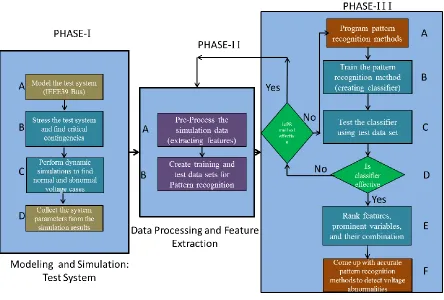
3.3 Methodology

As discussed in the previous sections, the main objective of this research is to detect

voltage collapse ahead of time. The methodology to achieve this objective consists of three

phases which are shown in the flow chart of Figure 3.1.

1. Modeling and simulation of test system: capture the power system dynamic response.

2. Data Processing and feature extraction: extract the system variables around the instance

of a disturbance that includes some pre-disturbance and post-disturbance variables.

(47)

Figure 3.1: Methodology flowchart for voltage stability prediction

3.3.1 Modeling and Dynamic Simulation of Test System (Phase-I)

Phase-I of the methodology discussed earlier in Section 3.2 is to capture the dynamic

response of the system. Here capturing the system response means recording the system

variables like bus voltage magnitudes, voltage angles, real and reactive powers, and generator

rotor angles. Dynamic response of the system can be captured by any one of the following two

methods,

(48)

– Model the equivalent system for dynamic simulations in power system simulation

tools such as PSSE.

– Perform the dynamic simulations on the modeled system using dynamic

simulation tools.

– Capture the system response for all the variables of the system

2. Collecting data from the field using PMUs

– Capture system data from the phasor measurement units (PMU) installed in the

substations. These PMUs will record system variables with time stamp

synchronized to GPS time clock.

To test the proposed methodology, this research utilized the IEEE 39 Bus equivalent system

in detecting voltage instability. This research can only use the first method from the above

mentioned two methods to capture the dynamic response on the test system. Flow chart shown in

Figure 3.1 shows all the steps involved in Phase-I.

Phase-I has four steps to capture the test system dynamic response. Test system is modeled

in Phase-I: Step A. Flow chart for this step is shown in Figure 3.2. In this step the equivalent

model data for the test system is collected from different articles and books, and is modeled in

power system dynamic simulation software such as PSSE. Multiple equivalent system models

are created with different types of loads like induction motor loads, composite load models, and

ZIP load models. Once the system models are built, a dynamic simulation is performed on the

(49)

Figure 3.2: Flow chart for Phase-I: Step-A

In Phase-I: Step-B, test system is stressed to determine critical contingencies by increasing

load or disconnecting generating plants or disconnecting transmission lines. Flow chart for

Phase-I: Step-B is shown in Figure 3.3. Contingency analysis is performed to determine the

critical contingencies, and from those contingencies voltage stable and voltage unstable cases

(50)

Figure 3.3: Flow chart for Phase-I: Step-B

After determining the critical contingencies, dynamic simulations are performed on

voltage stable and voltage unstable cases in Phase-I: Step-C using the power system dynamic

simulation software. Flow chart for Phase-I: Step-C is shown in Figure 3.4. Initially the base case

will be prepared for dynamic simulations, then dynamic simulations are performed on the

contingencies found in Phase-I: Step-B and system parameters are captured. Voltage stability is

determined from the dynamic simulations performed on each contingency. In Phase-I: Step-D

(51)

Figure 3.4: Flow chart for Phase-I: Step-C

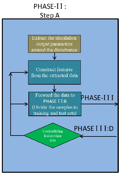
3.3.2 Data Processing and Feature Extraction (Phase-II)

Phase-II of the proposed methodology has two stages to pre-process the captured system

dynamic response for Phase-III. Flow chart shown in Figure 3.1 shows the stages for Phase-II.

Simulation parameters are extracted from the captured dynamic response of the system around

the disturbance. This extracted system variables have a few seconds of the system dynamic

response for pre-disturbance and post-disturbance data. Flow chart shown in Figure 3.5 shows

the process for Phase-II: Step-A. Multiple features are prepared from the extracted data. These

(52)

Figure 3.5: Flow chart for Phase-II: Step-A

3.3.3 Classification of Voltage Abnormality (Phase-III)

The last phase of the proposed methodology uses the pattern recognition techniques to

predict the voltage stability from the power system dynamic response. Flowchart for Phase-III is

shown in Figure 3.1. Algorithmic and statistical pattern recognition techniques are programmed

in this phase. These programmed methods are trained using the training samples extracted from

Phase-II and a classifier to predict voltage stability is developed from the pattern recognition

methods. This classifier is tested with the test samples extracted from Phase-II. If prediction

using the classifier is accurate and efficient, then the prominent features and prominent system

(53)

either the pattern recognition method or the training samples used to train the pattern recognition

method, are determined and corrected. In the last stage of Phase-III the accurate pattern

recognition methods to predict voltage collapse are determined.

3.4 Pattern Recognition

According to Duda and Hart [43], “pattern recognition is act of taking in raw data and

taking an action based on the category of the pattern”. A pattern is a type of reoccurring event or

object which can be named. Finger print image, hand written word, and speech are examples of a

pattern. The process of recognition is a machine classification and assigns the given objects to

prescribed classes. Figure 3.6 illustrates the flow chart pattern recognition model development

and data classification.

Pattern recognition techniques are used in engineering applications like wave form

classification where wave forms corresponding to one class of data are discriminated from the

data corresponding to a different class. We are using pattern recognition techniques to

distinguish voltage stable waveforms from voltage unstable waveforms. Regularized

least-squares (RLS) classification is used for our binary classification problem. RLSC is a learning

method that obtains solutions for binary classification problems.

By looking at Figure 3.6 it can be observed that pre-processing will take place on the

training set and test set acquired data and is forwarded to feature extraction purpose. Features

will be chosen on the given data. These selected features from the training set data are used to

build an optimized model for estimation. Later this model will be used to classify the patterns of

Predicting Voltage Abnormality Using Power System Dynamics

ScholarWorks@UNO

ScholarWorks@UNO

Predicting Voltage Abnormality Using Power System Dynamics

Predicting Voltage Abnormality Using Power System Dynamics

Predicting Voltage Abnormality Using

Power System Dynamics

Acknowledgements

Table of Contents

List of Figures

List of Tables

Abstract

Chapter 1

1

Introduction

1.1

Power System Stability

1.2

A Review of Voltage Stability

1.3

Review of Static Analysis Methods of Voltage Stability

1.4

Review of Dynamic Analysis Methods of Voltage Stability

1.5

Historical Review of Major Blackouts

1.6

Scope

Chapter 2

2

Methods of Voltage Stability Analysis

2.1

Static Voltage Stability Analysis methods

2.2

Dynamic Analysis

Chapter 3

3

Problem Statement, Objective, and Methodology

3.1

Problem Statement: Complications in Detecting Voltage Collapse

3.2

Objective

3.3

Methodology

3.4

Pattern Recognition