www.biogeosciences.net/12/7315/2015/ doi:10.5194/bg-12-7315-2015
© Author(s) 2015. CC Attribution 3.0 License.
New insights into
f
CO
2
variability in the tropical eastern
Pacific Ocean using SMOS SSS
C. Walker Brown, J. Boutin, and L. Merlivat
Sorbonne Universités (UPMC, Univ Paris 06)-CNRS-IRD-MNHN, LOCEAN Laboratory, 4 place Jussieu, 75005 Paris, France
Correspondence to: C. Walker Brown ([email protected])
Received: 5 January 2015 – Published in Biogeosciences Discuss.: 20 March 2015 Revised: 1 September 2015 – Accepted: 5 October 2015 – Published: 14 December 2015
Abstract. Complex oceanic circulation and air–sea interac-tion make the eastern tropical Pacific Ocean (ETPO) a highly variable source of CO2to the atmosphere. Although the
sci-entific community have amassed 70 000 surface fugacities of carbon dioxide (fCO2)data points within the ETPO region
over the past 25 years, the spatial and temporal resolution of this data set is insufficient to fully quantify the seasonal to interannual variability of the region, a region where fCO2
has been observed to fluctuate by > 300 µatm.
Upwelling and rainfall events dominate the surface phys-ical and chemphys-ical characteristics of the ETPO, with both yielding unique signatures in sea surface temperature and salinity. Thus, we explore the potential of using a statistical description offCO2within sea-surface salinity–temperature
space. These SSS/SST relationships are based on in situ sur-face ocean CO2 atlas (SOCAT) data collected within the
ETPO. This statistical description is then applied to high-resolution (0.25◦) Soil Moisture and Ocean Salinity (SMOS) sea surface salinity (SSS) and Operational Sea Surface Tem-perature and Sea Ice Analysis (OSTIA) sea surface tempera-ture (SST) in order to compute regional fCO2. As a result,
we are able to resolvefCO2at sufficiently high resolution to
elucidate the influence that various physical processes have on thefCO2of the surface ETPO.
Normalised (to 2014) oceanic fCO2 between July 2010
and June 2014 within the entire ETPO was 39 (±10.7) µatm supersaturated with respect to 2014 atmospheric par-tial pressures, and featured a CO2 outgassing of 1.51
(±0.41) mmol m−2d−1. Values of fCO2 within the ETPO
were found to be broadly split between the Gulf of Panama region and the rest of the tropical eastern Pacific Ocean. The northwest, central and offshore regions were supersaturated,
with wintertime wind-jet-driven upwelling found to consti-tute the first-order control onfCO2 values. This contrasts
with the southeastern/Gulf of Panama region, where heavy rainfall combined with rapid stratification of the upper water column act to dilute dissolved inorganic carbon, and yield fCO2values undersaturated with respect to atmospheric
fu-gacities of CO2.
1 Introduction
Perturbations to the global carbon cycle caused by anthro-pogenically driven increases in atmospheric partial pressures of CO2 (pCO2) produce an acute requirement to
under-stand inter-reservoir carbon fluxes (Le Quéré et al., 2015). However, assessing these fluxes, especially the flux between the atmosphere and surface ocean, is challenging, aspCO2
within the oceanic reservoir varies considerably both spa-tially and temporally. Fortunately, considerable effort has been made in recording oceanicpCO2(or fugacity –fCO2)
over the past 50 years, with roughly 10 million individual measurements of global surface ocean pCO2 taken,
pro-cessed, flagged and assembled into two large data sets: the surface ocean CO2atlas (SOCAT) and Lamont-Doherty
Earth Observatory (LDEO) carbon dioxide database (Bakker et al., 2014; Takahashi et al., 2014). Both databases make heavy use of “vessel-of-opportunity”-derivedpCO2data,
re-sulting in a heterogeneous data set with the majority of mea-surements collected within the tight confines of commercial shipping lanes.
pCO2observations over large areas of surface ocean.
Com-pleting a basic extrapolation of these vessel-of-opportunity-based data results in a spatially patchypCO2field, as seen
in the 1◦gridded product available from SOCAT (Bakker et al., 2014). Therefore, in order to achieve improved spatial coverage, a frequently used solution is to fit data-driven di-agnostic models (e.g. Feely et al., 2006; Park et al., 2010; Rödenbeck et al., 2013). These models use observed corre-lations between physical properties and thepCO2observed
under these conditions. In addition, statistical criteria, based on the surface ocean observations (for example, satellite im-agery) and/or neural networks, have been used to identify biogeochemical provinces in order to improve the accuracy of the extrapolated field (Boutin et al., 1999; Cosca et al., 2003; Rangama et al., 2005; Landschützer et al., 2014). Al-though the quality of these extrapolation methods has been refined over the past few years, in part due to the increasing number of in situ measurements, the interannual variability of the global air–sea CO2flux obtained using different
data-driven methods still substantially differs, and further work is required to unify our estimates and improve understanding of this air–sea flux.
The recent (2010–present) availability of sea surface salin-ity from the Soil Moisture Ocean Salinsalin-ity (SMOS) mis-sion has provided a new tool in statistically modelledpCO2
studies, as now the relationship between surface tempera-ture, salinity, density and pCO2 can be utilised in
high-resolution statistical descriptions of pCO2 within
tempera-ture and salinity (T S) space. It is this relationship that is ex-plored within this paper in order to quantify inter- and in-traannual variability within the oceanographically complex eastern tropical Pacific Ocean (ETPO) region between 4 and 18◦N, and east of 95◦W (Fig. 1).
[image:2.612.306.548.69.228.2]The ETPO region is influenced by northern and south-ern hemispheric trade winds, the doldrums, strong seasonal wind jets, heavy rainfall, strong solar heating and the El Niño–Southern Oscillation (ENSO; Kessler, 2006). Within the ETPO the intertropical tropical convergence zone (ITCZ) is neither zonally oriented, nor spatially fixed over the course of a year; thus wind fields are highly variable in both strength and direction (Kessler, 2006). Further wind variability is in-troduced by altitude jets blowing through three low-elevation gaps in the Central American Cordillera, with these jets observed predominantly between November and Febru-ary (Kessler, 2002, Fig. 1 – schematically represented by or-ange arrows). These strong jet winds are generated from the pressure gradient force resulting from high-pressure synoptic mid-latitude weather systems transiting North America to-wards the low-pressure equatorial Pacific during the winter months (Chelton et al., 2001). Jet wind velocities of up to 20–30 ms−1have been observed within the three gulfs, ex-tending from the shoreline to at least 500 km into the ETPO (Chelton et al., 2001). The alignment of these jets is mainly meridional in the Gulf of Panama and Tehuantepec, and more zonal in the Gulf of Papagayo (Fig. 1). These jet winds result
Figure 1. The topography of the eastern tropical Pacific Ocean and Isthmus of Panama, plotted using the General Bathymetric Chart of the Oceans (GEBCO; http://www.gebco.net/) bathymetry. The three gulfs within the region, Panama (84◦W from coastline of Panama), Papagayo (84 to 91◦W, north of 8◦N) and Tehuantepec (west of 91◦W, north of 10◦N), and the offshore region, are marked in white. The transect of WOCE cruise P19 is indicated in purple. The paths of jet winds are marked by orange arrows.
in strong wintertime upwelling in each of the three basins, with the northerly jet winds in the gulfs of Tehuantepec and Panama promoting Ekman upwelling (Kessler, 2006). At 9◦N, 90◦W, the quasi-permanent anticyclonic Costa Rica
thermocline dome is energised by the westerly jet winds in the Gulf of Papagayo, again, resulting in upwelling (Fig. 1; Kessler, 2002). However, the pressure disequilibrium that spawns these jet winds builds and subsides quickly (on a sub-weekly timescale), resulting in a highly fluctuating jet wind field, and non-linearities in the oceanic (and hence up-welling) response to these episodic events (Kessler, 2006). Recent studies have shown that satellite sea surface salin-ity (SSS) data are very well suited to capture the variabilsalin-ity of these high-SSS events (Grodsky et al., 2014; Reul et al., 2013).
2 Data and methods
2.1 Observations of in situfCO2, dissolved inorganic
carbon and atmospheric CO2
We use SOCAT data as the basis of a statistical description of pCO2 within the ETPO. All CO2 data within the
SO-CAT database are recorded as fugacity of CO2 (fCO2); a
measure ofpCO2that is corrected for the non-ideal-gas
be-haviour that carbon dioxide displays (Bakker et al., 2014). In this study we will use fugacity of CO2, owing to the
im-proved accuracy of this measure over pCO2. The logistical
importance of the region has proven beneficial, producing a large database offCO2/SSS/sea surface temperature (SST)
observations, with∼70 000 surface carbon, temperature and salinity data points collected between 1991 and 2011 (within the region depicted in Fig. 1). We use data (converted from pCO2tofCO2)collected between 1991 and 2013 within the
LDEO v2013 database as a semi-independent data set to test our SOCAT-based statistical description offCO2withinT S
space (Takahashi et al., 2014). The LDEO database extends 2 years longer than SOCAT, making it a useful evaluation product.
In addition to surface-fCO2, we use dissolved inorganic
carbon (DIC) concentrations within the ETPO measured dur-ing World Ocean Circulation Experiment cruise (WOCE) P19 in 1993 (Fig. 1; WOCE data available from http://cchdo. ucsd.edu/), and weekly dry-air CO2 mole fractions (xCO2)
measured at Fanning Island (3.5◦N, 159◦W; as part of the Scripps CO2program, http://scrippsco2.ucsd.edu/). We
de-rivefCO2in the atmosphere according to
fCO2 air=xCO2(patm−pH2O), (1) where Patm is the atmospheric pressure taken from the
ERA-Interim product (http://www.ecmwf.int/en/research/ climate-reanalysis/era-interim) and pH2O, the saturated wa-ter pressure (Weiss, 1974).
2.2 Calculating air–sea fluxes of CO2
The air–sea flux of CO2 (mmol m−2d−1) is derived using
the difference between surface ocean and atmosphericfCO2
values, the solubility of CO2in standard seawater (αCO2
cal-culated using the values given by Weiss, 1974) and the gas transfer velocitykCO2(cm h−1):
F =kCO2αCO2(fCO2 sea−fCO2 air). (2)
kis calculated using the 10 m wind-speed-based parameteri-sation described by Sweeney et al. (2007), where
k=0.27U2(660/Sc)0.5, (3)
where Sc is the Schmidt number for CO2 (Wanninkhof,
1992). We use the 0.25◦daily resolution 10 m wind speed product from the Advanced Scatterometer (ASCAT; www.
knmi.nl/scatterometer/) to calculate airfCO2, assuming
wa-ter vapour saturation at the boundary layer, then using the description in Eq. (1).
We note that when calculating air–sea gas exchange, it is not practical to derive a uniquekparameter for all oceanic conditions and locations of interest, therefore, through neces-sity,kis calculated using the non-specific parametrisation of Sweeney et al. (2007). Influences onk, such as rainfall, have been observed to enhance gas transfer velocities in laboratory experiments (Liss and Johnson, 2014). However, applying the results from these laboratory experiments into a modified gas transfer velocity within the ETPO region is challenging, and requires further field experiments to be validated. It is for this reason, and the role that rainfall has in reducing DIC, (thus bringing1fCO2closer to atmospheric equilibrium and
limiting the influence on air–sea fluxes brought about by an enhanced gas transfer velocity), we do not attempt to correct for the influence that rainfall has on air–sea exchanges.
2.3 Satellite observations of SST and SSS
Sea surface temperatures have been continuously measured from space via satellites since the AVHRR mission in 1981, and sea surface salinity has been measured since the launch of the European Space Agency’s Soil Moisture and Ocean Salinity (SMOS) satellite mission in November 2009 (Kerr et al., 2010). In this paper, we use satellite temperature (T) and salinity (S)data to help in the interpretation of spatial variability offCO2from the ETPO.
SMOS SSS maps at 0.25◦ resolution (running av-erage over 100×100 km2) produced by the LOCEAN SMOS group (combining SMOS ascending and de-scending passes) were used within this paper (Boutin et al., 2013, data available at catds.ifremer.fr/Products/ Available-products-from-CEC-OS/Locean-v2013). SMOS SSS data are not used prior to June 2010 due to variations in sensor configuration tested during the in-orbit sensor com-missioning phase (Corbella et al., 2011). Analysing the ac-curacy of the SMOS product, using in situ point observa-tions of SSS, can be completed using both SOCAT SSS data (where the salinity is derived from ship-mounted thermos-alinograph – TSG), and Argo profiles made within the re-gion (Appendix Fig. A1). Binning all Argo and TSG near-surface salinity data (that overlap the SMOS observational period) into the same monthly, 0.25◦structure as the SMOS monthly 0.25◦product, enables direct comparison. It is found
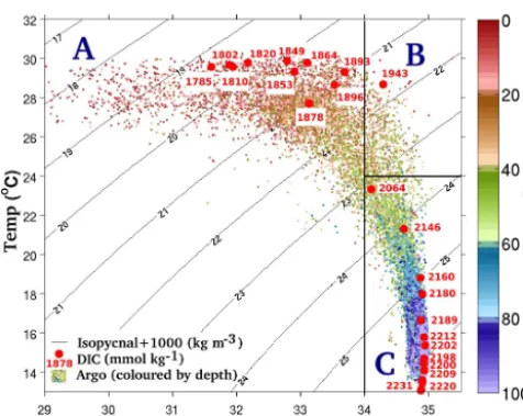
fea-Figure 2. The total library of Argo profiles collected within the ETPO in the upper 100 m. Numbered red dots indicate the total dissolved carbon concentration at specificT Svalues as measured during the WOCE cruise P19.
ture variabilities of 0.4 psu or higher (Delcroix et al., 2005). If the average intrinsic variability for the tropical Pacific (of 0.1 psu) is used, the measurement noise within the SMOS product is 0.14 psu. This measurement noise is included in our fCO2 error estimates (as detailed below). We suggest
that this is a satisfactory noise to signal ratio, given that the region features SSS variability of up to 8 psu (Fig. 2).
SSS was combined with sea surface temperatures from the Operational Sea Surface Temperature and Sea Ice Analysis (OSTIA) system; an optimal interpolation of multiple mi-crowave and infrared satellite-based data sources (Donlon et al., 2012). This SST daily product features a native resolu-tion of 0.05◦, which was subsequently re-sampled over the
same spatial and temporal grid as the SMOS data. As auxil-iary data sets for near-surface T andS, data from the Argo float array were used.
2.4 The basis of using a SST/SSS statisticalfCO2
model in the ETPO
Using anfCO2model based on surfaceT andSproperties
requires the carbon properties of water masses to be quanti-fied. We define three surface water masses within the study region, based on the near-surface (0–100 m depth)T andS characteristics of the ETPO recorded by∼6000 Argo pro-files between 17 and 4◦N, and east of 95◦W (Fig. 2). These water masses are also independently featured within studies by Kessler (2002, 2006):
1. an ETPO surface water, with temperatures > 27◦C and
salinities > 33.5 (Fig. 2, “B”);
2. deep water that predominantly exists below the thermo-cline (defined by Kessler as the 20◦C isotherm) and is
only expressed at the surface of the ETPO during peri-ods of upwelling (Fig. 2, “C”);
3. rain-influenced water, with salinities < 33.5 (Fig. 2, “A”).
Here, the water mass at C (herein referred to as “deep water”) is predominantly found at depths greater than 80 m, whilst the near-surface water is typically ETPO surface water and is warmer than 27.5◦C (A and B). Occasionally, the deep water mass can be observed at shallower depths, advected upwards during times of strong upwelling (Fig. 2). Rainfall-influenced waters display a wide range of salinities (from 29 to 34.5) within the upper 20 m (as observed in the salinity variation between A and B). At low salinities, densities as low as 1018 kg m−3 are observed – an 8 kg m−3 difference between this surface water and deep water (featuring densi-ties of 1026 kg m3). This large density gradient is an impor-tant feature of the ETPO, because in periods when stratifi-cation and high thermocline strengths are prevalent the up-welling of deep water is inhibited (Fiedler and Talley, 2006). To identify the carbon properties of these water masses, DIC concentrations between the surface and 100 m depth within the ETPO measured during the transect of WOCE P19 are shown as red circles and associated concentrations plot-ted withinT Sspace (Fig. 2). Deep water (C) was observed to have DIC concentrations > 2200 µmol kg−1 and contrasting values between A and B of < 1950 µmol kg−1. End-member
mixing occurs at intermediate temperatures between the two water masses B and C, exhibited in the gradient observed along the 34.2–34.75 isohalines in Fig. 2. Assuming that up-welling results in the expression of deep water at the surface, upwelling will act to increase the surface inventory of DIC, leading to increasedfCO2.
Rainfall results in surface layer dilution, thus reducing DIC between A and B (Turk et al., 2010). When thefCO2
of both end members in this system (rainwater and sur-face waters) are at equilibrium with the atmosphere, this dilution results in a lowering offCO2 within the sea
sur-face, and ingassing of CO2. Turk et al.’s (2010) study in
the western Pacific warm pool indicated that decreases of 30–40 µatm in surface-fCO2 values can result from
rain-fall alone, with these effects strongest under highly stratified conditions. This suggests that rainfall could be an important influence on ETPO fCO2, particularly within the
rainfall-dominated Panama Basin region. Finally, although biological processes influence DIC (and hencefCO2), observations of
[image:4.612.48.286.63.252.2]2.5 Processing SOCAT data
Surface fCO2 responds to changing levels of atmospheric
fCO2, which is increasing at approximately 20 µatm per
decade, (Takahashi et al., 2009, Fig. 3). In order to calcu-late contemporary air–sea fluxes, the multi-year SOCAT data must first be temporally corrected for the interannual trend of increasing atmospheric CO2. The mean annual increase in
fCO2 within the central equatorial Pacific (5◦N and 5◦S)
between 1979 and 1990 (excluding El Niño events) was es-timated at a rate of 1.1 µatm±0.3 per year (Takahashi et al., 2009). A second estimate, using data collected between 1990 and 2003 (within the region 10◦N to 5◦S) calculated an annual increase of 2.0 µatm±0.2 (Takahashi et al., 2009). Correcting 1991 data to contemporary July 2014 values would equate to a not-inconsiderable difference, depending on which of these two estimates was chosen. Therefore, in order to choose the optimum correction for the smaller sub-region of the ETPO, all available SOCATfCO2data 1991–
2011 were binned by year the data were collected (Fig. 3). Fitting a linear regression to the average bin value of this data resulted in an average annual increase of 1.95 µatm yr−1 (±0.38 µatm). This linear regression was found to fall within the 5th and 95th percentile values for all bins, with variability in mean and median values caused by heterogeneous sam-pling of the region and interannual variability (Fig. 3, per-centiles plotted in blue). Our calculated rate of increase is within the range of the annual atmospheric fCO2 increase
measured at Fanning Island (1.8 µatm yr−1±0.1 µatm), sug-gesting that fCO2 within the ETPO tracks the rate of
in-creasing atmosphericfCO2(Fig. 3). Therefore, we apply a
1.95 µatm per year correction to the SOCAT data in order to normalise thefCO2data to 1 July 2014 values, with all
re-sults herein also normalised to this date.
Although the spatial distribution offCO2SOCAT
[image:5.612.322.535.63.281.2]obser-vations within the ETPO is irregular, the variability can be constrained once theT Sproperties of the surface ocean are accounted for (as per DIC, Figs. 2, 4). Data from the upper 100 m of Argo profiles completed in each of the three gulfs (Panama, Papagayo and Tehuantepec, as defined in Fig. 1) show strongT S similarities between each of the three gulf regions; low-salinity (< 34) waters are observed in each gulf, with a thermocline separating surface water and deep water at 80–100 m depth. The T S properties of these Argo pro-files are replicated at the surface, within SOCAT SST and SSS data (Fig. 4). However, the relative number of observa-tions that fall into each water mass definition is different. The warm ETPO surface water is dominant in all three regions for the majority of samples, but cooler (< 20◦C) deep wa-ter is occasionally expressed at the surface, with this signal strongest in the Gulf of Tehuantepec, followed by the Gulf of Papagayo and seldom observed in the Gulf of Panama. This contrasts observations of low-salinity water, which are very frequent within the Gulf of Panama, but rare in the other two gulfs (Fig. 4). Although both SOCAT and Argo data suffer
Figure 3. Yearly binnedfCO2 measurements from the SOCAT database. The interpolated average rate of ETPOfCO2 increase
is shown as a red line, with the atmosphericfCO2data shown as
a green line. The blue boxes represent the 5th and 95th percentile
fCO2, with the small red lines indicating yearly averages, and the
red crosses indicating the yearly median.
from sparse sampling, we suggest that both data sets indicate that the relative dominance of each water mass within each of the three gulfs is different. There are very few SOCAT ob-servations within the offshore (OS) region (Fig. 1), thus we do not show aT Sdiagram from this region; however, Argo profiles from this region are included in Fig. 2, highlighting that the OS also shares the same water masses as the three gulf regions.
The distribution of DIC concentrations withinT Sspace is mirrored byfCO2values; deep water features higherfCO2
values than ETPO surface water, and low-salinity water fea-tures the lowest fCO2 values. The intermediate values of
fCO2 observed between each of these water masses
sug-gest end-member mixing offCO2 between water masses.
Finally, there are no water masses that shareT S characteris-tics, but feature very different DIC concentrations orfCO2
values, meaning that DIC/fCO2values are unique withinT S
space in this region (Figs. 2 and 4). Therefore, as both DIC andfCO2values behave pseudo-conservatively withinT S
space, it is possible to construct a statistical description of fCO2using solely SSS and SST.
2.6 Fitting a statistical description – the look-up table
The similarities of T, S and fCO2 properties of the
Figure 4.T Sdata from the three main gulfs within the ETPO both from Argo floats (coloured according to depth – top three plots) and from surface SOCATT andSdata, (coloured according to level offCO2– bottom three plots.
variance between individualfCO2observations occupying
the same location within T S space is low (Fig. 5b) we use a look-up table (LUT) to describefCO2as a function ofT
andS. This LUT technique, although not previously used to estimate oceanicfCO2, has proven useful for estimating net
primary productivity using satellite observations (Zhao et al., 2005). The LUT in this study uses a mesh of equal sized bins within T-S space. Observations of fCO2 within these
dis-creteT Sbins are collected, and an averagefCO2withinT S
space calculated. As each bin is fully independent of neigh-bouring bins, non-linear and/or skewed fCO2distributions
withinT S space – and hence an improved syntheticfCO2 product – can be accounted for with a lower attained root-mean-square error (RMSE) compared to using an alternative linear statistical description, such as a basic linear fit.
By combining all SOCAT data from the ETPO onto a sin-gle T-S diagram, a look-up table (LUT) can be produced in order to describe fCO2as a function of T andS (Fig. 5).
The LUT was constructed by completing a linear interpola-tion of binned 0.1 (salinity)×0.1◦C SOCAT data from the
entire ETPO region. The number of observations per bin is depicted in the right-hand panel. Here the highest number of observations fall in a narrow region of T S space, between
salinities of 32–34.5 and 25–30◦C (Fig. 5). We tested the quality of fit of the SOCAT-based LUT, using LDEO v2013 data. HerefCO2values were computed using the LUT and
usingT andS from the LDEO v2013 database, with these computed fCO2 data compared to the measured
(annual-increase-corrected)fCO2values. The LUT could be applied
to 96.2 % of all LDEO v2013 T-S measurements made be-tween 1990 and 2013, with the remainingT Smeasurements falling outside theT Sboundaries of the LUT.
The average root-mean-square error (RMSE) of the LUT was 16.8 µatm between the LUT computed and measured fCO2. This RMSE was asymmetrically distributed; it was
highest at temperatures of 22–26◦C/salinities of 34.4, and lowest at warmer temperatures/lower salinities and also at colder temperatures (Fig. 5). This suggests thatfCO2
vari-ability is low in aged surface waters, and high in recently upwelled and warming water. As there are a number of mea-surements within the region of higher error (Fig. 5), we hy-pothesise that this larger uncertainty is not due to lack of ob-servations, but rather to mixing/heating processes that allow water with slightly differentfCO2values to occupy the same
T Sspace. For example, thefCO2value of water at salinities
Figure 5. (a) The look-up table derived from the position of ETPO SOCATfCO2measurements withinT Sspace. (b) The
root-mean-square error of the LUT–fCO2 observations, showing the vari-ance between fCO2 observed within the same T S space in the
LUT. (c) The number of LDEO measurements per 0.1◦×0.1◦ salin-ity/temperature bins that went into generating the LUT.
mixing of two waters at salinities of 34.5, and temperatures of 18 and 32◦C, or solely from warmed 34.5/18◦C water. ThefCO2observed within the ETPO result from the
influ-ences of upwelling, solar radiation, horizontal advection, bi-ological productivity and diapycnal mixing. Therefore it is impossible to define a perfect relationship between the phys-ical attributes of the water and resulting fCO2
concentra-tion. However, this LUT technique works efficiently in de-termining the first-order variability of the system within the ETPO. In order to calculate the uncertainty of these LUT-derived syntheticfCO2data, we complete the mean-square
error calculation based on the variance offCO2data within
each cell of the LUT and the uncertainty of SMOS SSS (as described above.) We assume that the SST and SSS measure-ments within SOCAT and the OSTIA SST product are accu-rate. This error is propagated through the air–sea flux esti-mates in order to calculate the error of the air–sea flux values (as reported in Table 1).
3 Results
3.1 Bimonthly variability along ship paths
Bimonthly fCO2 variability can be seen in the (1991–
2011 annual- fCO2-increase-corrected) SOCAT
observa-tions plotted in Fig. 6. Here, the top six panels display SO-CAT observations offCO2, and the lower six panels display
fCO2 calculated from SOCAT SST and SSS observations
using the LUT. As the majority of SOCAT data are collected using ships of opportunity, resolution within shipping lanes in the ETPO is excellent; for example, multiple observations are made in regions south and west of the Panama Canal, at 9.1◦N, 79.7◦W, but are very sparse outside of these shipping lanes. However, though these issues in data resolution are ac-knowledged, patterns infCO2can still be detected. The
low-estfCO2is typically observed within the Gulf of Panama
and close to the coast. HigherfCO2is observed in the gulfs
of Tehuantepec and Papagayo. Interseasonal variability is also observed, with the highestfCO2 (> 440 µatm)
occur-ring between November and February, with lowerfCO2
val-ues (< 400 µatm) occurring across the entire region during the summer months (May–August). The data also show a very high degree of variability at small spatial and tempo-ral scales, for example during November–December within the Gulf of Papagayo. It is this variability that needs to be resolved using the LUT, when coupled to satellite SST and SSS observations at native resolution. Thus, it is important to confirm that the LUT is able to recreate this variability in fCO2using the initial (SOCAT)T andS conditions. Here,
we find that the LUT performs well, with most of the mea-suredfCO2variability also observed within thefCO2
cal-culated using the LUT (Fig. 6).
3.2 fCO2and fluxes by region – the influence of wind
and upwelling
Using the LUT, SMOS and OSTIA data, the small-scale vari-ability and features within the ETPO can be resolved more thoroughly than is possible through SOCAT data alone. Bi-monthly averaged (between July 2010 and June 2014) SSS, SST,fCO2, CO2flux and wind speed are plotted in Fig. 7.
Jet wind velocities over the Gulf of Tehuantepec are at their peak between October and February, thus optimising Ek-man upwelling. During these months the SSS of the gulf in-creases, whilst the SST decreases (due to the influences of upwelling). IncreasedfCO2is observed across most of the
Gulf of Tehuantepec, with peak outgassing occurring as a narrow band, centred underneath the axis of the jet wind. We suggest that this is due to the complimentary nature of ocean physics in this region – high wind speeds promote Ekman upwelling of high DIC deep water, whilst increasing the k component within the air–sea flux parameterisation, thereby maximising CO2outgassing.
4 Discussion
The Gulf of Papagayo shares many similarities with the Gulf of Tehuantepec; however, jet winds are more zonally aligned (reducing Ekman pumping strengths; Alexander et al., 2012), and occur later in winter compared to Tehuantepec, being strongest between November and February. This results in a lag between peak wintertimefCO2 values seen within the
two gulfs (Figs. 7 and 8). The Gulf of Papagayo also features elevatedfCO2values during the summer months which are
[image:7.612.50.289.66.186.2]Figure 6. SOCAT fCO2 bimonthly (January+February, March+April, May+June, July+August, September+October,
November+December) observations within the ETPO corrected for the annual CO2 increase, LUT-derived bimonthly fCO2
calcu-lated using SOCAT SST and SSS observations and LUT SOCAT observations.
The seasonally averaged wind velocities in the Gulf of Panama superficially resemble the wind patterns in the two northern gulfs – jet winds are observed between January and February (Fig. 7). However, excluding a small area of ocean directly underneath the wind jet axis during winter, the re-gion remains a small net sink of carbon throughout the year (Fig. 8). We suggest that this contrast between the Gulf of Panama and the rest of the ETPO is due to the high rain-fall within this region, resulting in the dilution of DIC as de-scribed above.
4.1 fCO2and the influence of rainfall
Figure 7. July 2010–June 2014 average SSS, SST, LUT-derived fCO, air–sea fluxes and wind vectors for the ETPO, split bimonthly (January+February, March+April, May+June, July+August, September+October, November+December).
stratification of the water column (Fig. 7, Alory et al., 2012). Qualitatively, this stratification can be observed in the SO-CAT and Argo data in Fig. 4 by the scarcity of deep water observations in the Gulf of Panama compared to the gulfs of Tehuantepec and Papagayo. Additionally, the thermocline is observed at deeper depths in the Argo profiles taken in the Gulf of Panama, compared to either the Gulf of Tehuantepec or Papagayo (Fig. 4).
The influence of stratification/rainfall on fCO2 values
is seen in Fig. 7. Here, the lowest salinity and fCO2 are
observed during the summer months (during peak rain-fall season; Alory et al., 2012). This low-fCO2, stratified
system persists until January, when intensification of the South Equatorial Current results in the export of the low-fCO2/fresh surface layer towards the southwest (as seen by
the elongation of the fresh pool during January–March SSS). This export of water, coupled with the dry season within the Gulf of Panama, appears to weaken the stratification, with the result that sporadic jet winds enable Ekman upwelling,
thus increasing SSS (Alory et al., 2012, Fig. 7) and average fCO2values between January and April (Fig. 8).
4.2 Air–sea fluxes from July 2010 to June 2014
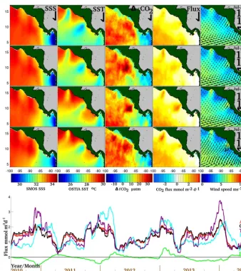
The ETPO between 2010 and June 2014 had an annual av-erage1fCO239.4 µatm (±10.7) and a outgassing CO2flux
of 1.51 mmol m−2d−1 (±0.41; Fig. 8/Table 1). The ETPO (the boundaries of which defined as per Fig. 1) has an area of 1.9×10¹²m2, therefore net outgassing from the ETPO equates to 10×1012g (0.01 Pg) of carbon per year.
Figure 8. Upper image: yearly average SSS, SST LUT-derived 1fCO2, air–sea fluxes and wind vectors for the ETPO for July to June
2010+2011, 2011+2012, 2012+2013 and 2013+2014. Lower image: the continuous LUT-derivedfCO2fluxes from the entire ETPO (red
line), the gulfs of Tehuantepec (purple), Papagayo (blue), Panama (green) and the South Equatorial Current (black).
Panama, which is a net sink of atmospheric CO2except
dur-ing occasional upwelldur-ing events durdur-ing January–February. However, ingassing within the Gulf of Panama is insufficient to offset outgassing from the rest of the ETPO, and the region remains a net source of CO2year round.
In addition to seasonal variability, interannual variability is observed within the ETPO. Across the entire basin, the ETPO during the years 2010–2012 were on average cooler and saltier than subsequent years (especially 2012–13). This resulted in higher annually averaged outgassing and fCO2
values (Fig. 8, Table 1). Concurrently, during 2010–2012, the Gulf of Panama featured a low-salinity mimima (of 28), and a small fresh pool footprint (the boundary of which is de-fined by the 33 isohaline; Alory et al., 2012). The extreme low salinity observed within the eastern region of the Gulf of Panama during 2010 to 2012 resulted in lowerfCO2and
hence stronger ingassing than 2012–2014 values,
highlight-ing the effect of rainwater dilution of DIC. However, this lo-calised ingassing was insufficient to offset the higher out-gassing observed in the other regions of the ETPO (Fig. 8, Table 1). Also noteworthy is that average wind velocities were similar during 2010 and 2012 compared to subsequent years, so the increased outgassing observed during these years cannot be attributed to increased wind-mediated Ek-man upwelling of deep water alone.
We note that the period of 2010 to the end of 2011 featured La Niña conditions, and suggest that this could be causal to the differences in CO2 fluxes, higher salinities and higher
fCO2observed during this time period. A study using NCEP
col-umn by intensified coastal Kelvin waves. Mechanistically, this shallow thermocline reduces the strength of upwelling required for the expression of deep water at the surface, thus decreasing average SSTs observed during La Niña periods (Alexander et al., 2012).
Furthermore, a study by Alexander et al. (2012) also sug-gests that although jet winds are the first-order control on SST and thermocline depth during winter, it is changes in the thermocline depth (rather than changes in jet winds) that re-sult in observed El Niño–Southern Oscillation (ENSO) vari-ability in SST within the ETPO. Varivari-ability in thermocline depth, and by association, variability in the ease by which deep water can be advected towards the surface, suggests that the ENSO could drive variability within the surface-fCO2
observations. However, with only 4 years of data, and no El Niño phase for intercomparison, we are unable to draw definitive conclusions.
4.3 Previous work
The results in Figs. 7 and 8 represent the first attempt to quantify fCO2 within the ETPO region at high resolution
using observations. Previous work encompassing the ETPO includes three basin-wide or globalfCO2/pCO2studies, by
Takahashi et al. (2009), Ischii et al. (2014) and Landschützer et al. (2014). These studies, as discussed in the introduction, are based on the extrapolation ofpCO2 directly, or the
ex-trapolation ofpCO2using a neural network technique, and
feature spatial resolutions of 4◦×5◦, 4◦×5◦ and 1◦×1◦ respectively. Of these three studies, only the study by Taka-hashi et al. (2009) features a data set of calculated1pCO2
that includes the ETPO region, thus allowing direct compar-ison with our calculations. Collocating the 1pCO2 results
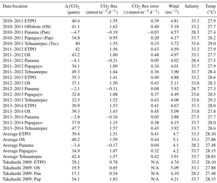
from Takahashi et al. (2009) within the ETPO regions de-fined in Fig. 1, the gulfs of Tehuantepec, Papagayo, Panama and the offshore region featured values of +28.9, +54.1, +17.1 and+19.5 µatm respectively (Table. 1). This suggests that the Takahashi et al. (2009) study differentiates the low 1pCO2Gulf of Panama region from the higher values
ob-served in the gulfs of Tehuantepec and Papagayo. The reso-lution used in Takahashi’s study is too coarse to identify any mesoscale features (such as upwelling), or interannual vari-ability within the region. However, we find that an average 1pCO2value from Takahashi et al. (2009) of 29.1 µatm was
within the error limits of this study (Table 1).
Applying the same wind speed product and gas transfer parametrisation used in this study to the ETPO1pCO2
val-ues from Takahashi et al. (2009), we find that all regions are outgassing, with the Gulf of Papagayo dominant within the ETPO (Table 1). The ingassing observed within the Gulf of Panama for our study is not replicated in Takahashi et al. (2009). The improved resolutions featured in Land-schützer et al. (2014) resulted in some mesoscale features being observed, such as the increased pCO2values within
the Gulf of Papagayo. However, this work was not able to
identify the lowpCO2conditions within the Gulf of Panama,
most likely due to the same biogeochemical province de-scription being applied to the entire ETPO. In addition to these studies, our work distinguishes the importance of jet winds in increasingpCO2, and quantifies the strong
interan-nual variability within the region.
5 Conclusions
Estimating surface-fCO2and air–sea fluxes of CO2within
the global oceans has advanced considerably over the past decade, assisted by the assembly of large standardised at-lases of surface observations (such as the SOCAT database). However, although these databases boast measurements in the millions, a challenge remains in gauging seasonal or sub-mesoscalefCO2variability in the oceans. Sampling through
the use of commercial volunteering observation vessels may introduce bias, with most data existing within the narrow confines of the major global shipping lanes or for only a few months of the year. However, the quantification of fCO2
withinT S space, used in conjunction with observations of surface SST and SSS (made possible through the recent availability of SSS data from satellites), has proved highly useful in improving our understanding offCO2variability
at much improved spatial and temporal resolutions. We have demonstrated a technique using SOCAT data to identify the fCO2signatures of water masses within the ETPO region,
namely, the high fCO2 deep water, the near-equilibrium
ETPO surface water and the undersaturated rainfall diluted surface waters. From this, we used a LUT technique to pro-duce a description of the fCO2 content of ETPO surface
water using satellite SST and SSS data. The highest out-gassing and surface-fCO2values were observed during the
winter period (November–March), in the gulfs of Tehuante-pec, Papagayo and in the South Equatorial Current. The first-order control on these upwelling events, and hencefCO2in
the ETPO, are strong wind jets blowing through low-altitude gaps in the Central American cordillera. The Gulf of Panama remained undersaturated on average, due to dilution effects of heavy rainfall and the stratification of the water column. Although wind jets were observed in the Gulf of Panama, the exceptionally low density of the water within this region appears to limit upwelling, and any upwelling that occurs is directly underneath the wind jet axis. Inter-annual vari-ability was observed within the region, with the location of the western extent of the fresh pool moving considerably westwards between 2010 and 2014. Previous work within this region suggests that changes in thermocline depth re-lated to ENSO are likely to influencefCO2within this
re-gion. The region is a net contributor to atmospheric CO2,
Appendix A
Table A1. Annual averaged values for each region, as reported in Fig. 8, and average values from Takahashi et al. (2009).
Date/location 1fCO2 CO2flux CO2flux error Wind Salinity Temp
(µatm) (mmol m−2d−1) (±mmol m−2d−1) (ms−2) (◦C) 2010–2011 ETPO 40.4 1.55 0.39 4.81 33.3 27.9 2010–2011 Offshore (OS) 41.1 1.62 0.40 5.18 33.2 27.7 2010–2011 Panama (Pan) −4.7 −0.19 −0.03 4.57 28.3 27.4 2010–2011 Papagayo (Pap) 34.8 0.95 0.20 4.17 33.7 28.2 2010–2011 Tehuantepec (Tec) 40 1.55 0.33 3.72 33.6 29.0 2011–2012 ETPO 42 1.56 0.43 4.59 33.3 27.9 2011–2012 OS 43.2 1.60 0.48 4.97 33.1 27.7 2011–2012 Panama −4.1 −0.21 0.05 4.02 28.4 27.5 2011–2012 Papagayo 34.1 1.09 0.34 4.01 33.7 27.9 2011–2012 Tehuantepec 49.3 1.64 0.36 3.90 33.7 28.4 2012–2013 ETPO 35.3 1.41 0.40 4.88 33.2 28.6 2012–2013 OS 37.1 1.50 0.43 5.11 33.0 28.3 2012–2013 Panama −2.1 −0.11 0.08 3.92 28.7 27.3 2012–2013 Papagayo 32.8 1.08 0.37 4.49 33.6 28.5 2012–2013 Tehuantepec 32.5 1.52 0.43 4.08 33.6 29.3 2013–2014 ETPO 39.9 1.53 0.41 4.67 33.3 28.0 2013–2014 OS 39.3 1.63 0.45 5.09 33.0 27.8 2013–2014 Panama −2.8 −0.16 0.05 3.88 27.5 27.7 2013–2014 Papagayo 37.9 1.15 0.38 4.15 33.7 28.0 2013–2014 Tehuantepec 47.7 1.57 0.43 3.92 33.7 28.6 Average ETPO 39.4 1.51 0.41 4.7 33.3 28.10
Average OS 40.2 1.59 0.44 5.1 33.1 27.88
Acknowledgements. The research leading to these results was aided by the LOCEAN team Xiaobin Yin and Nicolas Martin, and supported through the EU FP7 project CARBOCHANGE – Changes in carbon uptake and emissions by oceans in a changing climate – which received funding from the European Commis-sion’s Seventh Framework Programme under grant agreement no. 264879, and the SMOS+SOS STSE project funded by the ESA. We would also like to thank all of the contributors to SOCAT and LDEO of fCO2/pCO2 observations within the Pacific Ocean,
specifically Yukihiro Nojiri, Taro Takahashi and Richard Feely who contributed greatly within this region. Finally, we would like to thank the anonymous reviewer and Rik Wanninkhof for their insightful reviews.
Edited by: F. Chai
References
Alexander, M. A., Seo, H., Xie, S. P., and Scott, J. D.: ENSO’s Im-pact on the Gap Wind Regions of the Eastern Tropical Pacific Ocean, J. Clim., 25, 3549–3565, 2012.
Alory, G., Maes, C., Delcroix, T., Reul, N., and Illig, S.: Sea-sonal dynamics of sea surface salinity off Panama: The far Eastern Pacific Fresh Pool, J. Geophys. Res., 117, C04028, doi:10.1029/2011JC007802, 2012.
Bakker, D. C. E., Pfeil, B., Smith, K., Hankin, S., Olsen, A., Alin, S. R., Cosca, C., Harasawa, S., Kozyr, A., Nojiri, Y., O’Brien, K. M., Schuster, U., Telszewski, M., Tilbrook, B., Wada, C., Akl, J., Barbero, L., Bates, N. R., Boutin, J., Bozec, Y., Cai, W.-J., Castle, R. D., Chavez, F. P., Chen, L., Chierici, M., Cur-rie, K., de Baar, H. J. W., Evans, W., Feely, R. A., Fransson, A., Gao, Z., Hales, B., Hardman-Mountford, N. J., Hoppema, M., Huang, W.-J., Hunt, C. W., Huss, B., Ichikawa, T., Johan-nessen, T., Jones, E. M., Jones, S. D., Jutterström, S., Kitidis, V., Körtzinger, A., Landschützer, P., Lauvset, S. K., Lefèvre, N., Manke, A. B., Mathis, J. T., Merlivat, L., Metzl, N., Murata, A., Newberger, T., Omar, A. M., Ono, T., Park, G.-H., Pater-son, K., Pierrot, D., Ríos, A. F., Sabine, C. L., Saito, S., Salis-bury, J., Sarma, V. V. S. S., Schlitzer, R., Sieger, R., Skjelvan, I., Steinhoff, T., Sullivan, K. F., Sun, H., Sutton, A. J., Suzuki, T., Sweeney, C., Takahashi, T., Tjiputra, J., Tsurushima, N., van Heuven, S. M. A. C., Vandemark, D., Vlahos, P., Wallace, D. W. R., Wanninkhof, R., and Watson, A. J.: An update to the Surface Ocean CO2Atlas (SOCAT version 2), Earth Syst. Sci. Data, 6,
69–90, doi:10.5194/essd-6-69-2014, 2014.
Boutin, J., Etcheto, J., and Dandonneau, Y.: Satellite sea surface temperature: a powerful tool for interpreting in situpCO2 mea-surements in the equatorial Pacific Ocean, Tellus B, 51B, 490– 508, 1999.
Boutin, J., Martin, N., Reverdin, G., Yin, X., and Gaillard, F.: Sea surface freshening inferred from SMOS and ARGO salinity: im-pact of rain, Ocean Science, 9, 183–192, doi:10.5194/os-9-183-2013, 2013.
Chelton, D. B., Esbensen, S. K., Schlax, M. G., Thum, N., Freilich, M. H., Wentz, F. J., and Schopf, P. S.: Observations of coupling between surface wind stress and sea surface temperature in the eastern tropical Pacific, J. Climate, 14, 1479–1498, 2001.
Corbella, I., Torres, F., Duffo, N., González-Gambau, V., Pablos, M., Duran, I., and MartínNeira, M.: MIRAS Calibration and Performance: Results From the SMOS In-Orbit Commissioning Phase, IEEE Trans. Geosci. Remote Sens., 49, 3147–3155, 2011. Cosca, C. E., Feely, R. A., Boutin, J., Etcheto, J., McPhaden, M. J., Chavez, F. P., and Strutton, P. G.: Seasonal and interannual CO2fluxes for the central and eastern equatorial Pacific Ocean
as determined fromfCO2-SST relationships, J. Geophys.
Res.-Oceans, 108, 3278, doi:10.1029/2000JC000677, 2003.
Delcroix, T., McPhaden, M. J., Dessier, A., and Gouriou, Y.: Time and space scales for sea surface salinity in the tropical oceans, Deep-Sea Res. Pt. I, 52, 787–813, doi:10.1016/j.dsr.2004.11.012, 2005.
Donlon, C. J., Martin, M., Stark, J., Roberts-Jones, J., Fiedler, E., and Wimmer, W.: The operational sea surface temperature and sea ice analysis (OSTIA) system, Remote Sens. Environ., 116, 140–158, 2012.
Feely, R. A., Takahashi, T., Wanninkhof, R., McPhaden, M. J., Cosca, C. E., Sutherland, S. C., and Carr, M. E.: Decadal vari-ability of the air-sea CO2fluxes in the equatorial Pacific Ocean, J.
Geophys. Res.-Oceans, 111, doi:10.1029/2005JC003129, 2006. Fiedler, P. C. and Talley, L. D.: Hydrography of the
east-ern tropical Pacific: A review, Prog. Oceanogr., 69, 143–180, doi:10.1016/j.pocean.2006.03.008, 2006.
Grodsky, S. A., Carton, J. A., and Bentamy, A.: Salty anomalies forced by Tehuantepec and Papagayo gap winds: Aquarius observations, Remote Sens. Lett., 5, 568–574, doi:10.1080/2150704X.2014.935522, 2014.
Ishii, M., Feely, R. A., Rodgers, K. B., Park, G.-H., Wanninkhof, R., Sasano, D., Sugimoto, H., Cosca, C. E., Nakaoka, S., Telszewski, M., Nojiri, Y., Mikaloff Fletcher, S. E., Niwa, Y., Patra, P. K., Valsala, V., Nakano, H., Lima, I., Doney, S. C., Buitenhuis, E. T., Aumont, O., Dunne, J. P., Lenton, A., and Takahashi, T.: Air-sea CO2flux in the Pacific Ocean for the period 1990–2009,
Biogeo-sciences, 11, 709–734, doi:10.5194/bg-11-709-2014, 2014. Kerr, Y. H., Waldteufel, P., Wigneron, J. P., Delwart, S., Cabot, F. O.,
Boutin, and Escorihuela, M.: The SMOS mission: New tool for monitoring key elements of the global water cycle, Proc. IEEE, 98, 666–687, 2010.
Kessler, W.: Mean three-dimensional circulation in the northeast tropical Pacific, J. Phys. Oceanogr., 2457–2471, 2002.
Kessler, W. S.: The circulation of the eastern tropical Pacific: A re-view, Prog. Oceanogr., 69, 181–217, 2006.
Landschützer, P., Gruber, N., Bakker, D. C. E., and Schuster, U.: Recent variability of the global ocean carbon sink, Global Bio-geochem. Cy., 28, 927–949, 2014.
N.: Global carbon budget 2014, Earth Syst. Sci. Data, 7, 47–85, doi:10.5194/essd-7-47-2015, 2015.
Liss, P. and Johnson., M.: Ocean-Atmosphere Interactions of Gases and Particles, Springer-Verlag, Berlin, 55–112, 2014.
Park, G.-H., Wanninkhof, R. I. K., Doney, S. C., Takahashi, T., Lee, K., Feely, R. A., Sabine, C. L., Triñanes, J., and Lima, I. D.: Variability of global net sea–air CO2fluxes over the last three
decades using empirical relationships, Tellus B, 62, 352–368, doi:10.1111/j.1600-0889.2010.00498.x, 2010.
Rangama, Y., Boutin, J., Etcheto, J., Merlivat, L., Takahashi, T., Delille, B., Frankignoulle, M., and Bakker, D. C. E.: Variabil-ity of the net air–sea CO2 flux inferred from shipboard and
satellite measurements in the Southern Ocean south of Tasma-nia and New Zealand, J. Geophys. Res.-Oceans, 110, C09005, doi:10.1029/2004JC002619, 2005.
Reul, N., Fournier, S., Boutin, J., Hernandez, O., Maes, C., Chapron, B., Alory, G., Quilfen, Y., Tenerelli, J., Morisset, S., Keer, Y., Mecklenburg, S., and Delwart, S.: Sea Surface Salin-ity Observations from Space with the SMOS Satellite: A New Means to Monitor the Marine Branch of the Water Cycle, Surv. Geophys., 35, 681–722, doi:10.1007/s10712-013-9244-0, 2013. Rödenbeck, C., Keeling, R. F., Bakker, D. C. E., Metzl, N., Olsen,
A., Sabine, C., and Heimann, M.: Global surface-oceanpCO2
and sea–air CO2 flux variability from an observation-driven
ocean mixed-layer scheme, Ocean Sci., 9, 193–216, 2013, http://www.ocean-sci.net/9/193/2013/.
Sweeney, C., Gloor, E., Jacobson, A. R., Key, R. M., McKinley, G., Sarmiento, J. L., and Wanninkhof, R.: Constraining global air-sea gas exchange for CO2with recent bomb14C measurements,
Global Biogeochem. Cy., 21, doi:10.1029/2006GB002784, 2007.
Takahashi, T., Sutherland, S. C., Wanninkhof, R., Sweeney, C., Feely, R. A., Chipman, D. W., and De Baar, H. J.: Climatolog-ical mean and decadal change in surface oceanpCO2, and net sea–air CO2flux over the global oceans, Deep-Sea Res. Pt. II,
56, 554–577, 2009.
Takahashi, T., Sutherland, S. C., Chipman, D. W., Goddard, J. G., and Ho, C.: Climatological distributions of pH,pCO2, total CO2,
alkalinity, and CaCO3saturation in the global surface ocean, and
temporal changes at selected locations, Mar. Chem., 164, 95– 125, 2014.
Turk, D., Zappa, C. J., Meinen, C. S., Christian, J. R., Ho, D. T., Dickson, A. G., and McGillis, W. R.: Rain impacts on CO2
ex-change in the western equatorial Pacific Ocean, Geophys. Res. Lett., 37, doi:10.1029/2010GL045520, 2010.
Wanninkhof, R.: Relationship between wind speed and gas ex-change, J. Geophys. Res, 97, 7373–7382, 1992.
Weiss, R. F.: Carbon dioxide in water and seawater: The solubility of a nonideal gas, Mar. Chem., 2, 203–215, 1974.
Xie, S.-P., Xu, H., Kessler, W. S., and Nonaka, M.: Air–Sea Inter-action over the Eastern Pacific Warm Pool: Gap Winds, Ther-mocline Dome, and Atmospheric Convection, J. Clim., 18, 5–20, 2005.