www.ann-geophys.net/26/2999/2008/ © European Geosciences Union 2008
Annales
Geophysicae
Diagnostic of the temperature and differential emission measure
(DEM) based on Hinode/XRT data
M. Siarkowski1, R. Falewicz2, A. Ke¸pa1, and P. Rudawy2
1Space Research Centre, Polish Academy of Sciences, 51-622 Wrocław, ul. Kopernika 11, Poland 2Astronomical Institute, University of Wrocław, 51-622 Wrocław, ul. Kopernika 11, Poland
Received: 10 October 2007 – Revised: 21 April 2008 – Accepted: 24 April 2008 – Published: 15 October 2008
Abstract. We discuss here various methodologies and an optimal strategy of the temperature and emission measure diagnostics based on Hinode X-Ray Telescope data. As an example of our results we present the determination of the temperature distribution of the X-rays emitting plasma us-ing a filters ratio method and three various methods of the calculation of the differential emission measure (DEM). We have found that all these methods give results similar to the two filters ratio method. Additionally, all methods of the DEM calculation gave similar solutions. We can state that the majority of the pairs of the Hinode filters allows one to derive the temperature and emission measure in the isother-mal plasma approximation using standard diagnostics based on the two filters ratio method. In cases of strong flares one can also expect good conformity of the results obtained using a Withbroe – Sylwester, genetic algorithm and least-squares methods of the DEM evaluation.
Keywords. Solar physics, astrophysics, and astronomy (Corona and transition region; Ultraviolet emissions; X rays and gamma rays; Instruments and techniques)
1 Introduction
The solar corona with temperatures greater than one mil-lion degrees emits mainly in the X-ray domain of the spec-trum. Its emission contains both the continuum from thermal plasma and the line emission of highly ionized elements. The earliest phases of solar flares are dominated by non-thermal emissions (hard X-rays), the remainder of the events man-ifests itself primarily by thermal emissions at wavelengths ranging from X-rays through visual. The thermal radiation comes from plasma having a wide range of temperatures.
Temperature and emission measure diagnostics of the ac-tive region and flaring loops are very important to model the
Correspondence to: M. Siarkowski
loop structures, and analyze the heating sources and their (heating) distribution along the loop.
For the optically thin emission, assuming isothermal plasma temperature, the well known method of filter ratio, based on the ratio of the observed fluxes in two selected en-ergy (or wavelengths) bands (Vaiana et al., 1973; Thomas et al., 1985) can be used. In the case of multi-temperature plasma the filter ratio method derives the line-of-sight aver-age isothermal temperature and emission measure. There-fore, in this approach it is more adequate to use many fil-ters or lines in terms of differential emission measure distri-butions DEM(T )/dT (Pottash et al., 1964; Sylwester et al., 1980). Extended discussion of the DEM versus isothermal approximation can by found, for example, in Schmelz et al. (2001), Cirtain et al. (2007) and references therein.
Hinode is a new advanced optical, UV and X-ray solar
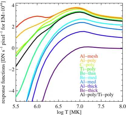
5.5 6.0 6.5 7.0 7.5 8.0 log T [MK]
−4 −2 0 2 4
response functions [DN s
−1 pixel −1 for EM=10 44 ]
Al−mesh
Al−poly C−poly Ti−poly
Be−thin
Be−med
Al−med
Al−thick
[image:2.595.63.271.63.253.2]Be−thick Al−poly/Ti−poly
Fig. 1. Theoretical temperature response functions of the selected XRT filters.
In this paper we will check if the XRT response character-istics allow diagnostics of temperature (T) and emission mea-sure (EM) of the coronal plasma. We also describe the ob-servations selected for the analysis. Additionally, we present and discuss the filters ratio method in isothermal approxi-mation and three different methods for differential emission measure (DEM) analysis in multi-temperature approxima-tion, respectively.
In all calculations we used the temperature response func-tion as given by SolarSoft and presented in Fig. 1.
2 Data analysis
For our work we selected three typical X-ray emitting ac-tive regions observed by Hinode/XRT with 6 or more dif-ferent filters. To prepare the selected data we used standard SolarSoft routine xrt prep.pro, which is similar in nature to
sxt prep.pro (Yohkoh software). This routine converts raw
data into index and structure arrays. Additionally, this pro-cess removes several instrumental effects. We could men-tion some of the most important, for example: replacement of the near-saturated pixels for a value greater than 2500 DN with 2500 DN, remove radiation-belt/cosmic-ray and streaks, calibration for read-out signals, removing of the CCD bias, calibration of the dark current, normalization of each image for exposure time. Using processed data we calculated their differential emission measure distributions and using a two filters ratio method, temperature and emission measure maps in isothermal approximation.
2.1 Two filters ratio diagnostic
The filter-ratio method is a technique commonly used for plasma diagnostics based on data from broad-band X-ray imaging systems. This method requires analysis of two or more intensity maps (images) of the investigated structures obtained with various broad-band filters. It delivers maps of temperatures and line-of-sight emission integrals or emission measure distributions as a function of temperature.
For a multi-band instruments like XRT, under the assump-tion that the emitting plasma is optically thin, the observed fluxFk in filterkin a single pixel is:
Fk = Z
T Z
λ
f (T , λ)ηk(λ)EM(T )dλdT , (1)
wheref (T , λ)is coronal plasma emissivity as a function of the plasma temperatureT and the wavelengthλ, calculated at a distance of 1 AU using a CHIANTI spectral code (includ-ing both emission lines and continuum).ηk(λ)is an effective area of the instrument which includes the geometric area and the reflectance of the telescope mirror, the entrance and the focal plane filter transmissions and the CCD quantum effi-ciency. EM(T) is a collection of emission measures over a range of temperatures located along the line of sight. Defin-ing the temperature response functionPk(T) of filter k as a convolution of the instrument effective areaηkand emissiv-ity of solar plasmaf:
Pk = Z
λ
f (T , λ)ηk(λ)dλ, (2)
we can rewrite Eq. (1) as:
Fk = Z
T
Pk(T )EM(T )dT ≈ X
i
Pk(Ti)EM(Ti). (3)
For isothermal approximation this equation can be written as:
Fk =Pk(T )EM(T ). (4)
Similar to Thomas et al. (1985) using Eq. (4) one can calcu-late ratioRof the observed fluxes (F) in two filters labeled “1” and “2” for a co-aligned pixel area. This can be written as:
R(T )= F1
F2
=P1(T )
P2(T )
. (5)
According to Eq. (5), the ratioRof observed fluxes depends on plasma temperatureT only. In the next step, one can cal-culate the emission measureEM(T )=Fk/Pk(T ).
This procedure can be used on all combinations of the XRT filters, but it has a limited usability. In particular, ra-tioRcan be sometimes an ambiguous function in the whole range of temperatures.
Fig. 2. Temperature and emission measure maps calculated from two filters ratio, Al poly/Al thick for the active region NOAA 0955 observed on 13 May 2007 at 17:57:30 UT.
2.2 Analysed events
The first analysed region was a relatively faint active region NOAA 0955. Observations were made on 13 May 2007 at around 18:00 UT. Images taken in a ten filters combina-tion are available. Temperature and emission measure maps were calculated using two pairs of filters, Al poly/Al thick and Ti poly/Al thick. As an example the resulted maps for the Al poly/Al thick pair are presented in Fig. 2. For both pairs of filters the filter ratios are sensitive for tem-peratures from log(T )=6.1 up to log(T )=7.7. However, for all structures of this quiet active region we obtained temperatures in the ranges 2.0–3.3 MK and 1.8–2.4 MK for the Al poly/Al thick and Ti poly/Al thick pairs, respec-tively. The range of the observed temperatures is typical for solar quiet active regions (see, e.g. Golub and Pasachoff, 1997).
An active region NOAA 0923 was seen on the edge of the West solar limb between 19 and 23 Novem-ber 2006. Observations analyzed here were made on 20 November 2006 at around 21:16 UT. Images taken in six filters are available. Temperature and emission measure maps were calculated for two pairs of filters: Al poly/Al mesh and Al poly/Be thin. The resulting maps for the Al poly/Be thin filters pair are presented in Fig. 3. The highest temperatures in the range of 3.5 MK are observed in the brightest loop, seen just on the solar limb.
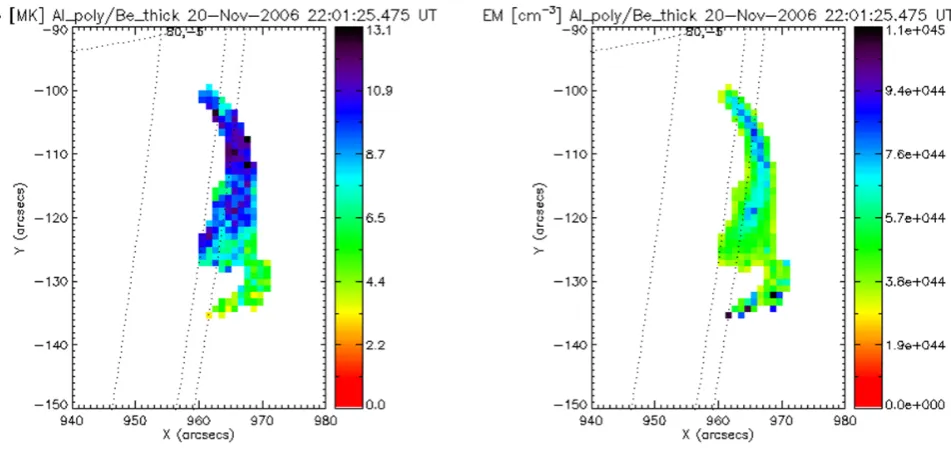
The same active region NOAA 0923 was observed one hour later with seven filters. Temperature and emission measure maps were calculated for two pairs of filters:
Al poly/Al mesh and Al poly/Be thick. The resulted maps for the Al poly/Be thick pair are shown in Fig. 4.
Due to the construction of the filter wheels, XRT images in various filters are only obtained consecutively. Thus an important assumption underlying the filters ratio diagnostic (and also DEM analysis described below) is that there was no substantial change in the morphology and energetics of the event between two images using various filters. This as-sumption is usually fulfilled in the case of quiet Sun and ac-tive region observations. Checking the light-curves for dif-ferent filters we proved that this assumption is also true in the observations above described. Moreover, in the case of the small B1.5 flare images with different filters were obtained first around the maximum and the second one in decay phase of the event. We use this pair because the second filter had only one “thick” filter available. The exact co-alignment of the images is likewise important, especially for the DEM cal-culations in the individual pixels.
Using a “harder” Al poly/Be thick filters pair instead of a “softer” Al poly/Be thin pair results in obtaining much higher temperatures. Temperatures in the brightest loop reached average values up to∼13 MK. Such a high tempera-ture could be connected to the appearance of a small B1.5 class solar flare observed in this active region. The flare started at 22:00 UT, reached its maximum at 22:05 UT and ended at 22:09 UT. In fact, the temperature obtained from
GOES data for this small flare reached the value around
10 MK.
Fig. 3. Temperature and emission measure maps calculated from two filters ratio, Al poly/Be thin for the active region NOAA 0923 observed on West solar limb on 20 November 2006 at 21:16:19 UT.
Fig. 4. Temperature and emission measure maps calculated from two filters ratio, Al poly/Be thick for the active region NOAA 0923 observed on West solar limb on 20 November 2006 at 22:01:25 UT.
where fluxes can vary rapidly it is possible, in principle, to interpolate the intensities of one image to match the time at which the image in the other filter was acquired. Examples of temperature and DEM analysis of solar flares are well known in the case of Yohkoh observations (McTiernan et al., 1999). Examples of DEM analysis with Hinode/XRT in the GOES C8.2 flare is presented by Reeves et al. (2007).
2.3 Distribution of the Differential Emission Measure
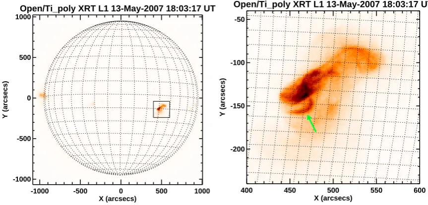
[image:4.595.69.545.347.573.2]Open/Ti_poly XRT L1 13-May-2007 18:03:17 UT
-1000 -500 0 500 1000
X (arcsecs) -1000
-500 0 500 1000
Y (arcsecs)
Open/Ti_poly XRT L1 13-May-2007 18:03:17 UT
400 450 500 550 600
X (arcsecs) -200
-150 -100 -50
[image:5.595.78.510.64.271.2]Y (arcsecs)
Fig. 5. On the left: full Sun image obtained by XRT/Hinode with Ti poly filter. On the right: enlarged map of NOAA 955 active region observed by Hinode/XRT telescope with Ti poly filter. The DEM distribution, presented on Fig. 7, was calculated for the loop pointed by the green arrow.
is an ill-conditioned problem with no unique solution (Craig and Brown, 1976) and this problem needs some kind of regularization. Calculations of DEM from broad-band filters observations is also possible if a corresponding filters have different temperature response functions (see Fig. 1). In the case of the Hinode broad-band filter observation, such a method was worked out and tested by Weber et al. (2004).
In this paper we compare three different methods of the DEM reconstruction using Hinode/XRT observations with ten filters. The methods used are as follows:
Genetic algorithm (GA) – This algorithm is based on ideas of biological evolution and a natural selection mechanism. Starting from randomly chosen initial populations of dif-ferent DEMs a new generation of DEMs is produced by crossover and mutations. The process of breeding (and mul-tiplication) of the whole population is controlled by assumed fitness criterion, for example, DEMs with a higher fitness have a higher probability to participate in the process of mul-tiplication using crossover. Examples of a DEM distribution calculated with the genetic algorithm can be found, for exam-ple, in papers by Kaastra et al. (1996), Guedel et al. (1997) and McIntosh et al. (2000).
We used an IDL implementation of Charbonnaue’s “PIKAIA” Fortran code Charbonnaue (1995). Our popula-tion had 1000 individual DEM distribupopula-tions or “genes”. Af-ter a process of multiplication a new population was created consisting of 90% new DEMs and 10% old DEMs with the highest fitness. We used χ2 as the fitness criterion of the DEM. The process of evolution was stopped after 10 000– 20 000 generations, when the convergence became very slow. The minimum values ofχ2 were around 4.3; typically 15
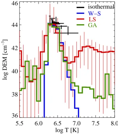
to 30 “best”, newly-generated DEMs hadχ2 values below 10. The evolution process was repeated 6 times, each time starting from a new random population. As a result we ob-tained 136 solutions withχ2<10. In Fig. 7 the green line presents the mean of these 136 solutions (χ2of the mean is 4.7). The errors were calculated as a standard deviation from the mean. The solution obtained with GA hasχ2less than those obtained with WS and LS methods.
The Withbroe-Sylwester (WS) method is iterative, multi-plicative algorithm relying on the maximum likelihood ap-proach. In our calculations we started from a constant value DEM approximation. For detailed descriptions of this method, see Withbroe (1975) and Sylwester et al. (1980). Us-ing the WS method we performed 200 simulations consistUs-ing of 3000 iterations each. The obtainedχ2were in the range from 5 to 25. The mean solution hasχ2=10 (see Fig. 7).
Least-squares (LS) method – this procedure calculates DEM based on a least-squares fit of the calculated fluxes to the observed ones. The method is described in more detail by Weber et al. (2004) and implemented as a xrt dem iterative routine in SolarSoft. The DEM function is evaluated from some spline points, which are directly manipulated by theχ2
fitting the routine. Using the LS method we performed 200 LS-simulations. The obtainedχ2were in the range from 20 to 30. The mean solution hasχ2=25.
440 450 460 470 480 X (arcsecs)
-170 -165 -160 -155 -150 -145 -140
Y (arcsecs)
Open/Al_mesh
440 450 460 470 480
X (arcsecs) -170
-165 -160 -155 -150 -145 -140
Y (arcsecs)
Be_thin/Open
440 450 460 470 480
X (arcsecs) -170
-165 -160 -155 -150 -145 -140
Y (arcsecs)
[image:6.595.52.547.64.176.2]Open/Al_thick
Fig. 6. Images of the loop observed in active region NOAA 09555 around 18:00 UT, taken in three different Hinode/XRT filters. Contours overplotted on an Al mesh filter image corresponds to 0.6 and 0.8 of the maximum flux of the loop.
5.5 6.0 6.5 7.0 7.5 8.0 log T [K]
36 38 40 42 44 46
log DEM [cm
−3 ]
W−S
LS
GA
isothermal
Fig. 7. The DEM distributions of the loop observed on 13 May 2007 obtained using the three analysed numerical methods and us-ing isothermal approximation with different filter pairs.
We have tested all three methods using a synthetic isother-mal model. The reconstructed width of the solutions allow us to estimate the temperature resolutions of the method. This resolution is low at the edges of the considered temperature range (5.5<logT<8) and increase in the temperatures where the response functions have their maxima (see Fig. 1), with best values of dlogT=0.5–0.6, 0.2–0.3 and 0.1–0.2 for the LS, WS and GA methods, respectively. DEM errors are sim-ilar for all three methods, and we show in Fig. 7 only error bars for LS, for readness and transparency.
The uncertainties are in fact very large at lower temper-atures (see Fig. 7), and for this reason all three methods give solutions lying within error limits of both other meth-ods. Thus one cannot evaluate precisely EM in these
temper-atures using Hinode/XRT data. However, it is well known that DEM has a minimum around logT≈5.5 for quiet Sun and active regions, and for this reason, each obtained solu-tion could be correct (Brosius et al., 1996; Schmelz et al., 2001).
There are also differences in DEM solutions obtained for high temperatures. The LS solution indicates the presence of a bigger amount of the plasma having the temperatures in the range (7.0<logT<7.3) than the WS and GA methods. The differences are larger than estimated errors. A possible explanation of these differences is that LS models depend on initial approximation of DEM (Weber et al., 2004). The LS method also has the lowest temperature resolution com-paring to WS and GA methods. The difference between all three methods should be extensively tested using XRT obser-vations.
Obtainedχ2are rather high. Considering the whole loop instead of one or two pixels, the relative errors of flux de-crease and thusχ2increase (being much above 1.0). On the other side, there are still large uncertainties in the fluxes mea-sured with an Al thick filter which strongly influence DEM in high temperatures. A largeχ2value can also be attributed to uncertainties in atomic data which contribute to the sponse functions and to a systematic error in background re-jection.
3 Discussion and conclusions
XRT telescope can detect coronal plasma of various temper-atures ranging from less than 1 MK up to more than 10 MK. By applying observations made with two or more filters one can analyze coronal temperature and emission measured along a line-of-sight.
[image:6.595.66.265.243.470.2]analysis of the distribution of emission measure should be used.
The DEM distributions obtained with the described meth-ods are presented in Fig. 7. All three methmeth-ods give the main peak of emission for logT=6.3. Observed differences be-tween results of the three methods lie more or less within the error limits (please note the logarithmic scale of DEM). This figure also presents a set of isothermal solutions obtained for different pairs of filters. Their values lie around the main peak of DEM obtained with numerical methods described before. Thus, we can conclude that all three methods give results similar to the two filters ratio method.
We can also conclude that described methods of the DEM calculation gave similar and comparable solutions. Addi-tionally, based on the shapes of the emission functions (see Fig. 1) we can expect much better conformity of the results obtained with the WS, LS and GA methods in a case of strong flares. We can state that the majority of the pairs of the
Hinode filters allows one to derive the temperature and
emis-sion measure in the isothermal plasma approximation using standard diagnostics based on the two filters ratio method. The temperatures evaluated with this method for two non-flaring active region plasmas were in the range from around 1.5 MK to about 5 MK.
Acknowledgements. Hinode is a Japanese mission developed and launched by ISAS/JAXA, with NAOJ as domestic partner and NASA and STFC (UK) as international partners. It is operated by these agencies in co-operation with ESA and NSC (Norway).
This paper was supported by the Polish Ministry of Science and Higher Education, grants N203 022 31/2991 and N203 015 32/1891.
Topical Editor R. Forsyth thanks two anonymous referees for their help in evaluating this paper.
References
Brosius, J. W, Davila, J. M., Thomas, R. J., and Monsignori-Fossi, B. C.: Solar EUV spectroscopy with serts: measurements of ac-tive and quiet Sun properties, ApJS, 106, 143–164, 1996. Charbonneau, P.: Genetic Algorithms in Astronomy and
Astro-physics, ApJS, 101, 309–334, 1995.
Cirtain, J. W., Del Zanna, G., DeLuca, E. E., Mason, H. E., Martens, P. C. H., and Schmelz, J. T.: Active Region Loops: Tempera-ture Measurements as a Function of Time from Joint TRACE and SOHO CDS Observations, ApJ, 655, 598–605, 2007. Craig, I. J. D. and Brown, J. C.: Fundamental limitations of X-ray
spectra as diagnostics of plasma temperature structure, A&A, 49, 239–250, 1976.
Golub, L., DeLuca, E., Austin, G., et al.: The X-Ray Telescope (XRT) for the Hinode Mission, Solar Phys., 243, 63–86, 2007. Golub, L. and Pasachoff, J. M.: The Solar Corona, Cambridge:
Cambridge Univ. Press, 101–104, 1997.
Guedel, M., Guinan E. F., Mewe, R., Kaastra, J. S., and Skinner, S. L.: A Determination of the Coronal Emission Measure Distribu-tion in the Young Solar Analog EK Draconis from ASCA/EUVE Spectra, ApJ, 479, 416–426, 1997.
Kaastra, J. S., Mewe, R., Liedahl, D. A., Singh, K. P., White, N. E., and Drake, S. A.: Emission measure analysis methods: the corona of AR Lacertae revisited, A&A, 314, 547–557, 1996. McIntosh, S. W., Charbonneau, P., and Brown, J. C.:
Precondi-tioning the Differential Emission Measure (Te) Inverse Problem, ApJ, 529, 1115–1130, 2000.
McTiernan, J. M., Fisher, G. H., and Li, P.: The Solar Flare Soft X-Ray Differential Emission Measure and the Neupert Effect at Different Temperatures, ApJ, 514, 472–483, 1999.
Pottasch, S.: On the Interpretation of the Solar Ultraviolet Emission Line Spectrum, Space Sci. Rev., 3, 816–855, 1964.
Reeves, K. K., Parenti, S., Reale, F., and Weber, M. A.: Methods of Analyzing Temperatures in Post-Flare Loops using the XRT on Hinode, AGU Fall Meeting 2007, SH51C-08, 2007.
Schmelz, J. T., Scopes, J., Cirtain J. W., Winter H. D., and Allen J. D.: Observational Constraints on Coronal Heating Models Us-ing Coronal Diagnostics Spectrometer and Soft X-Ray Telescope Data, ApJ, 556, 896–904, 2001.
Sylwester, J., Schrijver, J., and Mewe, R.: Multitemperature analy-sis of solar X-ray line emission, Solar Phys., 67, 285–309, 1980. Thomas, R. J., Starr, R., and Crannell, C. J.: Expressions to deter-mine temperatures and emission measures for solar X-ray events from GOES measurements, Solar Phys., 95, 323–329, 1985. Vaiana, G. S., Krieger, A. S., and Timothy, A. F.: Identification and
Analysis of Structures in the Corona from X-Ray Photography, Solar Phys., 32, 81–116, 1983.
Weber, M. A., DeLuca, E. E., Golub, L., and Sette, A. L.: Tem-perature diagnostics with multichannel imaging telescopes, IAU Symp., 223, 321–328, 2004.