of Highly Deformable Drops in a Viscous
Flow with Spontaneous Marangoni Effect
Wei Gu, Olga Lavrenteva, and Avinoam Nir
Department of Chemical Engineering, Technion, Haifa 32000, Israel
Abstract. We report on three dimensional boundary-integral code and on simulations of the motion of highly deformable drops in the presence of Marangoni effect. Our focus is on the case when the concentration gradients that cause the tangential stresses on the interfaces are not externally imposed but are induced spontaneously induced by the in-terfacial transfer of surfactants (spontaneous Marangoni effect). When drops move in viscous fluid under intensive external forcing, large de-formations, cusps formation and breakup of the drops are typical. The results of the simulation of an initially deformed single drop in gravity field and in linear flow are presented. Our simulations show that even weak Marangoni effect may drastically change the deformation pattern in critical situations.
1
Introduction
The main advantage of the boundary integral equations (BIE) methods is the reduction of the dimension of linear problems as their implementation involves values of the variables only on the interfaces. These methods are extensively used for simulations of complex multiphase flows. In particular, numerous studies of the interaction of deformable drops in buoyancy-driven motion in creeping flow were performed making use of BIE methods and revealed a rich variety of defor-mation patterns depending on the Bond number and the initial configuration of the system (see e.g. Manga and Stone [1], Zinchenkoet al[2] and the literature cited).
Most of the BIE simulation available in literature are devoted to multiphase problems with tangential stresses continuous across the interfaces that is typical for pure interfaces in isothermal fluids. In contrast to this, in processes accompa-nied with heat or mass transfer, surface tension that depends on temperature and concentration of surface-active substance is not constant. Surface tension gradi-ents result in tangential stresses that, in turn, induce the so-called Marangoni flow in the vicinity of the interfaces. This flow may substantially alter the flow pattern, e.g. cause migration of drops in the absence of body forces. From the mathematical point of view, the boundary integral equation modeling of such flows contains an additional term with a tangential stress jump, which provides additional difficulties in the course of numerical solutions.
J. Zhang, J.-H. He, and Y. Fu (Eds.): CIS 2004, LNCS 3314, pp. 93–98, 2004. c
The goal of the present work was to develop a 3D boundary-integral code for the accurate calculations of the evolution of highly deformable drops in the presence of tangential stress jump and to employ it for simulation of various critical and near critical regimes such as breakup, coalescence and cusp formation in order to study the influence of the Marangoni effect in these processes. Our focus is on the case when the concentration gradients that cause tangential stress jump on the interfaces are not externally imposed but are spontaneously induced by the interfacial transfer of surfactants (spontaneous Marangoni effect).
2
Formulation of the Problem
Consider a number of drops of radii ai, i = 1, ..., n moving in an immiscible viscous fluid submerged in an unbounded Newtonian fluid which has a uniform constant concentration of a weak surfactantC0 at infinity. The initial
concen-tration inside the drops,C1, is constant and different fromC0. A Robin type
boundary condition is assumed on the interfaces for the concentration in the outer fluid (see [3] for the detailed discussion of the applicability of this model of mass transfer). It is supposed further that the concentration does not affect any physical properties of the liquids in the bulk and at the interfaces except for the interfacial tension which depends linearly on concentration,σ=σ0+σc(C−C0),
where∂σ/∂C is constant and typically negative. We shall be interested in the case of small Reynolds and Peclet numbers, when the inertial and convective transport effects are negligible.
The following scaling is chosen:a1 for length,v0 =η−01|σc|C1/ke−C0| for
velocity,a1/v0 for time andv0η0/a1 for the pressure. Hereke is the phase
dis-tribution coefficient (the ratio of equilibrium concentration inside and outside the drops),η0 is the viscosity of the continuous fluid andρ0 is its density. The
governing dimensionless parameters of the problem are the Marangoni number, M a=|σc|/(a1g∆ρ), the capillary number,Ca=η0v0/σ0, the ratios of the
ma-terial properties of the fluids, λi =η2/η1 and ρi/ρ1, and the initial geometry
of the system. The motion inside and outside the droplets is governed by the steady Stokes equations and satisfy the conventional conditions on the interfaces, while the dimensionless concentrationc(t,x) = (C−C0)/|C1/ke−C0|, x∈Ω
is harmonic outside of droplets, vanishes at infinity and satisfies
∂c/∂n=Sh(c−1), x∈∂Ω, (1) where Ω denotes the domain occupied by the continuous phase and∂Ω is the boundary separating it from the drops.nis an outer unit normal to a correspond-ing droplet interface andSh is the Sherwood number. Following the classical potential theory the concentration problem is reduced to a boundary-integral equation
2πc(x) +
∂Ω
Sh |r| +
r·n(y) |r|3
c(y)dSy =Sh
∂Ω 1
|r|dSy, (2)
After the equation of concentration is solved, the values of concentration at each node are available to compute the jump of normal and tangential stress across the interface. The velocity on the interfaces, thus, can be determined solving another system of boundary integral equations
v(x) = 2 1 +λi
v∞(x) + n
k=1
(1−λk)
P V
∂Ωk
K(r) :v(y)n(y)dSy
−n k=1
∂Ωk
J(r)
H
1
Ca−c(y)
n(y)−φ(y)n(y)−M a∇sc(y)
dSy
, (3)
x∈∂Ωi i= 1, ..., n, whereP V denotes the principal value,His a mean curvature,∇s=∇−(∇·n)n
is a surface gradient andφ(y) is a dimensionless body force potential. The kernels for the single and double layer potentials here are, respectively
J(r) = 1 8π
I
|r|+ r r
|r|3
, and K(r) =−3 4π
r r r
|r|5. (4)
3
Numerical Scheme and Result Discussion
3.1 Surface Discretization and Numerical Integration
The discretization of the surface is performed by means of uniform triangulation. An icosahedron, whose 20 triangular faces are inscribed into a sphere, is used as a basis for further triangulation. Each face of icosahedron is further divided into four triangles by connecting the edge midpoints. These vertices created by dividing triangles are projected radially on the sphere. Therefore, an umbrella neighborhood of 5 or 6 surrounding nodes and triangular elements is formed around each node. This process is repeated as many times as necessary. The total numberN of triangular elements is determined by the mesh orderkof the simulation,N = 20·4k.
A least square method is employed to calculate the normal vector, mean curvature and concentration gradient on the curved surfaces. A local coordinate system is built on each node to make local parametrization of this and the nodes in its neighborhood that is used to fit a paraboloid with least square method. However, the normal vector is not known a priori, and it is solved by iterative process. The works of Zinchenkoet al[2, 4] provide the details of this procedure. The values of concentration and velocity on each node stand for the averaged values within the 1/3 of its umbrella neighborhood that is used in the course of the numerical integration.
vector tangential to the interface. The singular integral of the first type can be analytically approximated as
∆ 1 |r|dS=
2∆S b Log
a+b+c
a−b+c, (5)
where∆Sis the area of the triangle for integration, whilea,bandc denote the length of each side of the triangle. For the singular integral of the second type, an analytical approximation is derived taking advantage of coordinate trans-formation, which converts the 3D integration into 2D integration and reduces the integrand to the form |r|−3(r·a)R−1·r, where R−1 is the inverse trans-formation matrix. a in this integration denotes the tangential component of concentration gradient.
3.2 Mesh Propagation and Redistribution
Because of the strong tangential flow on the interface, the propagation of the nodes with calculated velocities would result in an irregular mesh. Thus, mesh redistribution should be carried out for the purpose of mesh stabilization. The effect of local curvature should be taken into account when the surface tension matters in the thermal capillary interfacial flows. A curvature spring model is developed for this purpose, in which the local curvature and the size of mesh are significant to the mesh distribution. The mechanism of our curvature spring model is described as fij = kijmlnij (no summation), with fij being a spring force between nodes i and j; kij = (Hi+Hj)/2 is the elastic coefficient; lij = |rij+∆tvij| is the length between each pair of nodes, in which rij = ri−rj
andvij =vi−vj. m is any positive number whilen must be an odd integer. The density of the mesh is dynamically adjusted according to the distribution of curvature and the uniformity of the mesh. On one hand, increasingmwill pull more grid points to the regions of high curvature; on the other hand, increasing nwill make the mesh as uniform as possible.
The criterion of a ”good” distribution of mesh nodes is that the spring force imposed on each node satisfies the force balance on the tangential plane, which could be expressed mathematically asTNj=1fijeij
= 0, whereT is the
tan-gential projection operator,eij is the unit vector of the spring force, and N is the number of springs sharing the marked nodei. For practical computations, an iterative algorithm is used to calculate the corrected tangential velocity. Our simulations revealed that higher values ofmandnrequire more iterations.
3.3 Results of Simulations
(b)
(a)
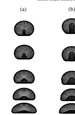
Fig. 1.Evolution of an initially oblate drop (λ= 5,Bo= 2,Sh= 1). (a) Buoyancy-driven motion. The drop will attain spherical shape. (b) Combined action of buoyancy and Marangoni effect. The drop will break up
con-centration and velocity are coupled when Marangoni effect is taken into account, otherwise, only the equation for the velocity is solved. Most calculations are per-formed for a mesh orderk= 3, where the drop has 1280 triangular elements on the interface. Test computations with a mesh order 4 have demonstrated that k= 3 is sufficient to acquire a reasonable numerical accuracy except for the cases with extremely high deformations. Runge-Kutta method is employed to make mesh advancement with a time step determined by CFL algorithm. For mesh redistribution, the combination ofm= 0.6 andn= 5 is found to be effective to stabilize the mesh and keep the mesh relative uniformity.
A sample result presented in figure 1 demonstrates the influence of the Marangoni effect on the motion and deformation of an initially oblate drop in a gravity field. Numerical simulation of the motion of an initially oblate drop with 1:4 aspect ratio with and without Marangoni effect is shown. The properties of the fluids are set toλ= 5,φ(y) =Bo(g·y), whereBo= 2 is the Bond number,
gis a unit vector in the direction of gravity andSh= 1.m= 1 and n= 5 are chosen for the mesh refinement. The shape of the drop could be compared to each other at the same time step 2.575, 4.155, 6.06, 8.72 and 11.75. The left and right sequences are calculated in the absence and in the presence of Marangoni effect, respectively. With the passage of time the drop driven solely by grav-ity attains a spherical shape, while under the combined action of gravgrav-ity and Marangoni effect, it breaks up. Thus, it is found that the tangential flow induced by concentration gradients influences the stability of the drop significantly.
Acknowledgement
The research was supported by ISF grant 74/01.
References
1. Manga, M., and Stone H. A.: Buoyancy-driven interaction between two deformable viscous drops. J. Fluid Mech.256(1993) 647-683.
2. Zinchenko, A., Rother M., and Davis, R.: Cusping, capture and breakup of interact-ing drops by a curvatureless boundary integral algorithm. J. Fluid Mech.391(1999) 249-293.
3. Golovin, A.A., Nir, A. and Pismen, L.P.: Spontaneous motion of two droplets caused by mass transfer. Ind. Eng. Chem. Res.34(1995) 3278-3288.
4. Zinchenko, A., Rother M., and Davis, R.: Phys. Fluids9, (1997) 1493-1511. 5. Berejnov, V., Lavrenteva O.M., and Nir, A.: Interaction of two deformable viscous
drops under external temperature gradient. J. Colloid Interface Sci. 242 (2001) 202-213.