On the interaction of four water-waves
Michael Stiassnie
a, Lev Shemer
b∗aFaculty of Civil and Environmental Engineering, Technion, Haifa 32000, Israel bFaculty of Engineering, Tel Aviv University, Tel Aviv 69978, Israel
Received 8 January 2004; received in revised form 21 June 2004; accepted 2 July 2004
Available online 11 September 2004
Abstract
The mathematical and statistical properties of the evolution of a system of four interacting surface gravity waves are investigated in detail. Any deterministic quartet of waves is shown to evolve recurrently, but the ensemble averages taken over many realizations with random initial conditions reach constant asymptotic values. The characteristic time-scale for which such asymptotic values are approached is extremely large when randomness is introduced through the initial phases. The characteristic time-scale becomes of an order comparable to that of the recurrence periods when beside the random initial phases, the initial amplitudes are taken to be Rayleigh-distributed. The ensemble-averaged results in the second case resemble, to a certain extent, those derived from the kinetic equation. © 2004 Elsevier B.V. All rights reserved.
Keywords: Water waves; Kinetic equation; Nonlinear interactions
1. Introduction
The dominance of quartet interactions in the nonlinear evolution of surface gravity waves was first established by Phillips [1]. The quartet interaction serves as the building brick in almost any model dealing with spectral evolution. The present work is based on Zakharov [2] equation for the temporal evolution of the complex amplitude spectrum. Zakharov’s equation is deterministic, i.e. no stochastic
∗Corresponding author. Tel.: +972 364 08128; fax: +972 364 07334. E-mail address: [email protected] (L. Shemer).
assumptions were made in the course of its derivation, and it is phase-resolving. Earlier, Hasselmann[3]
has derived an equation for the nonlinear evolution of the gravity-wave energy spectrum. In the derivation of Hasselmann’s equation certain assumptions about the stochastic properties of the system are necessary. These assumptions are often referred to by notions, such as: ‘nearly Gaussian process’, or/and ‘random phase approximation’. Details about application of these concepts to Zakharov’s equation in order to derive from it the Hasselmann equation can be found in a recent paper by Janssen[4]. The Hasselmann equation, sometimes called the kinetic equation, does not include information about the modal phases, and in this sense it is a phase-averaged equation.
Although the derivation of the kinetic equation does not explicitly require a large number of modes, it may be taken as implied through the assumption of ‘near Gaussianity’ which is expected to be maintained throughout the evolution, due to the central limit theorem.
The present work focuses on the evolution characteristics of an integrable system of four waves. The advantage in considering a four-wave system is that it allows a closed analytic solution. Such a solution can be used to examine the evolution parameters of a deterministic four-wave system for numerous initial conditions and for any instant, without the need for numerical integration of the governing equations. Moreover, by fixing some initial parameters and varying others, the statistics of the solution can be effectively studied, thus allowing direct estimates of the asymptotic behavior at long times.
A system of four ODEs is obtained from the Zakharov equation inSection 2(similar equations have been derived by the multiple scale method by[5]). Applying the technique of Bretherton[6], see also Shemer and Stiassnie[7], the detailed solution and its qualitative properties are given inSections 3–5, followed by a numerical example inSection 6. Stochastic aspects of the four-wave system evolution are raised in
Sections 7 and 8. InSection 7the initial phases are assumed to be random and uniformly distributed, while
inSection 8, Rayleigh distributed initial amplitudes are added. Comparison with solutions of Janssen’s
[4]version of the kinetic equation, for four modes, are given inSection 9. Discussion of the results is presented inSection 10.
2. Formulation
The nonlinear evolution of gravity-wave fields is dominated by the interactions of quartets[1]. The latter is reflected in the structure of Zakharov’s equation.
i∂B0
∂t
∞
=
−∞
V0,1,2,3B1∗B2B3δ0+1−2−3ei∆0,1,2,3tdk1dk2dk3 (2.1)
which has the quartets ‘built-in’, through the Delta-function and the frequency detuning
∆0,1,2,3 =ω0+ω1−ω2−ω3 (2.2)
The interaction coefficients V0,1,2,3= V(k0, k1, k2, k3) are given in Krasitskii[8]. The free-surface elevation is related to the generalized amplitude spectrum B(k,t) by
η= 1
2π
∞
−∞
k
2ω
1/2
where the frequencyωis given by the deep-water linear dispersion relation
ω2=g|k| (2.4)
In this paper we study the evolution of wave-fields, which consist of one quartet of free-waves only, so that
B(k, t)=Ba(t)δ(k−ka)+Bb(t)δ(k−kb)+Bc(t)δ(k−kc)+Bd(t)δ(k−kd) (2.5) where
ka+kb−kc−kd =0 (2.6)
Substituting (2.5) into (2.1) under the constraint (2.6) gives a system of four first-order nonlinear ordinary differential equations:
idBa
dt =(Ωa−ωa)Ba+2Vabcde
i∆a,b,c,dtB∗
bBcBd (2.7a)
idBb
dt =(Ωb−ωb)Bb+2Vabcde
i∆a,b,c,dtB∗
aBcBd (2.7b)
idBc
dt =(Ωc−ωc)Bc+2Vabcde
−i∆a,b,c,dtB∗
dBaBb (2.7c)
idBd
dt =(Ωd−ωd)Bd+2Vabcde
−i∆a,b,c,dtB∗
cBaBb (2.7d)
where the so-called ‘Stokes-corrected’ frequencies are:
Ωa=ωa+Vaaaa|Ba|2+2Vabab|Bb|2+2Vacac|Bc|2+2Vadad|Bd|2 (2.8a)
Ωb=ωb+2Vbaba|Ba|2+Vbbbb|Bb|2+2Vbcbc|Bc|2+2Vbdbd|Bd|2 (2.8b)
Ωc=ωc+2Vcaca|Ba|2+2Vcbcb|Bc|2+Vcccc|Bc|2+2Vcdcd|Bd|2 (2.8c)
Ωd =ωd+2Vdada|Ba|2+2Vdbdb|Bd|2+2Vdcdc|Bc|2+Vdddd|Bd|2 (2.8d)
3. Transition to a single unknown
Multiplying (2.7j) byBj∗, j = a, b, c, and d, and subtracting from the result its complex conjugate yields d
dt|Ba| 2= d
dt|Bb|
2= −d dt|Bc|
2= −d dt|Bd|
2 =
4VabcdIm{B∗aBb∗BcBdei∆a,b,c,dt} (3.1)
An auxiliary real function Z(t) is defined by
dZ
dt =Im{B
∗
aB∗bBcBdei∆a,b,c,dt}, Z(0)=0 (3.2) Substituting (3.2) into (3.1) and integrating gives
From (2.7) and (3.2) one can show that
d dtRe{B
∗
aBb∗BcBdei∆a,b,c,dt} = −ΩdZ
dt (3.4)
where
Ω=Ωa+Ωb−Ωc−Ωd ≡Ω0+Ω1Z (3.5)
andΩ0,Ω1are given by
Ω0=∆a,b,c,d+(Vaaaa+2Vabab−2Vacac−2Vadad)|βa|2+(2Vbaba+Vbbbb−2Vbcbc−2Vbdbd)|βb|2
+(2Vcaca+2Vcbcb−Vcccc−2Vcdcd)|βc|2+(2Vdada+2Vdbdb−2Vdcdc−Vdddd)|βd|2 (3.6a)
Ω1=4Vabcd{Vaaaa+Vbbbb+Vcccc+Vdddd+4Vabab−4Vacac−4Vadad−4Vbcbc−4Vbdbd
+4Vcdcd} (3.6b)
Integrating (3.4) from t = 0 gives
Re{B∗
aB∗bBcBdei∆a,b,c,dt} =Re{β∗aβb∗βcβd} − Z
0
ΩdZ (3.7)
From (3.2) and (3.7) we get
dZ dt
2
= |Ba|2|Bb|2|Bc|2|Bd|2−
Re{β∗
aβ∗bβcβd} −Ω0Z−
Ω1 2 Z
2
2
(3.8)
which is rewritten as
dZ dt
2
=P4(Z)= 4
=0
aZ4− (3.9)
where the coefficients of the forth-order polynomial P4(Z) are
a0= −0.25Ω21+256V 4
abcd (3.10a)
a1= −Ω0Ω1+64Vabcd3 (|βa|2+ |βb|2− |βc|2− |βd|2) (3.10b)
a2= −Ω20+Ω1|βaβbβcβd|cos(argβa+argβb−argβc−argβd)
+16Vabcd2 (|βaβb|2− |βaβc|2− |βaβd|2− |βbβc|2− |βbβd|2+ |βcβd|2) (3.10c)
a3=2Ω0|βaβbβcβd|cos(argβa+argβb−argβc−argβd)
−4Vabcd(|βaβbβc|2+ |βaβbβd|2− |βaβcβd|2− |βbβcβd|2) (3.10d)
4. Periodicity of amplitudes
The formal solution of (3.9) is
t= Z 0 dZ √
P4(Z) (4.1)
The actual details depend on the number and values of the real roots of the polynomial; and in principle, various scenarios may exist. However, for the examples that we study herein, we found that a0> 0 and 4 real roots Z4> Z3> 0 > Z2> Z1. For this case, we apply eq. (255.00) in Byrd and Friedman[9]and obtain from (4.1)
a1/2 0 t=γ
sn−1 (Z4−Z2)(Z3−Z) (Z3−Z2)(Z4−Z)
, κ
+sn−1 (δ, κ)
(4.2)
where sn is the Jacobian elliptic function with modulus
κ= (Z3−Z2)(Z4−Z1) (Z4−Z2)(Z3−Z1)
(4.3)
and
γ = √ 2
(Z4−Z2)(Z3−Z1)
(4.4a)
δ= Z3(Z4−Z2)
Z4(Z3−Z2)
(4.4b)
Inverting (4.2), we find
Z= Z4(Z3−Z2)sn2u−Z3(Z4−Z2) (Z3−Z2)sn2u−(Z4−Z2)
; u=sn−1(δ, κ)−a10/2t
γ (4.5)
Utilizing Eqs. (123.01) and (131.01) in Byrd and Friedman[9], we obtain
sn(u, κ)= δcn(a 1/2
0 t/γ) dn(a 1/2
0 t/γ)−s[(1−δ
2)(1−κ2δ2)]1/2sn(a1/2 0 t/γ) 1−(κδ)2sn2(a1/2
0 t/γ)
(4.6)
where
s=sgn(sinθ) (4.7a)
and
Note, that the amplitudes|Bj|, j = a, b, c, d in (3.3) depend on Z and thus are periodic, with period
T =2 Z3 Z2 dZ √ P4
= 2γ
a1/2 0
sn−1(1, κ)= 2γ
a1/2 0
K(κ) (4.8)
where K is the complete elliptic integral of first kind.
5. Evolution of phases
From (2.7) and (3.3) one can show that
argBa=argβa−2Vabcd t
0
β0−Ω0Z−(Ω1/2)Z2
|βa|2+4VabcdZ dt− t
0
(Ωa−ωa)dt (5.1a)
argBb=argβb−2Vabcd t
0
β0−Ω0Z−(Ω1/2)Z2
|βb|2+4VabcdZ dt− t
0
(Ωb−ωb)dt (5.1b)
argBb=argβc−2Vabcd t
0
β0−Ω0Z−(Ω1/2)Z2
|βc|2−4VabcdZ dt− t
0
(Ωc−ωc)dt (5.1c)
argBd =argβd−2Vabcd t
0
β0−Ω0Z−(Ω1/2)Z2
|βd|2−4VabcdZ dt− t
0
(Ωd−ωd)dt (5.1d)
where
β0= |βaβbβcβd|cosθ (5.2)
From (3.7) we obtain
Θ=argBa+argBb−argBc−argBd
=∆a,b,c,dt+cos−1 βo−ΩoZ−(Ω1/2)Z 2
[(4TabcdZ+|βa|2)(4T
abcdZ+ |βb|2)(−4TabcdZ+ |βc|2)(−4TabcdZ+ |βd|2)]1/2 (5.3)
For the free-surface elevationηto be periodic, the following condition must hold for each mode j = a, b,
c, d
argBj(T)−ωjT =argβj, (5.4)
Numerical results demonstrate that (5.4) does not hold. Thus, the recurrent four-wave system does not exhibit strict periodicity. However, from (5.3) it can be shown that
Θ(T)−∆a,b,c,dT =θ (5.5)
For exact resonance conditions, (5.5) demonstrates that the functionΘ(t) itself is periodic. An interesting consequence can be drawn from (5.5) for wave systems consisting of three different waves. This is the case treated by Shemer and Stiassnie[7]who considered degenerated quartets, where kb= ka, provided that kc is not collinear with ka(i.e. the problem is not one-dimensional). In these cases, the constraint (5.5), together with appropriate translation in the horizontal plane, enable to render two snapshots of the free-surface taken at t = 0 and t = T identical.
Thus, it seems that to a certain extent, one-dimensional deterministic solutions are “less organized” than their two-dimensional counterparts. Note that this relative “lack of organization” of the one-dimensional deterministic solutions can result in smoother ensemble averages when random initial conditions are added.
6. Example
Generally speaking, the input data consists of eight independent physical quantities: three wave-numbers ka, kb and kc, four amplitudes |βa|, |βb| |βc|, and |βd|, and one phase θ, see (4.7b). In our example, we are starting from a resonating quartet with: ka= (0.9806,−0.1961), kb= (0.9806, 01961), kc= (1.2903, 0.2747), kd= ka+ kb−kc= (0.6709,−0.2747); and allow variations in the components of
kc, kdin order to move away from exact resonance. The varied kcand kdare
kc =(1.2903−µ, 0.2747+µ); kd=(0.6709+µ, −0.2747−µ), (6.1)
for−0.15 <µ< 0.15.
Here and in the balance of the paper, we chose the case wherea= 0.2,b= 0.15,c= 0.08,d= 0.03. The initial amplitudes are given by
βj= πεj
|kj|
2g
ωj
1/2
, j=a, b, candd (6.2)
The initial phaseθis varied in the range (0, 2π).
The departure from exact resonance is indicated by a dimensionless scaled detuning parameter
∆=∆a,b,c,d/(ε2aωa) (6.3)
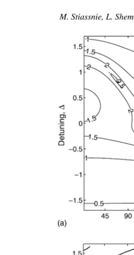
The dynamics of the system is captured by two dimensionless quantities:ρthe modulation range, andτ the modulation period. Since in all cases considered the auxiliary function Z varies in the interval Z2≤
Z≤Z3, and in light of (3.3), the modulation range is defined as
ρ= 4Vabcd(Z3−Z2)
Fig. 1. Isolines of (a) the modulation periodτ; (b) the modulation rangeρ.
The scaled modulation period is
τ= ε2aωaT
2π (6.5)
seeEq. (4.8).
Isolines ofτandρare shown inFig. 1a and b, respectively.
Note that the coordinate∆= 0 corresponds to the exact resonance conditions. The larger values of
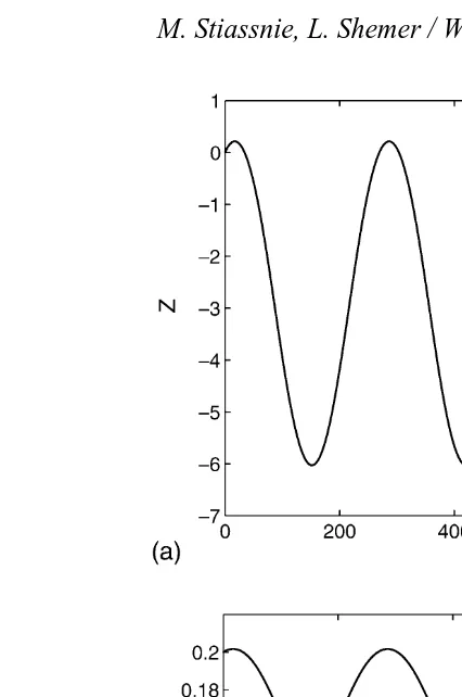
Fig. 2. Evolution of a near-resonant quartet; initial phases: arg(βa) =π/6; arg(βb) = 0; arg(βc) =−π/6; arg(βd) = 0. (a) auxiliary function Z; (b) wave amplitudes.
no means special, moreover, the extreme values forρandτare obtained for near-resonance, rather than for resonance conditions.
In the following Sections the discussion focuses on the influence of random initial conditions. In order to facilitate the assessment of the results in those Sections, it is instructive to compare them with the plots of deterministic results given inFig. 2.Fig. 2a and b give the evolution of Z and of the four amplitudes
kaaj, j = a, b, c, d, respectively. The dimensionless detuning parameter here is∆=−0.25 and the initial phaseθ=π/3. The time inFig. 2and elsewhere in this paper is rendered dimensionless by multiplication of the actual time byωa.
7. Random initial phase
Randomness is introduced into the problem through the initial conditions, using the notation
Here it is assumed that each of the argβj, (j = a, b, c, and d) is uniformly distributed over (0, 2π), but that the amplitudes|βj|are held fixed.
From (3.10) and (5.1), one can see that all|Bj(t)|depend solely on the combination θ, see (4.7b), whereas each arg Bj(t) depends also on its arg (βj), respectively.
The random initial phases guarantee the property of ‘statistical homogeneity’, defined as
βjβi∗ = |βj|2δi,j, (7.2)
where the brackets indicate an ensemble average andδi,jis the Kronecker delta. The ensemble average of any quantity Q is defined by
Q = 1
(2π)4
−π
−π
Q d(argβa)d(argβbd(argβc)d(argβd), (7.3)
From the structure of (5.1) and the definition (7.3) one can prove that Bj(t) maintain the property of ‘statistical homogeneity’, see (7.2), for all time. Moreover all first and third order moments:Bj,BjBiBk,
BjBi∗Bk; are zero.
The periodicity of any single realization of Z, and thus of all|Bj(t)|, has been shown inSection 4. In the Appendix we prove thatZ(t), which oscillates initially, settles down at large time to the asymptotic value
Z∞ = 1
2π
π
−π[Z1−
(Z4−Z2)(Z3−Z1) Z(β, κ)] dθ, (7.4)
whereβ= sin−1[(Z3–Z1)/(Z4–Z1)], and Z(β,κ) is the Zeta function of Jacobi.
The input data here is almost identical to that ofSection 6. The exception is that the near-resonant quartet to be discussed here and in sequel includes the following wave vectors: kaand kbas before, and
kc= (1.3060, 0.3102), yielding the dimensionless detuning parameter∆=−0.25, see Eq. (6.3).
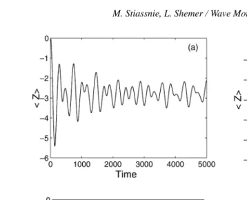
The evolution ofZin time is shown inFig. 3. The ensemble average was computed over Np= 2000 initial phasesθ. Two time intervals are shown, the first t∈(0, 5000) inFig. 3a and c, and the second t∈ (105, 1.05×10⁵) inFig. 3b and d. Note that the instant t = 5000 is reached after about 800 wave-periods. Adopting the notation tn = (2π/ωa)/εna, for the steepnessεunder consideration this is well within the t4 time-scale. ComparingFig. 3a and b for exact resonance, withFig. 3c and d for near resonance conditions, one can see that the former are somewhat more erratic, since the evolution of the latter is affected by the detuning frequency. The decay of the oscillations with time is evident for both quartets considered, albeit being extremely slow.
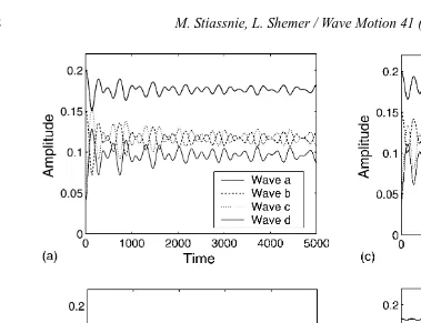
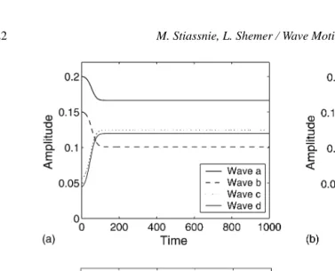
Fig. 4provides the evolution of the dimensionless averaged amplitudesAj, j = a, b, c, d, defined as
Aj = kπa ωj|Bj| 2
2g
(7.5)
Naturally, the behavior is very similar to that inFig. 3, due to the simple relations (3.3).
Fig. 3. Evolution of the auxiliary functionZ, averaged over 2000 initial phases: (a, b) for resonance conditions; (c, d) for near resonance conditions.
8. Numerical results for random initial amplitudes
As a second exercise we assume that (in addition to random initial phases), the initial amplitudes|βj| are random, and governed by the Rayleigh distribution, so that their pdf is
f(|βj|)= 2|βj|
|βj|2 exp
− |βj|2 |βj|2
, j=a, b, c, d (8.1)
The above assumption assures that allβjR,βjI, see Eq. (7.1), have a Gaussian distribution with zero mean and variance|βj|2/2. The question whether the Gaussianity of Bj(t) = BjR(t) + iBjI(t) is approximately maintained for all time, is an important issue in attempts to develop ‘phase-averaged’ equation, such as the kinetic equation. The values assigned to |βj|2 in (8.1) are the same as those assigned to|β
j|2 in
Sections 6 and 7.
In order to render the computations feasible, the number of random initial phases is reduced to
Np = 50. The number of realizations of the initial amplitudes for each one of the four modes was set to Na = 4–7. The overall number of realizations in the ensemble is NpN4
Fig. 4. Evolution of averaged wave-amplitudes (see Eq. (7.5), averaged over 2000 initial phases: (a, b) exact resonance; (c, d) near resonance conditions.
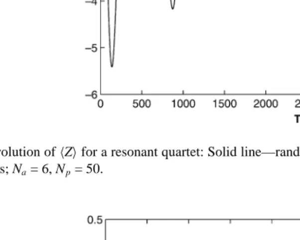
InFig. 5the evolution ofZwith random initial phases only is compared to the case where both initial
phases and amplitudes are random. The behavior is strikingly different, in the sense that for the latter case nothing interesting occurs for t > 750 = O(t3).
Computational results for two different numbers of initial amplitude realizations, Na = 4 and 7, are presented inFig. 6. The agreement between both graphs indicates that the Rayleigh distribution has been satisfactorily approximated.
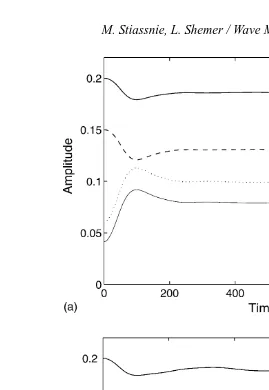
Fig. 7demonstrates the similarity between the evolution of the amplitudes for exact resonance
con-dition, to that for the near-resonant case. The similarity in the case of random initial amplitudes should be judged in light of the significant difference observed inFig. 4, where only random initial phases were considered.
Fig. 5. Evolution ofZfor a resonant quartet: Solid line—random phases only, Np= 2000; Dashed line—random amplitudes and phases; Na= 6, Np= 50.
[image:13.842.121.422.384.625.2]Fig. 7. Evolution of averaged wave amplitudes for Np= 50 and Na= 6 for (a) resonance conditions; (b) near-resonance conditions.
obtained also by Annekov and Shrira[10]who considered a finite number of clusters around wave modes that are in an exact resonance.
9. Comparison with the kinetic equation
Hasselmann[3]was the first to develop a ‘phase-averaged’ kinetic equation for C = <|B|2>. Recently, Janssen [4] has derived the following equation, which contains Hasselmann’s result as its long-time asymptotic limit:
∂C0
∂t =4
∞
−∞
V2
0,1,2,3{C2C3(C0+C1)−C0C1(C2+C3)}δ0+1−2−3
sin(∆0,1,2,3t)
∆0,1,2,3
dk1dk2dk3
Substituting
C(k, t)=Caδ(k−ka)+Cbδ(k−kb)+Ccδ(k−kc)+Cdδ(k−kc) (9.2)
into (9.1) yields
dCa dt =
dCb dt = −
dCc dt = −
dCd dt =8V
2
abcd{CcCd(Ca+Cb)−CaCb(Cc+Cd)}sin(∆∆a,b,c,dt) a,b,c,d (9.3)
The initial conditions are
Cj(0)=cj, j=a, b, c, d (9.4)
The system (9.3) can be reduced to a single equation, say for Ca:
dCa dt =8V
2
abcd{4C3a+3(db−dc−dd)C2a+2(dcdd−dbdc−dbdd)Ca2+dbdcdd}sin(∆∆a,b,c,dt) a,b,c,d
(9.5)
where
db =cb−ca; dc=cc+ca; dd =cd+ca; (9.6)
Denoting by c1, c2, c3 the roots of the third order polynomial in the curly brackets of (9.5), one can integrate (9.5) to obtain
C
a−c1
ca−c1
×
C
a−c2
ca−c2
b2/b1
×
C
a−c3
ca−c3
b2/b1
=exp
32Vabcd2
b1∆2
[1−cos(∆a,b,c,dt)]
(9.7)
where
b1 =
(c2–c3)
{c12(c2–c3)+c22(c3–c1)+c32(c1–c2)}
(9.8a)
b2 =
(c3–c1)
{c12(c2−c3)+c22(c3–c1)+c32(c1–c2)}
(9.8b)
b3 =
(c1–c2)
{c12(c2–c3)+c22(c3–c1)+c32(c1–c2)}
(9.8c)
For exact resonance conditions, one assumes that∆a,b,c,d→0, and (9.7) reduces to
Ca–c1
ca–c1
×
Ca–c2
ca–c2
b2/b1
×
Ca–c3
ca–c3
b2/b1
=exp
16V2 abcdt2
b1
(9.9)
Fig. 8. Evolution of averaged amplitudes: (a) kinetic equation, exact resonance; (b) kinetic equation, near-resonance; (c) and (d) as in (a) and (b), but for an ensemble average with Np= 50 and Na= 6.
Instead of considering implicit solutions (9.7) and (9.9), (9.5) can be integrated numerically using a Runge–Kutta method.
10. Discussion
The main purpose of this section is to shed light on the possible reasons for the significant quantitative differences between the results of the kinetic equation and those of the ensemble average approach, demonstrated inFig. 8. This requires, however, addressing first some aspects related to the derivation of the kinetic equation.
Taking the ensemble average of (3.1) gives
d dt|Ba|
2 = d dt|Bb|
2 = −d dt|Bc|
2 = −d dt|Bd|
2 =4V
abcdIm{Ba∗Bb∗BcBdei∆a,b,c,dt} (10.1)
−id
dt(B
∗
aB∗bBcBd)= {[Vaaaa+2Vabab−2Vacac−2Vadad]|Ba|2
+[2Vabab+Vbbbb−2Vbcbc−2Vbdbd]|Bb|2
+[2Vacac+2Vbcbc−Vcccc − 2Vcdcd]|Bc|2
+[2Vadad+2Vbdbd−2Vcdcd−Vdddd]|Bd|2}B∗aB∗bBcBd
+2Vabcd exp(−i∆a,b,c,dt){|Ba|2|Bc|2|Bd|2+ |Bb|2|Bc|2|Bd|2
− |Ba|2|Bb|2|Bc|2− |Ba|2|Bb|2|Bd|2} (10.2) In the course of derivation of the kinetic equation, an ensemble average of both sides of (10.2) is taken, and the following reduced version is adopted:
−id
dtB
∗
aB∗bBcBd =2Vabcd exp(−i∆a,b,c,dt){|Ba|2|Bc|2|Bd|2 + |Bb|2|Bc|2|Bd|2
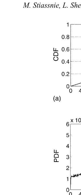
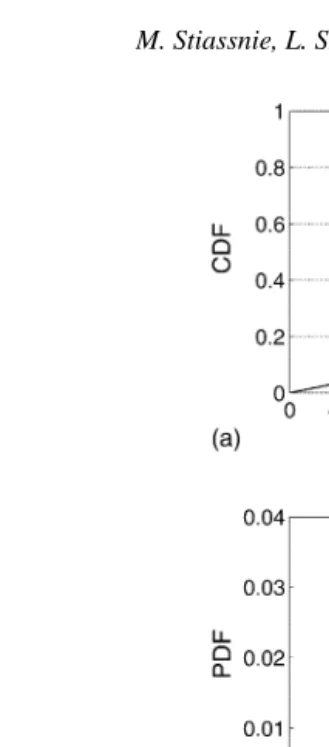
− |Ba|2|Bb|2|Bc|2 − |Ba|2|Bb|2|Bd|2} (10.3) See, for example the transition from (18) to (20) in Janssen[4], which makes use of the ‘nearly Gaussian process’ and ‘random phase’ approximations, expressing sixth order moments in terms of products of second order moments. In the case of an integrable system of four-waves, the phases, while initially random, develop a significant coherence in the course of evolution. This is evident from Fig. 9. The cumulative distribution function and the probability density function ofΘ(see Eq. (5.3)) at t = 1000 are presented in Fig. 9a and b, respectively. The ensemble average was calculated with Np = 100 and Na = 7. More dramatic results were obtained for constant initial amplitudes and Np= 50,000, seeFig. 10.
Fig. 10c shows the cumulative distribution function at an extreme coherent stage of the evolution process
that occurs around t = 100.
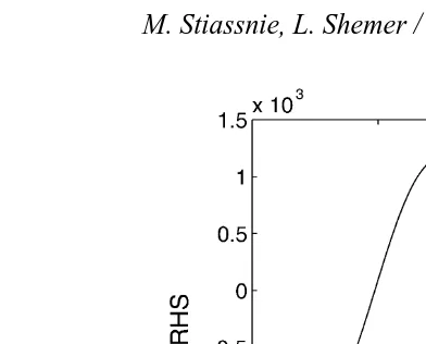
As a result of the behavior of the phases the RHS of (10.3) is a poor approximation of the ensemble average of the RHS of (10.2) for t > 20; this is seen from their plot inFig. 11.
It is our estimate that comparisons between results obtained by taking ensemble averages over many realizations of a deterministic system will compare more favorably with those from the kinetic equation, when the number of interacting modes in the system is increased. Indeed, Janssen[4]obtained a reasonably good agreement for 51 modes. The fact that we have obtained qualitatively similar behavior for four modes, was rather surprising to us.
Appendix A. on the behavior ofZ(t)at large t (proof of (7.4)).
The study of the deterministic problem yields the solution
Z(θ, t)=Z4−
Z4−Z3
1−(Z3−Z2/Z4−Z2)sn2u
; u=sn−1(δ, κ)−a10/2t
γ (A.1)
which is periodic in time, with period
T = 2γK(κ)
a1/2 0
Fig. 9. Resonant quartet, ensemble with Np= 100 and Na= 7: (a) cumulative distribution function ofΘat t = 1,000; (b) probability density function ofΘat t = 1000; (c) as in (a), but for t = 100.
and depends on the initial phase difference
θ=argβa+argβb–argβc–argβd (A.3)
In the stochastic approach we allow random values ofθ, with a uniform pdf in (−π,π]. The ensemble average is defined by
Z(t) = 1 2π
π
−π
Z(θ, t) dθ (A.4)
In this Appendix the asymptotic value ofZis calculated for large t:
Fig. 10. Resonant quartet, ensemble of 50,000 random initial phases: (a) cumulative distribution function ofΘat t = 1000; (b) probability density function ofΘat t = 1000; (c) as in (a), but for t = 100.
To this end, the periodicity of Z(θ, t) is utilized. Its Fourier expansion is:
Z(θ, t)=
∞
n=−∞
cn(θ) e2iπnt/T(θ) (A.6)
where
cn(θ)= T1 T
0
Fig. 11. A comparison of the ensemble average of the RHS of equation (10.2) (solid line), to the RHS of equation (10.3) (dashed line); Np= 50, Na= 6.
From (A.4) and (A.6) we obtain
Z(t) = 1 2π
∞
n=−∞
π
−π
cn(θ) e2iπnt/T(θ)dθ
(A.8)
Applying (A.5) to (A.8) yields
Z∞= 1
2π
∞
n=−∞
Cn, (A.9)
where
Cn =tlim→∞ π
−π
cn(θ) e2iπnt/T(θ)dθ (A.10)
The method of stationary phase guarantees that all Cn, for n=0, decay according to
Cn ∝t11/2 (A.11)
or faster, see p. 275 in Carrier et al.[13]. Thus, to the leading order, the contribution at large t comes from
C0, i.e.
Z∞= C0 2π +O(t
−1/2
) (A.12)
From (A.10) and (A.7)
C0= π
−π
where
c0= 1
T(θ) T
0
Z(θ, t) dt (A.14)
Substituting (A.1) into (A.14) gives
c0=Z4−
(Z4−Z3)
T
T
0
dt
1−α2sn2u (A.15)
where
α= Z3−Z2
Z4−Z2
(A.16)
Changing the integration variable in (A.15) from t to u, and utilizing (A.2):
c0(θ)=Z4−
Z4−Z3 2K
sn−1(δ,κ)
sn−1(δ,κ)−2 K
du
1−α2sn2u (A.17)
From Byrd and Friedman[9], p. 229, eq. (414.01) we obtain
c0(θ)=Z4−(Z4−Z3)
1+ αZ(β, κ) (1−α2)(κ2−α2)
=Z3−
(Z4−Z2)(Z3−Z1)Z(β, κ)
(A.18)
whereZ(β, κ) is the Zeta function of Jacobi and
β=sin−1
α
κ
=sin−1
Z3−Z1
Z4−Z1
, (A.19)
see Byrd and Friedman[9], p. 33.
Substituting (A.18) into (A.13), and (A.13) into (A.12) gives
Z∞= 21π
π
−π
Z3−
(Z4−Z2)(Z3−Z1)Z(β, κ)
dθ (A.20)
which is the final result, see Eq. (7.4).
References
[1] O.M. Phillips, On the dynamics of unsteady gravity waves of finite amplitude. Part 1, J. Fluid Mech. 9 (1960) 193–217. [2] V.E. Zakharov, Stability of periodic waves of finite amplitude on the surface of a deep fluid, J. Appl. Mech. Tech. Phys.
[3] K. Hasselmann, On the nonlinear energy transfer in a gravity-wave spectrum. Part 1. General theory, J. Fluid Mech. 12 (1962) 481–500.
[4] P.A.E.M. Janssen, Nonlinear four wave interactions and freak waves, J. Phys. Oceanogr. 33 (2003) 863–884. [5] D.J. Benney, Nonlinear gravity wave interaction, J. Fluid Mech. 14 (1962) 574–584.
[6] F.P. Bretherton, Resonant interaction between waves, J. Fluid Mech. 20 (1964) 457–480.
[7] L. Shemer, M. Stiassnie, in: Y. Toba, H. Mitsuyasu, Reidel F D. (Eds.), Initial Instability and Long-time Evolution of Stokes Waves, The Ocean Surface, Dodrecht, Holland, 1985, pp. 51–57.
[8] V.P. Krasitskii, On the reduced equations in the Hamiltonian theory of weakly nonlinear surface waves, J. Fluid Mech. 272 (1994) 1–20.
[9] P.F. Byrd, M.P. Friedman, Handbook of Elliptic Integrals for Engineers and Scientists, Springer-Verlag, 1971.
[10] S.Yu. Annenkov, V.I. Shrira, Direct numerical simulation of the statistical characteristics of waves ensembles, Doklady Phys. 49 (2004) 389–392.
[11] M. Onorato, A.R. Osborne, M. Serio, D. Resio, A. Pushkarev, V.E. Zakharov, C. Brandini, Freely decaying weak turbulence for sea surface gravity waves, Phys. Rev. Lett. 89 (2002) 144501–144601.
[12] K.B. Dysthe, K. Trulsen, H.E. Krogstad, H. Soquet-Juglard, Evolution of a narrow-band spectrum of random surface gravity waves, J. Fluid Mech. 478 (2003) 1–10.