Basic and extensible post-processing of eddy covariance flux data with REddyProc

https://doi.org/10.5194/bg-15-5015-2018 © Author(s) 2018. This work is distributed under the Creative Commons Attribution 4.0 License.

Basic and extensible post-processing of eddy covariance

flux data with REddyProc

Thomas Wutzler1, Antje Lucas-Moffat2,3, Mirco Migliavacca1, Jürgen Knauer1, Kerstin Sickel1, Ladislav Šigut4, Olaf Menzer5, and Markus Reichstein1

1_{Max Planck Institute for Biogeochemistry, Hans-Knöll-Straße 10, 07745 Jena, Germany}

2_{German Meteorological Service, Centre for Agrometeorological Research, Bundesallee 33, 38116 Braunschweig, Germany} 3_{Thuenen Institute of Climate-Smart Agriculture, Bundesallee 65, 38116 Braunschweig, Germany}

4_{Global Change Research Institute CAS, Bˇelidla 986/4a, 60300 Brno, Czech Republic} 5_{Department of Geography, University of California, Santa Barbara, CA 93106-4060, USA}

Correspondence:Thomas Wutzler ([email protected]) Received: 30 January 2018 – Discussion started: 12 February 2018

Revised: 6 August 2018 – Accepted: 7 August 2018 – Published: 23 August 2018

Abstract. With the eddy covariance (EC) technique, net fluxes of carbon dioxide (CO2) and other trace gases as well

as water and energy fluxes can be measured at the ecosys-tem level. These flux measurements are a main source for understanding biosphere–atmosphere interactions and feed-backs through cross-site analysis, model–data integration, and upscaling. The raw fluxes measured with the EC tech-nique require extensive and laborious data processing. While there are standard tools1 available in an open-source envi-ronment for processing high-frequency (10 or 20 Hz) data into half-hourly quality-checked fluxes, there is a need for more usable and extensible tools for the subsequent post-processing steps. We tackled this need by developing the REddyProcpackage in the cross-platform language R that provides standard CO2-focused post-processing routines for

reading (half-)hourly data from different formats, estimat-ing theu∗threshold, as well as gap-filling, flux-partitioning,

and visualizing the results. In addition to basic processing, the functions are extensible and allow easier integration in extended analysis than current tools. New features include cross-year processing and a better treatment of uncertainties. A comparison ofREddyProcroutines with other state-of-the-art tools resulted in no significant differences in monthly and annual fluxes across sites. Lower uncertainty estimates of both u∗ and resulting gap-filled fluxes by 50 % with the

1 http://fluxnet.fluxdata.org/2017/10/10/toolbox-a-rolling-list-of-softwarepackages-for-flux-related-data-processing/, last access: 17 August 2018

presented tool were achieved by an improved treatment of seasons during the bootstrap analysis. Higher estimates of uncertainty in daytime partitioning (about twice as high) re-sulted from a better accounting for the uncertainty in es-timates of temperature sensitivity of respiration. The pro-vided routines can be easily installed, configured, and used. Hence, the eddy covariance community will benefit from the REddyProcpackage, allowing easier integration of stan-dard post-processing with extended analysis.

1 Introduction

The availability of ecosystem-level observations of net ecosystem exchange (NEE) of carbon dioxide (CO2) and

other gases and latent heat (LE) and sensible heat (H) fluxes measured by the eddy covariance (EC) method (Aubi-net et al., 2000) greatly advanced ecosystem understand-ing at site to global scales (Baldocchi et al., 2017). The EC method provides half-hourly or hourly records of tur-bulent fluxes between an entire ecosystem and the atmo-sphere. These data are derived from high-frequency mea-surements (10 or 20 Hz) of wind speed and direction to-gether with measurements of air scalar characteristics such as CO2 and water vapor concentration, and temperature.

been consolidated in recent decades (Rebmann et al., 2012; Foken et al., 2012; Aubinet et al., 2012) and are available as open-source software2. Although measured continuously, the (half-)hourly EC data contain gaps due to instrument mal-functioning or records which are not representative of the ecosystem because of micrometeorological conditions under which the assumptions of the EC technique are not met (de-tails in e.g., Foken and Wichura, 1996; Foken et al., 2004, 2012; Göckede et al., 2004). Hence, (half-)hourly records are marked with different quality flags and need further extensive post-processing as described by Papale et al. (2006).

NEE records from periods with low friction velocity (u∗)

(Aubinet et al., 2012) need to be detected and filtered out to avoid systematic biases in nighttime NEE (Papale et al., 2006). The screened flux time series with gaps need to be filled (Reichstein et al., 2005a) using the available flux data and meteorological measurements. Additional information can be obtained from NEE thanks to flux-partitioning meth-ods that provide model estimates of gross primary production (GPP) and ecosystem respiration (Reco) (Reichstein et al.,

2005a). These gross fluxes are important to understand land– atmosphere interactions.

All these post-processing steps need to be performed rou-tinely for EC data. Hence, it is desirable to have automated and reproducible post-processing tools available that can be easily used, extended, and integrated into researchers’ own workflow. For this purpose we have compiled all rou-tines for the important CO2-focused post-processing steps

in theREddyProcpackage in the free and cross-platform R language. TheREddyProcpackage loads time series of quality-checked and storage-corrected fluxes and the basic set of meteorological variables and provides a software envi-ronment to performu∗threshold detection and filtering, gap

filling, and partitioning. Furthermore, a series of other func-tionalities like data import routines and data visualization are provided.

The objectives of the paper are to

1. provide a reference that describes the methodology of the processing used in theREddyProcpackage, and 2. show that the obtained results do not differ

sys-tematically from results obtained with standard post-processing implemented in the FLUXNET community (based on Papale et al., 2006; Reichstein et al., 2005a; Lasslop et al., 2010; Pastorello et al., 2017).

Appendix C explains abbreviations used. The first part of the paper (Sect. 2) describes the post-processing meth-ods. The second part (Sect. 3) presents the benchmarks of the REddyProc implementation with standard post-processing tools. It details differences in the

implementa-2 http://fluxnet.fluxdata.org/2017/10/10/toolbox-a-rolling-list-of-softwarepackages-for-flux-related-data-processing, last access: 17 August 2018

tions and possible consequences in obtained results and ag-gregated fluxes. Appendices A–B provide an overview of the package with the general design, an example of the post-processing, and links to resources that get readers started with post-processing their own data.

2 Methods of post-processing

The post-processing relies on half-hourly or hourly measure-ments of NEE and ancillary meteorological data ofu∗, global

radiation (Rg), air or soil temperature (Tair, Tsoil), and vapor pressure deficit (VPD). The fluxes should be quality-checked and, if applicable, storage-corrected before their use in the package.

The post-processing follows a specific workflow:

1. determination and filtering of periods with low turbulent mixing (u∗filtering),

2. replacement of missing data in the half-hourly/hourly records (gap filling), and

3. partitioning of NEE into the gross fluxes GPP and Reco

(flux partitioning).

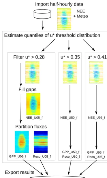
Usage of theREddyProcpackage follows this data post-processing workflow (Fig. 1). The following sections explain the steps in more detail.

2.1 u∗filtering

Determining periods with low turbulent mixing is a critical step in the EC data post-processing. Standard steady-state and integral turbulence characteristics tests in the initial pro-cessing exclude the most problematic records ofH, LE, and CO2fluxes (Foken and Wichura, 1996). However, it is well

known (summarized in Aubinet et al., 2012, chap. 5), that such a quality-checking strategy is not sufficient, especially in the case of CO2. Stable stratification that is present

of-ten during the nighttime dampens turbulence and leads to an underestimation of the nighttime NEE, i.e., the ecosys-tem respiration (van Gorsel et al., 2007). Massman and Lee (2002) proposed that unfavorable conditions could be de-tected by inspecting the relationship of nighttime NEE versus u∗. Within a similar time period and similar environmental

conditions respiration should not be dependent on theu∗. At

lowu∗ values, a negatively biased respiration is measured.

A heuristic class of methods, which is widely accepted, as-sumes that a threshold ofu∗can be established above which

nighttime fluxes are considered valid. Hence, theu∗

thresh-old is the minimum u∗ above which respiration reaches a

plateau (Fig. 2). This threshold is specific for each season of a site year. Uncertainties in theu∗threshold estimate

Import half-hourly data

Fill gaps

NEE + Meteo

Estimate quantiles of u* threshold distribution

Partition fluxes

NEE_U05_f NEE_U50_f NEE_U95_f

GPP_U05_f Reco_U05_f

GPP_U50_f Reco_U50_f

GPP_U95_f Reco_U95_f

u* > 0.35 u* > 0.41

Export results

Figure 1.The workflow starts with importing the half-hourly (or hourly) data, in this example the year 1998 of the DE-Tha site. Next, a probability distribution ofu∗threshold is estimated for each season. Gap filling and flux partitioning are performed for several quantiles of this distribution for an estimate of uncertainty. Finally the results are exported.

There are at least two methods of estimating theu∗

thresh-old: the moving point method (Reichstein et al., 2005c; Papale et al., 2006), which is currently more routinely used, and the breakpoint detection method (Barr et al., 2013). 2.1.1 Moving point method foru∗

The method of Papale et al. (2006) detects a plateau in the relationship of nighttime NEE versus u∗among all records

within a temperature subset by a moving point test of records binned into differentu∗bins.

The nighttime data (default: Rg<10 W m−2) are split into different times of year, here called seasons, to account for differing surface roughness. Then the data of each season are split into default six temperature subsets of equal size (ac-cording to quantiles). Within each temperature subset, data are split into 20 about equally sizedu∗bins. The default

mov-ing point method, calledForward2, determines the thresh-old based on theseu∗bins. It checks for each bin if the mean

NEE is higher than 0.95 times the mean of the following 10 bins. If this also holds true for the next bin, the meanu∗of

the bin is reported as the threshold. There are often subsets of data in which no clear threshold can be detected. Hence, there are quality criteria for whether the estimate of a given sub-set is used in subsequent aggregation. One quality criterion specifies that temperature and u∗ should not be correlated

within the temperature subset; another requires a minimum number of valid records within a subset. Next, theu∗

esti-mates for different temperature classes and seasons (details in Sect. 3.2.1) are aggregated to derive a robustu∗estimate.

Within one season, the median is taken across the estimates of different temperature subsets. Within 1 year, the maximum is taken across the associated seasons.

Records during the nighttime withu∗smaller than the

es-timated threshold are flagged as invalid and are replaced in the subsequent gap-filling processing step. In addition, each half hour after records withu∗smaller than the threshold is

flagged to be invalid.

2.1.2 Breakpoint detection method foru∗

Alternatively, breakpoint detection can be applied to the unbinned data, which avoids the sensitivity of the moving point method to the specifics of the binning schemes (Barr et al., 2013).REddyProcprovides this method by estimat-ing the breakpoint based on unbinned records within the sea-sons/temperature subsets using thesegmentedR-package (Muggeo, 2003, 2008). However,REddyProcdiffers from Barr et al. (2013) by keeping the same aggregating scheme of seasonal/temperature estimates to annual thresholds as with the moving point method.

2.1.3 Bootstrapping uncertainty of theu∗threshold Estimates of the u∗ threshold are often sensitive to the

specifics of the combination of methods and the data, e.g., the binning, minimum number of records within a season or temperature subset, and criteria in aggregation. Therefore, a bootstrap (resampling with replacement) is applied to gener-ate 200 artificial replicgener-ates of the dataset, and for each repli-cate the threshold is estimated (Efron and Tibshirani, 1986; Davison and Hinkley, 1997). The 5th, 50th, and 95th per-centile of the estimates are reported as a range of threshold estimates. The subsequent post-processing steps of gap fill-ing and partitionfill-ing are then repeated usfill-ing those different thresholds to propagate the uncertainty ofu∗threshold

esti-mation to derived quantities such as annual NEE, GPP, and Reco.

2.2 Gap-filling methods

After quality checks and u∗ filtering, the dataset of

half-hourly NEE fluxes may contain up to 50 % gaps (sometimes this fraction is even higher, depending on the site conditions). For the benchmark datasets used in this paper, the percent-age of gaps beforeu∗filtering was on average 32 % and after

0.2 0.4 0.6 0.8 −2

0 2 4 6 8

u* (ms−1₎

NEE (gC

m

−

2yr

−

1)

+ ++++++

+ + + ₊ +

++ + +

+ +

1998006 (01.06.98−31.08.98) (9.3−10.8°C)

u* threshold = 0.42

Figure 2.Concept of theu∗filter: nighttime NEE at lowu∗is biased towards lower NEE values compared to cases with higheru∗. Unbiased NEE should scatter around the same plateau because environmental conditions are similar. Theu∗threshold (dashed line), i.e., the value below which this bias is considered significant, is estimated by a moving point method onu∗bins (crosses) across half-hourly records (circles). The example uses a subset of data from DE-Tha.

estimates, respectively. Filling of gaps in half-hourly NEE data is necessary to obtain complete time series for the cal-culation of daily averages or balances such as monthly or seasonal sums. The following three gap-filling methods are implemented inREddyProc.

2.2.1 Look-up tables

In the look-up table (LUT) approach, the fluxes are binned by the meteorological conditions within a certain time window. Within the chosen time window and respective bin, each me-teorological variable deviates less than a fixed margin to en-sure similar meteorological conditions. The missing value of the flux is then calculated as the average value of the binned records and its uncertainty estimated from their standard de-viation.

The original LUT of Falge et al. (2001) consisted of fixed periods over a year, while inREddyProcthe meteorolog-ical conditions are sampled with a moving window around the gap to be filled.

2.2.2 Mean diurnal course

NEE fluxes have a mean diurnal course (MDC) that follows the course of the sun with only respiration during nighttime and a combination of respiration and photosynthesis during daytime. This autocorrelation of the fluxes is exploited by taking the average value at the same time of day within a moving time window of adjacent days (Falge et al., 2001). In REddyProcthe same time of day also includes the fluxes of the adjacent hour (±1 h).

Though the MDC method only showed a medium perfor-mance in the gap-filling comparison for net carbon fluxes by Moffat et al. (2007), it has the advantage that this approach can be used even if no meteorological information is avail-able.

2.2.3 Marginal distribution sampling

The so-called marginal distribution sampling (MDS) by Reichstein et al. (2005b) exploits the covariation of the fluxes with the meteorological variables and their temporal autocorrelation based on the two methods LUT and MDC described above.

The filling of each half-hourly NEE with the MDS algo-rithm depends on the availability of the meteorological data of Rg, Tair, and VPD. (1) If all three meteorological vari-ables are available, LUT will be used with default margins of 50 W m−2, 2.5◦C, and 5.0 hPa, respectively. (2) If Tair or VPD are missing, only the variable Rg will be used. (3) If no meteorology is available, the gaps are filled with MDC. Fol-lowing a specific sampling procedure, the MDS algorithm increases the number of days in the vicinity of the gap until there are enough data points (at least two) for gap filling. A more detailed description with a flow diagram is provided in the Supplement.

The MDS algorithm is optimized for carbon dioxide and water fluxes and can also be used to estimate the uncer-tainty of the half-hourly fluxes. In the comparison of gap-filling methods by Moffat et al. (2007), the MDS algorithm performed well for different artificial gap scenarios ranging from single half-hours to several days. Due to its flexibil-ity in dealing with missing meteorological input data and its fast and highly automated routines available as an online tool (BGC16, Sect. 3), the MDS gap-filling method has been widely used.

2.3 Flux-partitioning methods

The gross fluxes of GPP into the land system and Reco

out of the land system are the two opposing parts of NEE: NEE=Reco−GPP. Availability of GPP and Recois pivotal

ra-diation, temperature, and soil moisture) is important to in-terpret land–atmosphere interactions and to improve earth system models (Reichstein et al., 2012). Therefore several methods were developed to partition NEE into these two components (Reichstein et al., 2005c; Lasslop et al., 2010; Moffat, 2012; Wehr and Saleska, 2015; Desai et al., 2008; Stoy et al., 2006).

The two most widely used methods are the so-called night-time partitioning and daynight-time partitioning (Reichstein et al., 2012). The nighttime partitioning (Reichstein et al., 2005c) relies on the temperature response function of nighttime NEE fluxes that are representative of Reco. It assumes that this

re-lationship is also applicable to daytime data. The rere-lationship is then used to predict Recofrom measured temperature and

GPP is computed as a difference between Recoand NEE. This

method is currently the most widely used approach. Alterna-tively, the daytime partitioning (Lasslop et al., 2010) fits a model to observations of daytime NEE and global radiation, accounting for the effects of radiation and VPD on GPP as well as the effects of temperature on Reco.

2.3.1 Nighttime flux partitioning

The method of Reichstein et al. (2005c) estimates a tem-porally varying respiration–temperature relationship from nighttime data. First nighttime data are selected by a thresh-old of Rg<10 W m−2, which is congruent with the BGC on-line tool (BGC16, Sect. 3), but differs from the 20 W m−2 re-ported in Reichstein et al. (2005c). Additionally, nighttime data are constrained between computed sunset and sunrise.

Next, temperature sensitivity,E0, of the Lloyd and Taylor

(1994) relationship (Eq. 1) is estimated by fitting the model to successive 15-day periods of nighttime data, and the re-sultingE0series is aggregated to an annual estimate.

Reco(T )=RRefexp

E0

₁

TRef−T0

− 1

T−T0

, (1)

whereT0 is kept constant at−46.02◦C (Lloyd and Taylor,

1994) and where the reference temperature TRef is 15◦C,

which is congruent with the BGC online tool (BGC16, Sect. 3), but differs from the 10◦C reported in Reichstein et al. (2005c). For robustness each fit is repeated on a trimmed dataset excluding records with residuals outside the 5 %–95 % residual distribution. The annual aggregate is the mean across the three valid estimates with the lowest uncer-tainty in the fit. Single estimates ofE0are considered valid

if there were a minimum of six records, temperature ranged across at least 5◦C, and estimates were inside the range of 30 to 450 K.

Subsequently, the respiration at reference temperature, RRef, is re-estimated from nighttime data using the annualE0

temperature sensitivity estimate for 7-day windows shifted consecutively for 4 days. The estimated value is then as-signed to the central time point of the 4-day period and

linearly interpolated between periods. Hence, the obtained respiration–temperature relationship varies across time.

Finally, Recois estimated for both day- and nighttime from

the temporarily varying Reco–temperature relationship, and

daytime GPP is computed as Reco–NEE.

2.3.2 Daytime flux partitioning

The method of Lasslop et al. (2010) models NEE using the common rectangular hyperbolic light-response curve (LRC) (Falge et al., 2001):

NEE= αβRg αRg+β

+γ , (2)

whereα(µmol CO2J−1) is the canopy light utilization

effi-ciency and represents the initial slope of the light-response curve,β (µmol CO2m−2s−1) is the maximum CO2uptake

rate of the canopy at infinite Rg, andγ (µmol CO2m−2s−1)

is a term accounting for ecosystem respiration. The hyper-bolic light-response curve is modified to account for the temperature dependency of respiration after Gilmanov et al. (2003) by setting respirationγ to the Lloyd and Taylor res-piration model (Lloyd and Taylor, 1994) (Eq. 1). Further, the constant parameterβ in Eq. (2) is replaced by an exponen-tial decreasing function (Körner, 1995) at higher VPD values (Eq. 3).

β=

(

β0exp [−k(VPD−VPD0)] if VPD>10 hPa β0otherwise

, (3)

where the VPD0threshold is 10 hPa in accordance with

ear-lier findings at the leaf level (Körner, 1995), ignoring poten-tial vegetation specific differences.

ParameterT0in Eq. (1) was fixed as in the nighttime

par-titioning (Sect. 2.3.1). ParameterTRefwas fixed in each

win-dow to the median temperature within the winwin-dow. The other parameters (E0, RRef, α, β0, k) of the model are estimated by

the following steps. (1) A time-varying temperature sensitiv-ityE0is estimated from nighttime data for a window shifted

by 2 days. (2) TheE0 estimates are smoothed across

suc-cessive windows by fitting a Gaussian process (Rasmussen and Williams, 2006; Menzer et al., 2013) using themlegp R-package that also estimates uncertainty of the smoothed E0. Next, a prior respiration,RRef, for reference temperature TRef=15◦C is re-estimated from nighttime data for each

window with smoothedE0. (3) Parameters of the rectangular

hyperbolic light-response curve (RRef,α,β0,k) are fitted

us-ing only daytime data and the previously determined temper-ature sensitivity (E0) for each window. (4) Finally, for each

NEE record, GPP and Recoare estimated with the

Supplement reports necessary technical details about these steps.

Note, that contrary to the nighttime-based flux partition-ing, both GPP and Recoare model predictions and do not add

up exactly to observed NEE.

3 BenchmarkingREddyProc post-processing steps The post-processing steps’ implementations of REddyProc were benchmarked with the post-processing tools widely used in the FLUXNET processing. Specifically, REddyProc(version 0.8.1)u∗-filtering results were

com-pared with results by a C implementation from Dario Papale (Papale et al., 2006), referred to here as DP06. Results of REddyProc(version 1.1.3) gap filling and flux partitioning were compared with results obtained by the 2016 version web-based tool provided by the Max Planck Institute for Biogeochemistry, Jena, best described in Reichstein et al. (2005a). The tool was accessed in 2016 (29 July 2016) and is hereafter referred to as BGC16. Here, annually and monthly aggregated values refer to the mean across all valid values in a month or a year, which can differ from real annual or monthly budgets in the presence of large gaps. The first section describes the dataset used for benchmarking for each processing step implemented in the package. Within each of the following sections for the processing steps, subsections describe differences in the code, report the results of benchmarking, and discuss them. The Supplement, additionally, provides more detailed results and statistics. 3.1 Dataset used for benchmarking

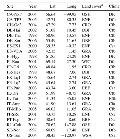
Data of 25 sites of the LaThuile FLUXNET dataset3, which have an open data policy, were used for benchmarking. The sites are located in different climate zones and belong to a variety of plant functional types (Table 1) to guarantee test-ing of different conditions (i.e., presence of snow, manage-ment such as cuts and crop rotation, sites disturbed) and ecosystem types (e.g., deciduous versus evergreen forests, grasslands and croplands). For each site the following vari-ables were used: NEE already filtered for quality flags (Fo-ken and Wichura, 1996), despiked and u∗-filtered (Papale

et al., 2006), random error of NEE computed as described by Reichstein et al. (2005a), Tair, Tsoil, Rg, and VPD. More-over, NEE time series before the u∗ filtering and the u∗

data were downloaded from AMERIFLUX and the European Flux Database to test the u∗ threshold estimation. Finally,

time series of gap-filled NEE (NEEf) and GPP partitioned

with the nighttime-based method (GPPNT) (Reichstein et al.,

2005a) were downloaded from the LaThuile dataset, while GPP partitioned with the daytime method (GPPDT) was

com-puted with BGC16.

3_{http://www.fluxdata.org, last access: 17 August 2018}

Table 1. Description of sites and times used for benchmarking

REddyProc.

Site Year Lat Long Land covera Climateb

CA-NS7 2004 56.64 −99.95 OSH Dfc

CA-TP3 2005 42.71 −80.35 ENF Dfb

CH-Oe2 2004 47.29 7.73 CRO Cfb

DE-Hai 2002 51.08 10.45 DBF Cfb

DE-Tha 1998 50.96 13.57 ENF Cfb

DK-Sor 2006 55.49 11.65 DBF Cfb

ES-ES1 2000 39.35 −0.32 ENF Csa

ES-VDA 2005 42.15 1.45 GRA Cfb

FI-Hyy 1998 61.85 24.29 ENF Dfc

FI-Kaa 2001 69.14 27.30 WET Dfc

FR-Gri 2006 48.84 1.95 CRO Cfb

FR-Hes 1998 48.67 7.06 DBF Cfb

FR-Lq1 2006 45.64 2.74 GRA Cfb

FR-Lq2 2006 45.64 2.74 GRA Cfb

FR-Pue 2003 43.74 3.60 EBF Csa

IE-Dri 2004 51.99 −8.75 GRA Cfb

IL-Yat 2005 31.34 35.05 ENF BSh

IT-Amp 2004 41.90 13.61 GRA Cfa

IT-MBo 2005 46.02 11.05 GRA Cfb

IT-SRo 2001 43.73 10.28 ENF Csa

PT-Esp 2004 38.64 −8.60 EBF Csa

RU-Cok 2004 70.62 147.88 OSH Dfc

SE-Nor 1997 60.09 17.48 ENF Dfb

US-Ton 2004 38.43 −120.97 WSA Csa

VU-Coc 2002 −15.44 167.19 EBF Af

a_{Abbreviations for land cover type from International Geosphere-Biosphere Programme}

(IGBP) classification: CRO: cropland, DBF: deciduous broadleaf forest, EBF: evergreen broadleaf forest, ENF: evergreen needleleaf forest, GRA: grassland, OSH: open shrubland,

WET: permanent wetland, WSA: woody savanna.b_{Abbreviations for climate from}

Köppen–Geiger classification: Af: equatorial, rainforest; BSh: hot arid steppe; Cfa: humid, warm temperate, hot summer; Cfb: humid, warm temperate, warm summer; Csa: summer dry, warm temperate, hot summer; Dfb: cold, humid, warm summer; Dfc: cold, humid, cold summer.

3.2 u∗filtering: benchmarking with DP06

Estimation of theu∗threshold byREddyProcusing the

de-fault moving point method (Sect. 2.1.1) was benchmarked to estimation based on Papale’s DP06 C implementation (Papale et al., 2006). The benchmark applied a bootstrap sample of size 60 and recorded lower, median, and upper quantiles of 10 %, 50 %, and 90 % instead of the default 5 % and 95 % based on a larger sample size to save computing time.

The different estimates of theu∗threshold have potential

consequences for the inferred fluxes. To explore these conse-quences, we used the different resulting thresholds to mark gaps, gap-fill the data, and compute the annual NEE based on the gap-filled time series. NEE uncertainty was estimated by the difference between NEE based on the lower quantile u∗and NEE based on the upper quantileu∗estimate.

3.2.1 Differences in code

op-tion, which is also employed by DP06, records of December are associated with the same season as January and Febru-ary of the same year. With the default continuous classi-fication, seasons start the same as in DP06 by default in March, June, September, and December. However, Decem-ber is treated in the same season as January and February of thenextyear to avoid discontinuities at year boundaries. The annualu∗ threshold is then applied according to those

con-tinuous seasons spanning year boundaries. For example, the processing of 2014 data would by default use data from win-ter 2014 (starting in December 2013) to autumn 2014 (end-ing in November 2014).REddyProcalso allows more flex-ibility with the user-specifiedclassification into seasons as explained below.

There are further slight differences between REddyProc and DP06. Both methods bin in a way such that the number of records in each bin is similar. If there are numerically equal u∗ values, they are sorted into

the same bin, resulting in bins with unequal record numbers. In DP06 sometimes no records are sorted into the subsequent bins, hampering the moving point detection. Conversely, the binning withREddyProcensures that there are a minimum number of records in all bins. This often results in fewer bins. Moreover, differing from DP06,REddyProcemploys several more quality criteria. First, when comparing the threshold bin to NEE in the following bins, it makes sure that there are least three bins to infer a plateau in NEE. Next, when aggregating the thresholds of different temperature classes to season, it ensures that a threshold was found in at least 20 % of the temperature classes. For those seasons during which no threshold could be determined, the annual estimate is used. When there are too few records within a year, a single season comprising all records is used for threshold estimation.

Differently to DP06, REddyProc only resamples data within seasons instead of across the entire year during the bootstrap, in order to protect periods of a similar u∗–NEE

relationship and to avoid seasonal biases in resampling. 3.2.2 Benchmark results

The general relationship in the estimation of theu∗threshold

was retained between the two methods (Fig. 3), although in-dividual threshold estimates differed. The exceptionally high threshold value of >0.6 m s−1 for site FR-Pue was very probably an overestimate by DP06. However, one has to re-member that each estimate has a high uncertainty, and the differences between the two methods were in the range of this uncertainty (Supplement). The estimate of the uncer-tainty of theu∗thresholds withREddyProcwas, however,

only half of the uncertainty range estimated by DP06 (Sup-plement). This increased precision was mainly due to the modified bootstrapping scheme, which respects the u∗

sea-sons.

FR−pue

y=0.0634+0.885x R2=0.53

0.0 0.2 0.4 0.6

0.1 0.2 0.3 0.4 0.5

u* thresholdREddyProc (m s−1)

u* threshold

D

P

06

(

m

s

−

1 )

Figure 3.u∗thresholds derived using different methods deviate for single sites. The relationship across site years is retained as indi-cated by a regression (solid line with shaded uncertainty bound) close to the 1 : 1 line (dashed).

y= −3.55+1.02x R2=0.99 −600

−300 0 300

−750 −500 −250 0 250

NEEREddyProc (gC m−2 yr−1)

N

E

ED

P

06

(

gC

m

−

2 yr

−

1 )

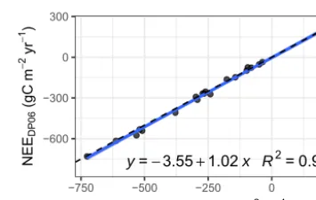
Figure 4.Strong correspondence in NEE based on theu∗ thresh-old estimated byREddyProcand NEE based on theu∗threshold estimated by DP06 across site years.

When propagating the differences inu∗ to differences in

annual NEE, there was no bias and decreased scatter across sites between all the methods (Fig. 4), despite the differences inu∗threshold. The absolute differences in annual NEE

be-tween the methods were small (mostly<20 gC m−2yr−1), and mostly lower than half of the uncertainty range estimated from the bootstrap (Supplement).REddyProc estimates u∗ thresholds with roughly double the precision compared

to DP06, due to its protecting of seasons during bootstrap (Supplement).

3.2.3 Discussion ofu∗threshold estimation

The agreement between NEE based on u∗ estimates of

REddyProc moving point implementation and current FLUXNET standard post-processing (DP06) (Fig. 4) indi-cates that the sensitivity of NEE to theu∗threshold estimate

in the inferred ranges is low, which also explains the large uncertainty of theu∗threshold estimate. One reason for the

missing effect could be site selection of this study without many sites affected by advection, which show limited sat-uration of the NEE–u∗dependence. Since in such cases the

of both DP06 and REddyProcare appropriate due to the negligible effect on NEE sums. The agreement implies that both methods can be interchanged in studies that are based on aggregated values, such as annual carbon budgets or for upscaling, without the need to reprocess data.

However, the increase in estimated precision, i.e., lower standard deviation, of theu∗threshold estimate also yields

an increase in estimated precision of the annual NEE by 50 % (Supplement). This will lead to improved accuracy and usability of EC measurements and any downstream, post-processed data products in model–data integration studies.

While the default seasons and their aggregation are in line with previous approaches,REddyProcallows site-specific knowledge to be used to derive better threshold estimates. For example, if there is a disturbance such as harvest, the u∗ threshold is expected to change and a different

thresh-old should be applied for filtering before and after the dis-turbance. In this case the user can define a season change at the harvest date and use season-specific threshold estimates instead of the annually aggregated estimate (Sect. B7 in Ap-pendix B).

3.3 Gap filling: benchmark with BGC16

The gap-filling implementation ofREddyProcwas bench-marked with the BGC online tool (BGC16, Sect. 3), which used pvWave code developed by Reichstein et al. (2005c). 3.3.1 Differences in code

Compared to the BGC16, the new implementation of the MDS algorithm in REddyProc was not limited to single years, but it filled the gaps with a window moving continu-ously over all years in the input data. This had the advantage of smoother gap filling over the end of the year, and this will especially be of interest for sites in which vegetation is not dormant during this time. This new feature led to different, probably more realistic gap-filled NEE values at the begin-ning and end of the year.

There were also slight differences in the sequence of win-dow sizes betweenREddyProcand BGC16. For MDC, the window size with BGC16 had a few more intermediate day steps than REddyProc, which affected longer gaps with missing meteorology. The default meteorological variables and margins for LUT (see Sect. 4.2.2 above) were the same in both implementations.

WhileREddyProcrestricts gap filling to the interpola-tion of gaps, BGC16 also restricted missing records in peri-ods without measurements.

3.3.2 Benchmark results and discussion for gap filling In the benchmark,REddyProcgap filling was run using the same measured NEE as input that passed the QA/QC routines andu∗ filtering. The annually aggregated values comprised

both filled gaps and originally valid records.

−20 −10 0 10

−20 −10 0 10 NEEREddyProc (µ molCO2m−2s−1)

NEE

B

G

C

16

(

µ

mol

CO

2

m

−

2s

−

1) Quality flag

1 2 3

RU−Cok

y = 0.973 x R2 = 0.99

−750 −500 −250 0

−750 −500 −250 0 NEEREddyProc (gCm−2yr−1)

N

E

EBG

C

16

(

gC

m

−

2yr

−

1)

(a)

(b)

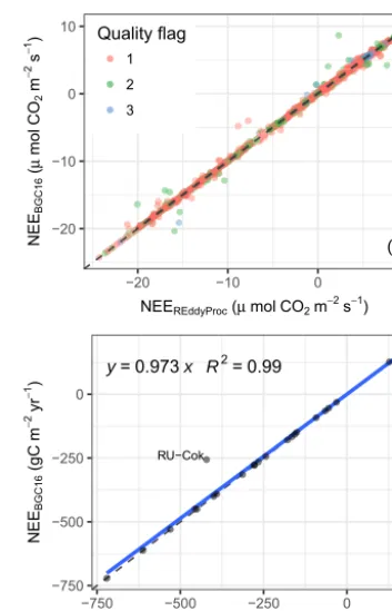
Figure 5.Predictions of NEE by REddyProcafter gap filling agree with BGC16 both at half-hourly values(a), shown for the DE-Tha 1998 case, and annual means across sites(b). Larger qual-ity flags are associated with larger window sizes.

REddyProcgap-filling results agreed with the results of BGC16. A few discrepancies at a half-hourly timescale were found mostly during longer gaps due to the usage of fewer window sizes, as shown for the DE-Tha case (Fig. 5a). At an annually aggregated timescale, the agreement between meth-ods was strong (R2=0.99) (Fig. 5b). The outlier of site RU-Cok is due to the availability of only a few months of data for the whole year. WhileREddyProcfilled gaps in the time period with available data, BGC16 extrapolated into the time before and after this period. The seasonal cycle was well re-produced at each site (Supplement).

The good agreement between NEE based on gap filling by REddyProcand gap filling by BGC16 (Fig. 5) implies that both gap-filling tools can be used interchangeably without the need to reprocess data.

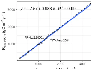
FR−Lq2.2006

IT−Amp.2004 y = −7.57+0.983 x R2 = 0.99

1000 2000 3000

1000 2000 3000 REcoREddyProc (gCm−2yr−1)

RE

co

B

G

C

16

(

gC

m

−

2yr

−

1)

Figure 6.Predictions of annually aggregated ecosystem respiration, Reco, fromREddyProcnighttime partitioning agree with the pre-dictions by BGC16.

3.4.1 Differences in code

The main features of the REddyProcimplementation of the nighttime-based partitioning algorithm were very simi-lar to BGC16, using a reference temperature of 15◦C and trimming the estimates of temperature sensitivityE0before

aggregating them (Sect. 2.3.1). REddyProcdiffered from BGC16 in computing the potential radiation that is used in subsetting the nighttime data to deriveE0and RRef

(Reich-stein et al., 2005c). WhileREddyProcused the exact solar time for the calculation of the potential radiation, where the sun culminates exactly at noon, BGC16 used the local win-ter time, which differs from the solar time depending on the location within the time zone.

3.4.2 Benchmark results and discussion for nighttime flux partitioning

Annual aggregated values of Recopredicted byREddyProc

were in very good agreement (R2=0.99; slope ≈1) with BGC16 as shown in Fig. 6 and in the Supplement.

In order to evaluate the effects of the differences intro-duced in the code described above, we also computed Reco

by prescribing eitherE0, or a selection of nighttime data, or

both from BGC16 output in REddyProc. Results are re-ported in the Supplement and showed that the most impor-tant factor affecting the Reco computed with REddyProc

was the different selection of nighttime data, though the dif-ferences were almost negligible at an annual timescale.

The two implementations agreed very well for most sites at an annual timescale. Because of no systematic deviations across sites, the spatial upscaling of fluxes should not be af-fected byREddyProcimplementation. However, for some sites, such as IT-Amp, the relative errors that are quite large indicate problems related to the selection of nighttime data and problems due to large gaps in the dataset.

3.5 Daytime flux partitioning: benchmark with BGC16 The daytime flux partitioning was benchmarked with results of the BGC online tool (BGC16, Sect. 3), which is based on pvWave code developed by Lasslop et al. (2010) and used in the processing of the 2015 FLUXNET release (Pastorello et al., 2017).

3.5.1 Differences in code

BGC16 differed fromREddyProc(Sect. 2.3.2), mainly in aspects of separation of nighttime data, estimation of temper-ature sensitivity from nighttime data, uncertainty estimation, treatment of missing values, and optimization library code.

While for separating nighttime dataREddyProcused the exact solar time, where the sun culminates exactly at noon, BGC16 used the local winter time.

For the estimation of temperature sensitivity E0 from

nighttime data, BGC16 used a reference temperature of 15◦C, instead of the median temperature inside the window. Hence, it estimated stronger correlations between parameters for windows with a different temperature range. Moreover, it omitted smoothing of the estimatedE0across time, often

leading to large fluctuations of theE0estimates across a few

days (Supplement), larger estimates of its uncertainty, and differences in subsequent estimation of LRC parameters.

For uncertainty estimation, BGC16 relied on the curvature of the LRC fit’s optimum instead of a bootstrap procedure. Hence, it could not take into account the uncertainty ofE0

estimated from nighttime data before the daytime LRC fit. Moreover, during interpolation of fluxes based on previous and subsequent valid estimates, the distance weights differed. WhileREddyProcassigned the estimates to the time of the mean of valid record in a window, BGC16 assigned it to the start of the third day, also if there were only valid data for the first day in the window.

For weighting the records in the LRC fit, BGC16 used the raw estimated NEE uncertainty of each record. It did not check for high leverage of spurious low NEE uncer-tainty estimates. Its estimates, therefore, were in some win-dows very strongly influenced by a few records, and failed if a NEE uncertainty estimate of zero was provided. More-over, when there were missing values or values below zero in a given NEE uncertainty, it set all uncertainty to 1, while REddyProcfilled the gaps by setting the missing uncer-tainty to the maximum of 20 % of respective NEE but at least 0.7 µmol CO2m−2s−1.

y=2.89+0.979x R2=0.98

RU−Cok

1000 2000 3000

1000 2000 3000 GPPREddyProc_Default (gCm−2yr−1)

GPP

BGC16

(

gC

m

−

2yr

−

1)

Figure 7. Prediction of annually aggregated GPP from

REddyProc daytime partitioning agree with BGC16 across sites.

For compatibility with BGC16, the above code differences can be disabled in REddyProc. But differences in opti-mization library code and specifically the conditions of non-convergence on scattered data could not be eliminated, which led to differences in results as shown in the following section. 3.5.2 Benchmark results for daytime partitioning Annually GPP predictions of both implementations showed no significant bias across the test sites (Fig. 7), although there was some scatter among individual predictions. Sim-ilar scatter was observed when comparing the predictions of the defaultREddyProcoptions to the predictions with com-patibility options. Most of the differences were caused by decreasing the unreasonable high influence of NEE records with small NEE uncertainty (Supplement).

The largest differences in aggregated fluxes between im-plementations were due to the extrapolation of fitted pa-rameters to periods where no parameter fits were obtained. In many of these cases, there were fits at the boundaries of these periods, whose validity was questionable. Whether these fits passed the quality check or not had a large in-fluence on the extrapolation and hence on the aggregated values. For example, at RU-Cok parameter estimates for valid periods agreed between implementations. However, no valid parameters could be obtained for winter months. While REddyProcreported missing values, BGC16 also reported GPP values based on summer parameterizations for periods further away from summer, which in turn led to higher annual GPP estimates.

Uncertainty estimates of gross fluxes approximately dou-bled with REddyProc due to the accounting for uncer-tainty in temperature sensitivity estimates from nighttime data (Supplement).

3.5.3 Discussion of daytime flux partitioning

Agreement between aggregated fluxes predicted by the day-time method and absence of bias for the test sites (Fig. 7) suggest that the methods can be used interchangeably for upscaling, although differences in results of influential sites can potentially propagate to differences in upscaled esti-mates.REddyProcprovides a quality flag for the results of the daytime partitioning, which allows less reliable data to be excluded in upscaling studies. For the results associated with good quality flags, we have greater confidence in the REddyProc-based estimates.

The daytime flux partitioning is quite sensitive to the de-tails of the LRC fit. Small changes in treatment of extreme or missing NEE uncertainty estimates or changes in pre-processing and treatment of missing values cause different estimates of LRC parameters and propagate to predicted fluxes of GPP and Reco. Although we put much effort in

try-ing to reproduce the results of BGC16, we were not able to eliminate all differences, especially in the subtle details in the parameter optimization library codes. The differences in pre-dicted half-hourly fluxes, however, average out across sites and across time (Supplement), making this issue less severe at larger scales.

The estimated uncertainties are even more sensitive. Both implementations occasionally produce unreasonably high outliers that affect the aggregated values.REddyProc, in general, estimates higher uncertainties of predicted fluxes be-cause it accounts for uncertainty in temperature sensitivity. Note that the uncertainty introduced to annually aggregated fluxes due to flux partitioning is smaller than uncertainty due to an uncertainu∗threshold estimate. Hence, differences or

difficulties in uncertainty estimation caused by flux partition-ing do affect conclusions of the overall uncertainty estimates to a lesser extent.

4 Conclusions

The REddyProc software provides a set of tools for the CO2-focussed post-processing of eddy covariance flux data

includingu∗ filtering, gap filling, and flux partitioning, and

propagation of the uncertainty from theu∗ filtering to the

gap-filled NEE and partitioned GPP and Reco.

The freely available R-package enables researchers to in-tegrate the flux data processing into their own offline environ-ment or work stream without the need of uploading data. This seamless integration allows overall workflow to be improved, processing routines to be sped up, and ultimately cleaner, re-producible scientific results to be generated.

A number of enhancements provide more flexibility to the user in the processing of their data. For instance, the new pro-cessing allows multi-year data to be treated without breaks at annual boundaries that can significantly affect sites in the Southern Hemisphere or sites characterized by vegetation ac-tivity in winter. Another new feature ofREddyProcis the flexibility to define different seasons for the application of the u∗-filtering and gap-filling routines, which is important

for sites with discontinuous surface cover associated with snowmelt, dry seasons, or harvest.

Sensitivity of the results to subtle details of the implemen-tation, however, calls for caution when interpreting results. This is especially true for u∗ threshold estimation and the

daytime flux partitioning, and especially for data with long gaps.

Continued integration of new methodological develop-ments into the package will support research using EC data. We strive to provide new developments in a basic and exten-sible manner, while paying attention to compatibility with results of reference implementations.

In summary, research using (half-)hourly eddy covariance data can benefit from building blocks for standardized and extensible post-processing provided byREddyProc.

Appendix A: TheREddyProcpackage

The REddyProcprocessing tool is freely available in two options: (a) online as a web service4 with a smaller range of user options, and (b) as a package of the open-source R environment with a larger set of user options and with each of the steps and methods available independently.

TheREddyProcpackage can be installed by typing the following at the R-terminal.

install.packages("REddyProc") library(REddyProc)

?REddyProc

Alternatively, there is an automatically built docker image (Metzger et al., 2017) at the docker hub that allows RStudio to be run with REddyProc from a browser without any other installations besides the docker. Regarding installation issues and docker images, we refer the reader to the GitHub project homepage5.

Some general principles and choices in the design of REddyProcthat lead to trade-offs between robustness and flexibility are explained in the Supplement.

Appendix B: Example application

This section reports an example R session using REddyProc. Code is shown in a shaded area and cor-responding output with monospace font.

B1 Importing the half-hourly data

The workflow starts with importing the half-hourly data. The example reads a text file with data of the year 1998 from the DE-Tha site and converts the separate decimal columns year, day, and hour to a POSIX timestamp column. Next, it initializes thesEddyProcclass.

#+++ load libraries used in this vignette library(REddyProc)

library(dplyr)

#+++ Load data with 1 header and 1 unit row from # (tab-delimited) text file

fileName <- getExamplePath(

'Example_DETha98.txt',isTryDownload = TRUE)

EddyData.F <-if (length(fileName))

fLoadTXTIntoDataframe(fileName) else

Example_DETha98

#+++ Add time stamp in POSIX time format EddyDataWithPosix.F <- fConvertTimeToPosix(

EddyData.F, 'YDH', Year.s ='Year',

Day.s = 'DoY',Hour.s ='Hour')

#+++ Initalize R5 reference class sEddyProc for # post-processing of eddy data

# with the variables needed later eddyC <- sEddyProc$new(

'DE-Tha', EddyDataWithPosix.F,

c('NEE','Rg','Tair','VPD','Ustar'))

4_{http://www.bgc-jena.mpg.de/bgi/index.php/Services/} REddyProcWeb, last access: 17 August 2018

5_{http://github.com/bgctw/REddyProc, last access: 17} Au-gust 2018

B2 Estimating theu∗threshold distribution

The second step is the estimation of the distribution ofu∗

thresholds to identify periods of low friction velocity (u∗),

where NEE is biased low. Discarding periods with lowu∗is

one of the largest sources of uncertainty in aggregated fluxes. Hence, several quantiles of the distribution of the uncertain u∗threshold are estimated by a bootstrap.

The friction velocity,u∗, needs to be in a column of the

input dataset named “Ustar”.

uStarTh <- eddyC$sEstUstarThresholdDistribution(

nSample =100L, probs = c(0.05, 0.5,0.95)) uStarTh %>%

filter( aggregationMode =="year") %>%

select( uStar, "5%", "50%","95%")

## uStar 5% 50% 95%

## 1 0.41625 0.3712164 0.4546667 0.5811667

The output reportsu∗ estimates of 0.42 for the original

data and 0.37, 0.44, 0.62 for lower, median, and upper quan-tiles of the estimated distribution. The threshold can vary be-tween periods of different surface roughness, e.g., before and after harvest. Therefore, there are estimates for different time periods of the year, called seasons, reported as different rows. These season estimates can be aggregated to entire years or to a single value across years, reported by rows with corre-sponding aggregation mode.

The subsequent post-processing steps will be repeated us-ing the three quantiles of theu∗distribution. They require a

u∗threshold to be specified for each season as well as a suffix

to distinguish the outputs related to different thresholds. For this example of an evergreen forest site, the same annually aggregated u∗ threshold estimate will be chosen

for each of the seasons within a year. In order to dis-tinguish the automatically generated columns, the column names of the estimation results are written for the variable uStarSuffixes.

uStarThAnnual

<-usGetAnnualSeasonUStarMap(uStarTh)[-2]

uStarSuffixes <-colnames(uStarThAnnual)[-1] print(uStarThAnnual)

## season U05 U50 U95

## 1 1998001 0.3712164 0.4546667 0.5811667 ## 2 1998003 0.3712164 0.4546667 0.5811667 ## 3 1998006 0.3712164 0.4546667 0.5811667 ## 4 1998009 0.3712164 0.4546667 0.5811667 ## 5 1998012 0.3712164 0.4546667 0.5811667

B3 Gap filling

The second post-processing step is filling the gaps using in-formation from the valid data. In this case, the same annual u∗ threshold estimate is used for each season, as described

eddyC$sMDSGapFillAfterUStarDistr('NEE',

UstarThres.df =uStarThAnnual,

UstarSuffix.V.s = uStarSuffixes,

FillAll = TRUE )

The screen output (not shown here) already shows that the u∗filtering and gap filling was repeated for each given

esti-mate of theu∗threshold, i.e., column inuStarThAnnual,

with marking 22 % to 38 % of the data as a gap.

For each of the different u∗ threshold estimates, a

sep-arate set of output columns of filled NEE and its uncer-tainty is generated, distinguished by the suffixes given with uStarSuffixes. Suffix “_f” denotes the filled value and “_fsd” the estimated standard deviation of its uncertainty.

## [1] "NEE_U05_f" "NEE_U50_f" "NEE_U95_f" ## [1] "NEE_U05_fsd" "NEE_U50_fsd" "NEE_U95_fsd"

grep("NEE_.*_f$",names(eddyC$sExportResults())

, value =TRUE)

grep("NEE_.*_fsd$",names(eddyC$sExportResults())

, value =TRUE)

B4 Partitioning net flux into GPP and Reco

The third post-processing step is partitioning the net flux (NEE) into its gross components GPP and Reco. The

parti-tioning algorithm needs a precise criterion between night-time and daynight-time. Therefore, geographical coordinates and the time zone need to be provided to allow the exact solar time of sunrise and sunset to be computed. Further, missing values in the meteorological data used need to be filled.

eddyC$sSetLocationInfo(

Lat_deg.n =51.0,Long_deg.n = 13.6,

TimeZone_h.n = 1)

eddyC$sMDSGapFill('Tair', FillAll.b =FALSE) eddyC$sMDSGapFill('VPD', FillAll.b =FALSE)

Now we are ready to invoke the partitioning, here by the nighttime approach, for each of the several filled NEE columns.

#variable uStarSuffixes was defined above at # the end of uStar threshold estimation resP <- lapply(uStarSuffixes,function(suffix){

eddyC$sMRFluxPartition(Suffix.s = suffix) })

The results are stored in columnsRecoandGPP_f, mod-ified by the respectiveu∗threshold suffix.

grep("GPP.*_f$|Reco",

names(eddyC$sExportResults()), value = TRUE)

## [1] "Reco_U05" "GPP_U05_f" "Reco_U50" ## [4] "GPP_U50_f" "Reco_U95" "GPP_U95_f"

The visualizations of the results in a fingerprint plot give a compact overview.

eddyC$sPlotFingerprintY('GPP_U50_f', Year =1998)

1998

0 2 4 6 8 10 12 14 16 18 20 22 24

J

an

Mar

Ma

y

J

ul

Sep

No

v

B5 Estimating the uncertainty of aggregated results First, the mean of the GPP across all the years is computed for eachu∗-scenario and converted from µmol CO2m−2s−1

to gC m−2yr−1.

FilledEddyData.F <- eddyC$sExportResults() #sfx <- uStarSuffixes[2]

GPPAgg <- sapply( uStarSuffixes, function(sfx){ GPPHalfHour

<-FilledEddyData.F[[paste0("GPP_",sfx,"_f")]]

mean(GPPHalfHour,na.rm = TRUE)

})

print(GPPAgg)

## U05 U50 U95

## 5.008512 5.154538 5.013863

The difference between these aggregated values is a first estimate of the uncertainty range in GPP due to uncertainty of theu∗threshold.

(max(GPPAgg)- min(GPPAgg)) /median(GPPAgg)

In this run of the example a relative error of about 4.7 % is inferred.

For a better but more time-consuming uncertainty esti-mate, specify a larger sample of u∗ threshold values,

re-peat the post-processing for each, and compute statistics from the larger sample of resulting GPP columns. This can be achieved by specifying a larger sequence of quantiles when calling sEstUstarThresholdDistribution in Sect. B2.

sEstUstarThresholdDistribution(

nSample = 200

B6 Storing the results in a csv file

The results still reside inside thesEddyProcclass. To ex-port them to an R Data.frame, the newly generated columns need to be appended to the columns with the original input data. Then this data.frame is written to a text file in a tempo-rary directory.

FilledEddyData.F <- eddyC$sExportResults() CombinedData.F <- cbind(

EddyData.F, FilledEddyData.F) fWriteDataframeToFile(

CombinedData.F, 'DE-Tha-Results.txt'

, Dir.s = tempdir())

B7 Specifying seasons where theu∗threshold differs With changing surface roughness, e.g., during harvest or leaf fall, theu∗–NEE relationship can also change. Therefore the

u∗threshold needs to be re-estimated at different times of the

year, called seasons. The default uses continuous seasons; for details see Sect. 3.2.1. In order to yield results corre-sponding to DP06, the user can specifyseasonFactor.v = usCreateSeasonFactorMonthWithinYear( EddyData.C$sDATA$sDateTime, startMonth= c(3,6,9,12)) as an argument to the routine sEstUstarThreshold. By default the annual ag-gregate of the season thresholds, i.e., maximum across seasons, is used to identify unfavorable conditions, but the seasonal estimates can also be used instead.

Moreover, the users can also specify other user-defined seasons, e.g., when harvest dates are known (see package vignette DEGebExample). They can create a grouping by specifying exact starting days of the periods by the function usCreateSeasonFactorYdayYear, or they can pro-vide a column with the data that indicate, e.g., the same group for two wet seasons. Each season is associated with the year corresponding to the center day between the first and last day of the season.

With all methods, there is a required minimum number of 160 records within a season. If there are too few records, the data of the seasons within a year are combined and the u∗

threshold for these seasons is set to the estimate obtained for the data of the entire year.

Appendix C: Abbreviations used repeatedly in the paper Symbol Description

EC eddy covariance CO2 carbon dioxide

NEE net ecosystem exchange towards the atmo-sphere in µmol CO2m−2s−1 (aggregated in

gC m−2yr−1)

GPP gross primary productivity (same units as NEE)

Reco ecosystem respiration (same units as NEE) H, LE sensible and latent heat flux in W m−2 u∗ friction velocity in m s−1

Rg shortwave incoming global radiation in W m−2

Tair air temperature in◦C Tsoil soil temperature in◦C VPD vapor pressure deficit in hPa LUT look-up table (Sect. 2.2.1) MDC mean diurnal course (Sect. 2.2.2)

MDS marginal distribution sampling (Sect. 2.2.3) E0 temperature sensitivity parameter in Eq. (1) RRef respiration at reference temperature parameter

Eq. (1)

LRC light-response curve (Sect. 2.3.2)

DP06 C implementation of theu∗threshold

estima-tion by Dario Papale (Sect. 3)

The Supplement related to this article is available online at https://doi.org/10.5194/bg-15-5015-2018-supplement.

Author contributions. ALM designed the R-package REddyProc in consultation with MR, based on his original pvWave algorithm. TW extended the functionality of the package and maintained the code. MM and TW conducted the analysis and JK, KS, LS, and OM con-tributed to the code and/or analysis. TW took the lead in writing the manuscript with contributions from all authors.

Competing interests. The authors declare that they have no conflict of interest.

Acknowledgements. This work used eddy covariance data acquired and shared by the FLUXNET community, including these networks: AmeriFlux, AfriFlux, AsiaFlux, CarboAfrica, CarboEurope-IP, CarboItaly, CarboMont, ChinaFlux, FLUXNET Canada, Green-Grass, ICOS, KoFlux, LBA, NECC, TERN OzFlux, TCOS-Siberia, and USCCC. The ERA-Interim reanalysis data are provided by ECMWF and processed by LSCE. The FLUXNET eddy covariance data processing and harmonization was carried out by the European Fluxes Database Cluster, the AmeriFlux Management Project, and the Fluxdata project of FLUXNET, with the support of CDIAC and the ICOS Ecosystem Thematic Centre, and the OzFlux, ChinaFlux, and AsiaFlux offices.

The authors acknowledge Dario Papale, Gilberto Pastorello, and Trevor F. Keenan for the discussions on the benchmarking of REd-dyProc and pvWave code. Mirco Migliavacca and Markus Reich-stein acknowledge the Alexander von Humboldt Foundation that funded part of this research activity through the Max Planck Re-search Award to Markus Reichstein. Mirco Migliavacca acknowl-edges the MSCA-ITN project TRUSTEE.

Ladislav Šigut was supported by the Ministry of Education, Youth and Sports of the Czech Republic within the CzeCOS program, grant number LM2015061, and within the National Sustainability Program I (NPU I), grant number LO1415.

The article processing charges for this open-access publication were covered by the Max Planck Society.

Edited by: Paul Stoy

Reviewed by: three anonymous referees

References

Aubinet, M., Grelle, A., Ibrom, A., Rannik, U., Moncrieff, J., Fo-ken, T., Kowalski, A. S., Martin, P. H., Berbigier, P., Bernhofer, C., Clement, R., Elbers, J., Granier, A., Grünwald, T., Morgen-stern, K., Pilegaard, K., Rebmann, C., Snijders, W., Valentini, R., and Vesala, T.: Estimates of the annual net carbon and water exchange of European forests: The EUROFLUX methodology, Adv. Ecol. Res., 30, 114–177, 2000.

Aubinet, M., Vesala, T., and Papale, D. (Eds.): Eddy Covariance, Springer, the Netherlands, https://doi.org/10.1007/978-94-007-2351-1, 2012.

Baldocchi, D., Chu, H., and Reichstein, M.: Inter-annual variability of net and gross ecosystem carbon fluxes: A review, Agr. Forest Meteorol., 249, 520–533, https://doi.org/10.1016/j.agrformet.2017.05.015, 2017.

Barr, A., Richardson, A., Hollinger, D., Papale, D., Arain, M., Black, T., Bohrer, G., Dragoni, D., Fischer, M., Gu, L., Law, B. E., Margolis, H. A., McCaughey, J. H., Munger, J. W., Oechel, W., and Schaeffer, K.: Use of change-point detection for friction–velocity threshold evaluation in eddy-covariance studies, Agr. Forest Meteorol., 171, 31–45, https://doi.org/10.1016/j.agrformet.2012.11.023, 2013.

Chapin, F. S., Woodwell, G. M., Randerson, J. T., Rastetter, E. B., Lovett, G. M., Baldocchi, D. D., Clark, D. A., Harmon, M. E., Schimel, D. S., Valentini, R., Wirth, C., Aber, J. D., Cole, J. J., Goulden, M. L., Harden, J. W., Heimann, M., Howarth, R. W., Matson, P. A., McGuire, A. D., Melillo, J. M., Mooney, H. A., Neff, J. C., Houghton, R. A., Pace, M. L., Ryan, M. G., Run-ning, S. W., Sala, O. E., Schlesinger, W. H., and Schulze, E. D.: Reconciling carbon-cycle concepts, terminology, and methods, Ecosystems, 9, 1041–1050, 2006.

Davison, A. and Hinkley, D.: Bootstrap methods and their applica-tion, Cambridge University Press, Cambridge, 1997.

Desai, A. R., Richardson, A. D., Moffat, A. M., Kattge, J., Hollinger, D. Y., Barr, A., Falge, E., Noormets, A., Papale, D., Reichstein, M., and Stauch, V. J.: Cross-site evaluation of eddy covariance GPP and RE decom-position techniques, Agr. Forest Meteorol., 148, 821–838, https://doi.org/10.1016/j.agrformet.2007.11.012, 2008.

Efron, B. and Tibshirani, R.: Bootstrap methods for standard errors, confidence intervals, and other measures of statistical accuracy, Stat. Sci., 1, 54–75, 1986.

Falge, E., Baldocchi, D., Olson, R. J., Anthoni, P., Aubinet, M., Bernhofer, C., Burba, G., Ceulemans, R., Clement, R., Dolman, H., Granier, A., Gross, P., Grünwald, T., Hollinger, D., Jensen, N. O., Katul, G., Keronen, P., Kowalski, A., Ta Lai, C., Law, B. E., Meyers, T., Moncrieff, J., Moors, E., Munger, J. W., Pi-legaard, K., Rannik, U., Rebmann, C., Suyker, A., Tenhunen, J., Tu, K., Verma, S., Vesala, T., Wilson, K., and Wofsy, S.: Gap filling strategies for defensible annual sums of net ecosystem ex-change, Agr. Forest Meteorol., 107, 29–43, 2001.

Foken, T. and Wichura, B.: Tools for quality assessment of surface-based flux measurements, Agr. Forest Meteorol., 78, 83–105, https://doi.org/10.1016/0168-1923(95)02248-1, 1996.

Foken, T., Göockede, M., Mauder, M., Mahrt, L., Amiro, B., and Munger, W.: Post-field data quality control, in: Handbook of micrometeorology, University of Bayreuth, 181–208, Springer, 2004.

Foken, T., Leuning, R., Oncley, S. R., Mauder, M., and Aubinet, M.: Corrections and Data Quality Control, 85–131, Springer, Dordrecht, the Netherlands, https://doi.org/10.1007/978-94-007-2351-1_4, 2012.

Göckede, M., Rebmann, C., and Foken, T.: A combina-tion of quality assessment tools for eddy covariance mea-surements with footprint modelling for the characterisation of complex sites, Agr. Forest Meteorol., 127, 175–188, https://doi.org/10.1016/j.agrformet.2004.07.012, 2004.

Jung, M., Reichstein, M., Margolis, H. A., Cescatti, A., Richardson, A. D., Arain, M. A., Arneth, A., Bernhofer, C., Bonal, D., Chen, J., Gianelle, D., Gobron, N., Kiely, G., Kutsch, W., Lasslop, G., Law, B. E., Lindroth, A., Merbold, L., Montagnani, L., Moors, E. J., Papale, D., Sottocornola, M., Vaccari, F., and Williams, C.: Global patterns of land-atmosphere fluxes of carbon dioxide, la-tent heat, and sensible heat derived from eddy covariance, satel-lite, and meteorological observations, J. Geophys. Res.-Biogeo., 116, G00J07, https://doi.org/10.1029/2010JG001566, 2011. Körner, C.: Leaf Diffusive Conductances in the Major

Vegeta-tion Types of the Globe, 463–490, Springer, Berlin, Heidelberg, https://doi.org/10.1007/978-3-642-79354-7_22, 1995.

Lasslop, G., Reichstein, M., Papale, D., Richardson, A., Arneth, A., Barr, A., Stoy, P., and Wohlfahrt, G.: Separation of net ecosys-tem exchange into assimilation and respiration using a light re-sponse curve approach: critical issues and global evaluation, Glob. Change Biol., 16, 187–208, https://doi.org/10.1111/j.1365-2486.2009.02041.x, 2010.

Lloyd, J. and Taylor, J.: On the temperature dependence of soil res-piration, Funct. Ecol., 8, 315–323, 1994.

Massman, W. J. and Lee, X.: Eddy covariance flux corrections and uncertainties in long-term studies of carbon and energy ex-changes, Agr. Forest Meteorol., 113, 121–144, 2002.

Menzer, O., Moffat, A. M., Meiring, W., Lasslop, G., Schukat-Talamazzini, E. G., and Reichstein, M.: Random errors in carbon and water vapor fluxes assessed with Gaus-sian Processes, Agr. Forest Meteorol., 178–179, 161–172, https://doi.org/10.1016/j.agrformet.2013.04.024, 2013.

Metzger, S., Durden, D., Sturtevant, C., Luo, H., Pingintha-Durden, N., Sachs, T., Serafimovich, A., Hartmann, J., Li, J., Xu, K., and Desai, A. R.: eddy4R 0.2.0: a DevOps model for community-extensible processing and analysis of eddy-covariance data based on R, Git, Docker, and HDF5, Geosci. Model Dev., 10, 3189– 3206, https://doi.org/10.5194/gmd-10-3189-2017, 2017. Moffat, A. M.: A new methodology to interpret high resolution

mea-surements of net carbon fluxes between terrestrial ecosystems and the atmosphere, PhD thesis, Friedrich-Schiller-Universität Jena, 2012.

Moffat, A. M., Papale, D., Reichstein, M., Hollinger, D. Y., Richard-son, A. D., Barr, A. G., Beckstein, C., Braswell, B. H., Churkina, G., Desai, A. R., Falge, E., Gove, J. H., Heimann, M., Hui, D., Jarvis, A. J., Kattge, J., Noormets, A., and Stauch, V. J.: Com-prehensive comparison of gap-filling techniques for eddy covari-ance net carbon fluxes, Agr. Forest Meteorol., 147, 209–232, https://doi.org/10.1016/j.agrformet.2007.08.011, 2007.

Muggeo, V. M.: Estimating regression models with unknown break-points, Stat. Med., 22, 3055–3071, 2003.

Muggeo, V. M.: Segmented: An R package to fit regression models with broken-line relationships, R News, 8, 20–25, 2008. Papale, D., Reichstein, M., Aubinet, M., Canfora, E., Bernhofer, C.,

Kutsch, W., Longdoz, B., Rambal, S., Valentini, R., Vesala, T., and Yakir, D.: Towards a standardized processing of Net Ecosys-tem Exchange measured with eddy covariance technique:

algo-rithms and uncertainty estimation, Biogeosciences, 3, 571–583, https://doi.org/10.5194/bg-3-571-2006, 2006.

Pastorello, G., Papale, D., Chu, H., Trotta, C., Agarwal, D., Can-fora, E., Baldocchi, D., and Torn, M.: The FLUXNET2015 dataset: The longest record of global carbon, water, and en-ergy fluxes is updated, EOS T. Am. Geophys. Un., 98, https://doi.org/10.1029/2017EO071597, 2017.

Rasmussen, C. E. and Williams, C. K. I.: Gaussian Processes for Machine Learning, MIT Press, Cambridge, MA, USA, 2006. Rebmann, C., Kolle, O., Heinesch, B., Queck, R., Ibrom,

A., and Aubinet, M.: Data Acquisition and Flux Cal-culations, 59–83, Springer, Dordrecht, the Netherlands, https://doi.org/10.1007/978-94-007-2351-1_3, 2012.

Reichstein, M., Falge, E., Baldocchi, D., Papale, D., Aubinet, M., Berbigier, P., Bernhofer, C., Buchmann, N., Gilmanov, T., Granier, A., Grünwald, T., Havrankova, K., Ilvesniemi, H., Janous, D., Knohl, A., Laurila, T., Lohila, A., Loustau, D., Mat-teucci, G., Meyers, T., Miglietta, F., Ourcival, J.-M., Pumpanen, J., Rambal, S., Rotenberg, E., Sanz, M., Tenhunen, J., Seufert, G., Vaccari, F., Vesala, T., Yakir, D., and Valentini, R.: On the separation of net ecosystem exchange into assimilation and ecosystem respiration: review and improved algorithm, Glob. Change Biol., 11, 1424–1439, https://doi.org/10.1111/j.1365-2486.2005.001002.x, 2005a.

Reichstein, M., Kätterer, T., Andrén, O., Ciais, P., Schulze, E.-D., Cramer, W., Papale, E.-D., and Valentini, R.: Temperature sensitivity of decomposition in relation to soil organic mat-ter pools: critique and outlook, Biogeosciences, 2, 317–321, https://doi.org/10.5194/bg-2-317-2005, 2005b.

Reichstein, M., Subke, J. A., Angeli, A. C., and Tenhunen, J. D.: Does the temperature sensitivity of decomposition of soil organic matter depend upon water content, soil horizon, or incubation time?, Glob. Change Biol., 11, 1754–1767, 2005c.

Reichstein, M., Stoy, P. C., Desai, A. R., Lasslop, G., and Richard-son, A. D.: Partitioning of Net Fluxes, 263–289, Springer, Dordrecht, the Netherlands, https://doi.org/10.1007/978-94-007-2351-1_9, 2012.

Stoy, P. C., Katul, G. G., Siqueira, M. B., Juang, J.-Y., Novick, K. A., Uebelherr, J. M., and Oren, R.: An evaluation of mod-els for partitioning eddy covariance-measured net ecosystem ex-change into photosynthesis and respiration, Agr. Forest Meteo-rol., 141, 2–18, https://doi.org/10.1016/j.agrformet.2006.09.001, 2006.

van Gorsel, E., Leuning, R., Cleugh, H. A., Keith, H., and Suni, T.: Nocturnal carbon efflux: reconciliation of eddy covariance and chamber measurements using an alternative to theu.-threshold filtering technique, Tellus B, 59, 397–403, 2007.

Wehr, R. and Saleska, S.: An improved isotopic method for par-titioning net ecosystem–atmosphere CO2exchange, Agr. Forest Meteorol., 214, 515–531, 2015.