Spectrum management and compatibility studies with Python

(1)

Spectrum management and compatibility studies with Python

Benjamin Winkel and Axel Jessner

Max-Planck-Institut für Radioastronomie, Auf dem Hügel 69, 53121 Bonn, Germany Correspondence:Benjamin Winkel ([email protected])

Received: 12 January 2018 – Revised: 16 April 2018 – Accepted: 8 May 2018 – Published: 4 September 2018

Abstract. We developed the pycraf Python package, which provides functions and procedures for various tasks related to spectrum-management compatibility studies. This includes an implementation of ITU-R Rec. P.452 (ITU-R, 2015), which allows to calculate the path attenuation arising from the distance and terrain properties between an interferer and the victim service. A typical example would be the cal-culation of interference levels at a radio telescope produced from a radio broadcasting tower. Furthermore,pycraf pro-vides functionality to calculate atmospheric attenuation as proposed in ITU-R Rec. P.676 (ITU-R, 2013).

Using the rich ecosystem of scientific Python libraries and our pycraf package, we performed a large number of compatibility studies. Here, we will highlight a recent case study, where we analysed the potential harm that the next-generation cell-phone standard 5G could bring to ob-servations at a radio observatory. For this we implemented a Monte-Carlo simulation to deal with the quasi-statistical spa-tial distribution of base stations and user devices around the radio astronomy station.

1 Introduction

The electromagnetic spectrum, especially at radio frequen-cies, is a limited resource, which has tremendous economic and scientific value for a large variety of services. Applica-tions involve mobile communication networks, radio and TV broadcasting, RADAR, and safety distress signals. In con-trast, natural sciences such as radio astronomy, Earth sens-ing (which is important for climatology), or weather fore-casting rely heavily on interference-free spectral bands to conduct measurements with their high-sensitivity receivers. Especially, the radio-astronomy service (RAS) developed re-ceivers, often cryogenically cooled, that allow us to detect even the faintest signals from outer space. Today it is

pos-sible to observe Micro-Jansky sources, with a Jansky (Jy) being a unit of the spectral power flux density, which was introduced to honour Karl G. Jansky the “founder” of the radio-astronomy field. It is 1 Jy=10−26_{W m}−2_Hz−1_.

With the increased utilization of the radio spectrum, it be-came essential to regulate its usage. Allocations of frequency bands are nowadays made by the International Telecommuni-cation Union RadiocommuniTelecommuni-cation Sector (ITU-R) in unan-imous decisions by delegates of the administrations of its member states. Every two to four years, ITU-R organizes the World Radiocommunication Conference (WRC) where the so-called Radio Regulations are updated, which contain rules and procedures, and spectrum allocation tables. It is clear that such decisions and allocations have to be made in accordance to the technical needs and constraints of the concerned ser-vices. Therefore, in many regional and international organi-zations and institutions compatibility studies are performed, which analyse if, and possibly under which restrictions, a ser-vice can be granted a new allocation.

In the following, we present a new Python library, called pycraf, that can be used to carry out many of the recurring tasks, which occur in compatibility studies. This includes the estimation of path propagation losses and atmospheric damp-ening effects, the determination of satellite positions (given orbital parameters), or calculating antenna gain patterns. Af-ter a short introduction into compatibility studies in Sect. 2, the more importantpycraffeatures are briefly introduced in Sect. 3.1 along with basic usage examples. A real-world application is discussed in Sect. 4, where the potential im-pact of the next-generation 5G mobile communication net-works, which may acquire a new allocation at 24 GHz at the upcoming WRC-19, on the RAS is studied. Conclusions are presented in Sect. 5.

(2)

2 Spectrum management and compatibility studies

Many compatibility studies follow a very simple recipe. The first step is usually to calculate the radiated power (or the power flux density), Ptx, at the transmitter (Tx). Then one has to determine the appropriate interference threshold for the detected power,P_rx, at the victim receiver (Rx). The ra-tio P_tx/P_rx constitutes the minimum shielding between in-terfering Tx and victim Rx, also called “minimum coupling loss” (MCL). In the final step the product of antenna gains and the path propagation loss (or path attenuation), i.e., the loss of power on the path to the receiver (Rx) is determined and compared to the MCL. That way one may find the mini-mum distance between a single interferer and victim receiver, which is often called separation distance. Since the path propagation loss also depends on the terrain height profile between Tx and Rx, the necessary separation distance will vary for different bearings, leading to non-circular exclusion zones around a victim receiver. In the case of a widespread deployment of many possible interferers one may need to cal-culate the expected total (“aggregated”) interference levels from all interferers within a certain range around the victim receiver. In most cases this will require a statistical simu-lation of possible deployments in a given terrain. However, simplified numerical convolutions of path loss laws with the deployment distribution functions are often cheaper to com-pute and can also yield good estimates of the size of zones where interferers ought to be excluded.

Available software

The various tasks that have to be solved in typical compati-bility studies are often similar. Nevertheless, major effort is necessary to develop a single tool, which could be used in all sorts of different scenarios.

One such tool is SEAMCAT (ECC Report 252 ECC, 2016b), which was developed by the European Communica-tions Committee (ECC) to be used by spectrum managers in CEPT1_{countries. It lets the user choose from a large amount} of system parameters, deployment scenarios, and path prop-agation models – all with appropriate distribution functions – and applies Monte-Carlo sampling to calculate the desired output distributions, e.g., of the power levels detected at a re-ceiver. Unfortunately, as of today, SEAMCATcan only per-form so-called generic studies, i.e., the terrain profile be-tween a transmitter and receiver is either neglected or ap-proximated in a very coarse manner. For RAS stations in mountainous terrain this may lead to unrealistic results as the

1_{The European Conference of Postal and Telecommunications}

Administrations (CEPT) is an organization where policy makers and regulators from 48 countries across Europe collaborate to har-monize telecommunication, radio spectrum and postal regulations. The European Communications Office (ECO) is the Secretariat of the CEPT.

diffraction at hill or mountain tops can significantly increase the path attenuation between victim and interferer(s).

PathProfile is a publicly available2 _{software tool for the} prediction of local field strengths developed by Mike Willis. It features a GUI and uses terrain data for the calculation of path loss. As such, it may serve as the core of compatibility calculations, but will require additional specific interfacing for multi-interferer scenarios or aggregation studies.

A variety of MATLAB-based solutions to various spec-trum management problems exists and is used by regulatory administrations, industry, and also by radio astronomers in spectrum management. Some of them have found approval by the ECC (e.g., ECC Report 247 ECC, 2016a), but many are not in the public domain and less well known and are used mainly by individuals.

3 Thepycrafpackage

While there are some existing software tools to aid with compatibility studies, they are either not suited for all rele-vant tasks (PathProfile), not easy to use from within a pro-gramming language (SEAMCAT), or are based on proprietary software (MATLAB-based scripts). Therefore, we decided to provide a number of functions and procedures, which were developed in the framework of several radio compatibility studies involving the Effelsberg observatory. The observa-tory is located in the Eifel mountains in Western Germany and operates a 100 m radio telescope. The code comes in the form of a Python library (a so-called package) that can easily be installed and used even by relatively inexperienced Python users. The package is namedpycraf, open-source licensed (GPL-v3), and available on the Python package dis-tribution server PyPI (Python Package Index3. The source code is furthermore hosted on the GitHub platform4_{, along} with detailed documentation5_{, a bug tracker, and installation} instructions.

We aim to make pycraf a community-driven project. Contributions to the source code or documentation are very welcome, but we are also happy to receive bug reports, fea-ture requests and other proposals that would further improve the package.

Thepycrafpackage makes use of the AstroPy package template providing a sophisticated build environment, which is based onsetuptools,pytest, andsphinx. It allows the use of automated testing, makes incorporation of contin-uous integration services easy, and enables automated docu-mentation generation. Becausepycrafis available on the PyPI distribution server, one can use the Python toolpipto install the package into the local Python environment.

2_{http://www.mike-willis.com/software.html,} _last _access:

5 June 2018

3_{https://pypi.org/project/pycraf/, last access: 5 June 2018} 4_{https://github.com/bwinkel/pycraf, last access: 5 June 2018} 5_{https://bwinkel.github.io/pycraf/, last access: 5 June 2018}

(3)

After successful installation, one can load and test the library with the following two statements: import pycraf

pycraf.test(remote_data=’any’)

With this remote_data option, pycraf will attempt to download terrain-height data from the NASA Shuttle Radar Topography Mission (SRTM Farr et al., 2007) for the calculation of path propagation loss in real terrain6_.

In the following we will present an overview of the fea-tures included inpycrafand provide some basic examples for its use. A discussion of all aspects ofpycrafand intro-duction to the various third-party libraries used inpycraf is beyond the scope of this paper and we refer to the on-line manual where a lot more information and a full API reference for each sub-package can be found. We also note thatpycrafmakes extensive use of the Astropy (physical) units module, which is well documented on the Astropy website7.

3.1 Conversions module

Most of the fundamental operations, e.g., converting the ra-diated total power into an equivalent power flux density at a given distance and assuming a certain antenna gain of the Tx, or calculating the total received power at an Rx from the power flux density, are covered by theconversions sub-package. Furthermore, several Decibel units are defined, e.g.:

B. Winkel and A. Jessner: Spectrum management and compatibility studies with Python 3

After successful installation, one can load and test the li-brary with the following two statements:

import pycraf

With thisremote_dataoption,pycrafwill attempt to 5

download terrain-height data from the NASA Shuttle Radar Topography Mission (SRTM Farr et al., 2007) for the calcu-lation of path propagation loss in real terrain6_.

In the following we will present an overview of the fea-tures included inpycrafand provide some basic examples 10

for its use. A discussion of all aspects ofpycrafand intro-duction to the various third-party libraries used inpycraf is beyond the scope of this paper and we refer to the on-line manual where a lot more information and a full API reference for each sub-package can be found. We also note 15

thatpycrafmakes extensive use of the Astropy (physical) unitsmodule, which is well documented on the Astropy website7_.

Most of the fundamental operations, e.g., converting the ra-20

diated total power into an equivalent power flux density at a given distance and assuming a certain antenna gain of the Tx, or calculating the total received power at an Rx from the power flux density, are covered by theconversions sub-package. Furthermore, several Decibel units are defined, e.g.: 25

Listing 1.Conversions module.

1 import astropy.units as u

2 import pycraf.conversions as cnv 3

4 power = 1 * u.W

5

30

6 print(’{:.2f}’.format(power)) 7 # 1.00 W

8

9 print(’{:.2f}’.format(power.to(cnv.dB_W))) 10 # 0.00 dB(W)

35

11

12 print(’{:.2f}’.format(power.to(cnv.dBm))) 13 # 30.00 dB(mW)

To calculate the power flux density (in vacuum) produced by a 1 W Tx at a distance of e.g. 1 km, assuming a forward 40

antenna gain of 25 dBi and free-space propagation, one can use the functionpowerflux_from_ptx:

13 p_tx = 1 * u.W

14 gain_tx = 25 * cnv.dBi

15 distance = 1 * u.km

45

16

17 pfd = cnv.powerflux_from_ptx(

18 p_tx, distance, gain_tx

6_{See https://bwinkel.github.io/pycraf/pathprof/working_with_}

srtm.html, last access:TS7, for further details.

7_{http://docs.astropy.org/en/stable/units/, last access:}_TS8

19 )

20 50

21 print(’{:.2e}’.format(pfd)) 22 # 2.52e-05 W / m2

23

24 print(’{:.2f}’.format(

25 pfd.to(cnv.dB_W_m2) 55

26 ))

27 # -45.99 dB(W / m2)

Likewise, if such power flux density is received by an isotropic antenna, one can calculate the total received power

(which depends on frequency): 60

27 gain_rx = 0 * cnv.dBi

28 frequency = 1 * u.GHz

29

30 p_rx = cnv.prx_from_powerflux(

31 pfd, frequency, gain_rx 65

32 )

33

34 print(’{:.2e}’.format(p_rx)) 35 # 1.80e-07 W

36 70

37 print(’{:.2f}’.format(p_rx.to(cnv.dB_W))) 38 # -67.45 dB(W)

The difference between Tx and Rx power for isotropic an-tennas is also called the free-space loss and can be calculated

using Friis’ transmission equation: 75

38 fspl = cnv.free_space_loss(

39 distance, frequency

40 )

41

42 print(’{:.2f}’.format(fspl)) 80

43 # -92.45 dB

This result is consistent with the above approach, if the addi-tional Tx antenna gain of 25 dBi is considered.

Theconversionssub-package offers a lot more and we refer to the online documentation for a detailed overview of 85 the functionality.

3.2 Path attenuation

The largest part of the code base is currently dedicated to the implementation of the path propagation loss algorithm de-scribed in ITU-R Rec. P.452. As discussed in Sect. 2, the path 90 attenuation calculation is one of the three fundamental steps in any compatibility study. Furthermore, it is the most critical aspect, as the losses can easily exceed 100 dB and typically uncertainties are large. The method in P.452 includes various effects that influence the path loss: 95

1. Line-of-sight (free-space) loss including correction terms for multipath and focussing effects,

2. Diffraction (at terrain features), 3. Tropospheric scatter, and

Please note the remarks at the end of the m anuscript.

www.adv-radio-sci.net/16/1/2018/ Adv. Radio Sci., 16, 1–17, 2018

To calculate the power flux density (in vacuum) produced by a 1 W Tx at a distance of e.g. 1 km, assuming a forward antenna gain of 25 dBi and free-space propagation, one can use the functionpowerflux_from_ptx:

srtm.html, last access: 5 June 2018, for further details.

7_{http://docs.astropy.org/en/stable/units/, last access: 5 June 2018} After successful installation, one can load and test the library with the following two statements: import pycraf

With this remote_data option, pycraf will attempt to download terrain-height data from the NASA Shuttle

5

Radar Topography Mission (SRTM Farr et al., 2007) for the calculation of path propagation loss in real terrain6_.

In the following we will present an overview of the fea-tures included inpycrafand provide some basic examples for its use. A discussion of all aspects ofpycrafand

intro-10

duction to the various third-party libraries used inpycraf is beyond the scope of this paper and we refer to the on-line manual where a lot more information and a full API reference for each sub-package can be found. We also note thatpycrafmakes extensive use of the Astropy (physical)

15

unitsmodule, which is well documented on the Astropy website7_.

Most of the fundamental operations, e.g., converting the ra-diated total power into an equivalent power flux density at

20

a given distance and assuming a certain antenna gain of the Tx, or calculating the total received power at an Rx from the power flux density, are covered by theconversions sub-package. Furthermore, several Decibel units are defined, e.g.:

After successful installation, one can load and test the li-brary with the following two statements:

import pycraf

With thisremote_dataoption,pycrafwill attempt to

5

download terrain-height data from the NASA Shuttle Radar Topography Mission (SRTM Farr et al., 2007) for the

calcu-lation of path propagation loss in real terrain6_.

In the following we will present an overview of the

fea-tures included inpycrafand provide some basic examples

10

for its use. A discussion of all aspects ofpycrafand

intro-duction to the various third-party libraries used inpycraf

is beyond the scope of this paper and we refer to the on-line manual where a lot more information and a full API reference for each sub-package can be found. We also note

15

thatpycrafmakes extensive use of the Astropy (physical)

unitsmodule, which is well documented on the Astropy

website7.

Most of the fundamental operations, e.g., converting the

ra-20

diated total power into an equivalent power flux density at a given distance and assuming a certain antenna gain of the Tx, or calculating the total received power at an Rx from the

power flux density, are covered by theconversions

sub-package. Furthermore, several Decibel units are defined, e.g.:

25

2 import pycraf.conversions as cnv

3

4 power = 1 * u.W

5

30

6 print(’{:.2f}’.format(power))

7 # 1.00 W

8

9 print(’{:.2f}’.format(power.to(cnv.dB_W)))

10 # 0.00 dB(W) 35

11

12 print(’{:.2f}’.format(power.to(cnv.dBm)))

13 # 30.00 dB(mW)

To calculate the power flux density (in vacuum) produced by a 1 W Tx at a distance of e.g. 1 km, assuming a forward

40

antenna gain of 25 dBi and free-space propagation, one can

use the functionpowerflux_from_ptx:

13 p_tx = 1 * u.W

45

16

18 p_tx, distance, gain_tx

6_See _{https://bwinkel.github.io/pycraf/pathprof/working_with_}

srtm.html, last access:TS7, for further details.

7_{http://docs.astropy.org/en/stable/units/, last access:}_TS8

19 )

20 50

21 print(’{:.2e}’.format(pfd))

22 # 2.52e-05 W / m2

23

25 pfd.to(cnv.dB_W_m2) 55

26 ))

27 # -45.99 dB(W / m2)

Likewise, if such power flux density is received by an isotropic antenna, one can calculate the total received power

(which depends on frequency): 60

27 gain_rx = 0 * cnv.dBi

29

30 p_rx = cnv.prx_from_powerflux(

31 pfd, frequency, gain_rx 65

32 )

33

34 print(’{:.2e}’.format(p_rx))

35 # 1.80e-07 W

36 70

37 print(’{:.2f}’.format(p_rx.to(cnv.dB_W)))

38 # -67.45 dB(W)

The difference between Tx and Rx power for isotropic an-tennas is also called the free-space loss and can be calculated

using Friis’ transmission equation: 75

40 )

41

42 print(’{:.2f}’.format(fspl)) 80

43 # -92.45 dB

This result is consistent with the above approach, if the addi-tional Tx antenna gain of 25 dBi is considered.

Theconversionssub-package offers a lot more and we

refer to the online documentation for a detailed overview of 85

the functionality.

The largest part of the code base is currently dedicated to the implementation of the path propagation loss algorithm

de-scribed in ITU-R Rec. P.452. As discussed in Sect. 2, the path 90

attenuation calculation is one of the three fundamental steps in any compatibility study. Furthermore, it is the most critical aspect, as the losses can easily exceed 100 dB and typically uncertainties are large. The method in P.452 includes various

effects that influence the path loss: 95

2. Diffraction (at terrain features),

3. Tropospheric scatter, and

Please note the remarks at the end of the m anuscript.

Listing 1.Conversions module. 25

To calculate the power flux density (in vacuum) produced by a 1 W Tx at a distance of e.g. 1 km, assuming a forward antenna gain of 25 dBi and free-space propagation, one can use the functionpowerflux_from_ptx:

srtm.html, last access: 5 June 2018, for further details.

7_{http://docs.astropy.org/en/stable/units/, last access: 5 June 2018}

14 p_tx = 1 * u.W 30

17

19 p_tx, distance, gain_tx 35

20 )

21

22 print(’{:.2e}’.format(pfd)) 23 # 2.52e-05 W / m2

24 40

26 pfd.to(cnv.dB_W_m2)

27 ))

28 # -45.99 dB(W / m2)

Likewise, if such power flux density is received 45

by an isotropic antenna, one can calculate the to-tal received power (which depends on frequency): 29 _{gain_rx = 0 * cnv.dBi}

30 _{frequency = 1 * u.GHz} 31

32 p_rx = cnv.prx_from_powerflux( 33 pfd, frequency, gain_rx

34 )

35

38

43 )

44

45 print(’{:.2f}’.format(fspl))

46 # -92.45 dB

The difference between Tx and Rx power for isotropic 50

antennas is also called the free-space loss and can be calculated using Friis’ transmission equation:

Likewise, if such power flux density is received by an isotropic antenna, one can calculate the to-tal received power (which depends on frequency): 29 _{gain_rx = 0 * cnv.dBi}

32 p_rx = cnv.prx_from_powerflux( 33 pfd, frequency, gain_rx

34 )

35

38

The difference between Tx and Rx power for isotropic antennas is also called the free-space loss and can be calculated using Friis’ transmission equation: 41 fspl = cnv.free_space_loss(

43 )

44

45 print(’{:.2f}’.format(fspl))

46 # -92.45 dB

This result is consistent with the above approach, if the additional Tx antenna gain of 25 dBi is considered.

Theconversionssub-package offers a lot more and we refer to the online documentation for a detailed overview of the functionality.

The largest part of the code base is currently dedicated to the implementation of the path propagation loss algorithm described in ITU-R Rec. P.452 (ITU-R, 2015). As discussed in Sect. 2, the path attenuation calculation is one of the three fundamental steps in any compatibility study. Furthermore, it is the most critical aspect, as the losses can easily exceed 100 dB and typically uncertainties are large. The method in P.452 includes various effects that influence the path loss:

(4)

0 5 10 15 20 25 30 Distance [km]

100 200 300 400

Height [m]

Figure 1.Example height profile as obtained with the program in Listing 2. Based on NASA SRTM data (Farr et al., 2007).

2. Diffraction (at terrain features), 3. Tropospheric scatter, and

4. Anomalous propagation (ducting, reflection from ele-vated atmospheric layers).

Furthermore, a simple correction is provided to include addi-tional losses caused by local obstacles (“clutter”) at the end points of the propagation path. The details of the individual mechanisms are beyond the scope of this paper and we refer to the P.452 and references therein for further information.

We note, however, that the diffraction calculation was re-vised in version 15 of the P.452. Previously, it used the 3-edge Deygout method, while the new algorithm is based on the so-called delta-Bullington method. Because this change can significantly affect the results of the diffraction loss in mountainous terrain (see Wilson and Salamon, 2008, and references therein), pycrafoffers both methods, from the older version 14 and the current version 16, such that one can compare older study results with the predictions of the new method.

While most of pycrafis pure Python code, for perfor-mance reasons thepathprofsub-package contains a large amount of Cython8 _{code (Behnel et al., 2011). Even then,} the P.452 algorithm is computationally demanding and if one wants to create a large map of path attenuations around a transmitter, the calculation would be relatively slow. Allow-ing for an insignificant loss of numerical accuracy, we devel-oped a fast alternative for this use case, which is presented in Sect. 3.2.

Before the path propagation loss can be calculated, a ter-rain height profile has to be constructed from a suitable data source. Thepycrafpackage has built-in access to SRTM 8_{Cython is an extension to the Python language that allows the}

compilation of code into so-called C extensions, which can then be imported into Python and often provide a significant speed gain compared to Python-only implementations. The details of this are beyond the scope of this paper. More information can be found on the Cython webpage: http://cython.org/, last access: 5 June 2018.

data servers, which allows to obtain so-called tiles (1◦_×₁◦₎ on demand:

4 B. Winkel and A. Jessner: Spectrum management and compatibility studies with Python

0 5 10 15 20 25 30

Distance [km] 100

200 300 400

Height [m]

Figure 1.Example height profile as obtained with the program in Listing 2. Based on NASA SRTM data (Farr et al., 2007).

4. Anomalous propagation (ducting, reflection from ele-vated atmospheric layers).

Furthermore, a simple correction is provided to include addi-tional losses caused by local obstacles (“clutter”) at the end points of the propagation path. The details of the individual 5

mechanisms are beyond the scope of this paper and we refer to the P.452 and references therein for further information.

We note, however, that the diffraction calculation was re-vised in version 15 of the P.452. Previously, it used the 3-edge Deygout method, while the new algorithm is based on 10

the so-called delta-Bullington method. Because this change can significantly affect the results of the diffraction loss in mountainous terrain (see Wilson and Salamon, 2008, and references therein),pycrafoffers both methods, from the older version 14 and the current version 16, such that one can 15

compare older study results with the predictions of the new method.

While most ofpycrafis pure Python code, for perfor-mance reasons thepathprofsub-package contains a large amount of Cython8 _{code (Behnel et al., 2011). Even then,}

20

the P.452 algorithm is computationally demanding and if one wants to create a large map of path attenuations around a transmitter, the calculation would be relatively slow. Allow-ing for an insignificant loss of numerical accuracy, we devel-oped a fast alternative for this use case, which is presented in 25

Sect. 3.2.

Before the path propagation loss can be calculated, a ter-rain height profile has to be constructed from a suitable data source. The pycrafpackage has built-in access to SRTM data servers, which allows to obtain so-called tiles (1◦_×₁◦₎

30

on demand:

8_{Cython is an extension to the Python language that allows the}

compilation of code into so-called C extensions, which can then be imported into Python and often provide a significant speed gain compared to Python-only implementations. The details of this are beyond the scope of this paper. More information can be found on the Cython webpage: http://cython.org/, last access:TS9.

Listing 2.Path profile module.

2 import pycraf.conversions as cnv 3 import pycraf.pathprof as pp

4 35

5 # allow download of missing SRTM data:

6 pp.SrtmConf.set(download=’missing’)

7

8 lon_t, lat_t = (6.9, 50.5) * u.deg

9 _{lon_r, lat_r = (7.3, 50.6) * u.deg} 40

10 step = 100 * u.m

11

12 (

13 lons, lats, dist, dists, heights,

14 bearing, bbearing, bbearings 45

15 ) = pp.srtm_height_profile(

16 lon_t, lat_t, lon_r, lat_r, step

17 )

Of course, it is also possible to provide SRTM tiles in a lo-cal directory to avoid excessive network traffic. The returned 50 variables contain the geographical longitudes and latitudes of the path, the distances and back-bearings of each point on the path with respect to the transmitter (which are inferred via Vincenty’s formulae for the Earth ellipsoid; Vincenty, 1975), as well as the heights (above the WGS84 mean sea level). 55 Here, the code to plot the data is omitted, but Fig. 1 displays the result.

It is noted, however, that the relevantpycraffunctions can query SRTM data automatically; users do not necessar-ily need to provide the height profile themselves. Calculating 60 the propagation loss between two points is a two-step pro-cess. First, an auxiliary object, PathProp, is constructed that contains the geometrical, environmental, and terrain pa-rameters necessary for the further calculations:

18 omega = 0 * u.percent

19 _{temperature = 290 * u.K}

20 pressure = 1013 * u.hPa

21 _{time_percent = 2 * u.percent}

22 _{h_tg, h_rg = (5, 50) * u.m} 70

23

24 zone_t = pp.CLUTTER.URBAN

25 zone_r = pp.CLUTTER.SUBURBAN

26

27 pprop = pp.PathProp( 75

28 frequency,

29 temperature, pressure,

30 lon_t, lat_t,

31 lon_r, lat_r,

32 h_tg, h_rg, 80

33 step,

34 time_percent,

35 zone_t=zone_t, zone_r=zone_r

36 )

Here, omega, is the fraction of the path that is over sea, 85

time_percent is the percentage of time for which the propagation losses will be larger than the returned values (see

note

the

remarks

at

the

end

of

the

m

anuscript.

Listing 2.Path profile module.

Of course, it is also possible to provide SRTM tiles in a lo-cal directory to avoid excessive network traffic. The returned variables contain the geographical longitudes and latitudes of the path, the distances and back-bearings of each point on the path with respect to the transmitter (which are inferred via Vincenty’s formulae for the Earth ellipsoid; Vincenty, 1975), as well as the heights (above the WGS84 mean sea level). Here, the code to plot the data is omitted, but Fig. 1 displays the result.

It is noted, however, that the relevantpycraffunctions can query SRTM data automatically; users do not necessar-ily need to provide the height profile themselves. Calculating the propagation loss between two points is a two-step pro-cess. First, an auxiliary object,PathProp, is constructed that contains the geometrical, environmental, and terrain pa-rameters necessary for the further calculations:

(5)

0 5 10 15 20 25 30 Distance [km]

100 150 200 250

Path attenuation [dB] _LOS

Diffraction

Troposcatter Ducting

Total Total w. clutter

Figure 2.Path propagation loss along the terrain height profile dis-played in Fig. 1. Based on NASA SRTM data (Farr et al., 2007).

18 _{frequency = 1 * u.GHz} 19 _{omega = 0 * u.percent} 20 _{temperature = 290 * u.K} 21 _{pressure = 1013 * u.hPa} 22 _{time_percent = 2 * u.percent} 23 _{h_tg, h_rg = (5, 50) * u.m} 24

25 zone_t = pp.CLUTTER.URBAN 26 zone_r = pp.CLUTTER.SUBURBAN 27

28 pprop = pp.PathProp( 29 frequency,

30 temperature, pressure, 31 lon_t, lat_t,

32 lon_r, lat_r, 33 h_tg, h_rg,

34 step,

35 time_percent,

36 zone_t=zone_t, zone_r=zone_r

37 )

Here, omega, is the fraction of the path that is over sea, time_percent is the percentage of time for which the propagation losses will be larger than the returned values (see P.452 for details), andh_tg,rg are the antenna heights of the Tx and Rx over ground, respectively. Furthermore, the clutter zone type can be specified for both end points.

The next step consists of feeding thePathPropinstance into a functionloss_complete

38 # account for additional antenna gains

39 _{G_t, G_r = (20, 15) * cnv.dBi} 40

41 tot_loss = pp.loss_complete(

42 pprop, G_t, G_r

43 )

44 for l in tot_loss:

45 print(’{:.2f}’.format(l))

46 # 122.34 dB

47 # 149.94 dB

48 # 181.99 dB

49 # 162.70 dB

50 # 149.94 dB

51 # 169.15 dB

52 # 134.15 dB

The returned Pythontuplecontains 1. Lbfsg, the free-space loss,

2. Lbd, the basic transmission loss caused by diffraction, 3. Lbs, the tropospheric scatter loss,

4. Lba, the ducting/layer reflection loss, 5. L_b, the complete path propagation loss, 6. L_b,corr, asL_bbut with clutter correction, and 7. L, asL_bbut with clutter and gain correction.

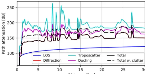
An important property of the total propagation loss (L_band L) is that it is not simply the product (or sum, if logarith-mic representation is used) of the components. Again, we refer to P.452 (ITU-R, 2015) for more details. To give the reader an impression on how the various quantities behave as a function of distance from the transmitter, we have calcu-lated the components for each point in the terrain height pro-file (Fig. 1) and display them in Fig. 2. In contrast to the two-point calculation above, the antenna gains were neglected, as the effective gain towards each point along the path differs somewhat due to the different elevation angles of the path at the two stations. That however requires accounting for the respective antenna patterns, which is supported bypycraf, but beyond the scope of this simple example.

A fast map-making algorithm

With the above approach it is straightforward to produce a path loss map, e.g., around a given transmitter, by sim-ply calculating the propagation loss between each pixel in the map and the Tx location. As the P.452 algorithm is relatively complex, this would however require a substan-tial amount of computing time. In addition, the construc-tion of the geodesics (the shortest paths between two points on the Earth ellipsoid) and SRTM height profile extrac-tion/interpolation are also computationally demanding. Thus, two additional techniques were introduced to provide a sig-nificant speed-up. First, the map computation was moved

(6)

6.2 6.4 6.6 Longitude [deg]6.8 7.0 7.2 7.4 7.6

50.2 50.4 50.6 50.8 51.0 Latitude [deg] 100-m RT Cologne Bonn

100 dB 120 dB 140 dBPath propagation loss160 dB 180 dB 200 dB

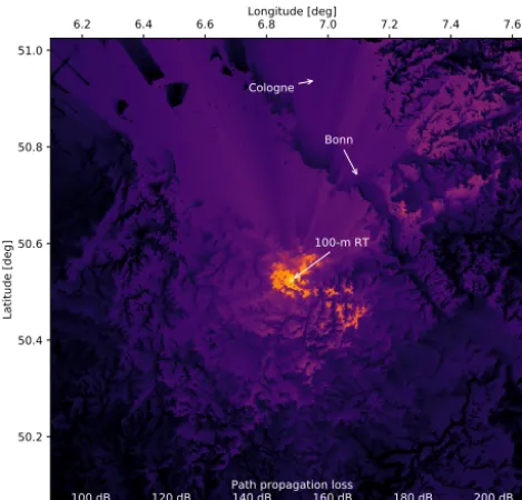
Figure 3. Example map of path propagation losses around the Effelsberg observatory. Based on NASA SRTM data (Farr et al., 2007).

into the Cython part of the code (avoiding the use of slower Python for-loops), where it is furthermore possible to make use of OpenMP9 _{for automatic parallelisation of the code} to improve execution times on machines with many CPU cores. The second improvement is algorithmic in nature and aims to speed-up the geometric part of the computation: the geodesics calculation and height profile generation, which is preparatory work before the actual P.452-algorithm is em-ployed. A path from the map centre to a pixel on the edge of the map crosses many other pixels in-between. We calculate all geodesics between map edge pixels and the centre and use a caching technique to identify the edge-geodesic which comes closest to the pixel centre for each interior pixel. This essentially transforms the problem fromO(n2)toO(n). Un-fortunately, the P.452 algorithm itself can not be treated with a similar technique, because the path elevation angles (and thus also if a path is line-of-sight or trans-horizon) are unique for each pixel as they depend on the terrain height profile be-tween the pixel and the map centre.

Using the attenuation map-making functionality is again a two-step process. First, a helper object is created that caches the terrain and path parameters, which is then fed into the P.452 algorithm, see Listing 3.

Again, we omit the lengthy plot code, but the result of this is visualized in Fig. 3. The hprof_cacheobject is a Python dict-like object containing the cached param-eters and could also be edited by the user before call-ingatten_map_fast. A typical example of such editing

9_{https://www.openmp.org/, last access: 5 June 2018}

the map crosses many other pixels in-between. We calculate all geodesics between map edge pixels and the centre and use a caching technique to identify the edge-geodesic which comes closest to the pixel centre for each interior pixel. This essentially transforms the problem fromO(n2)toO(n). Un-5

fortunately, the P.452 algorithm itself can not be treated with a similar technique, because the path elevation angles (and thus also if a path is line-of-sight or trans-horizon) are unique for each pixel as they depend on the terrain height profile be-tween the pixel and the map centre.

10

Using the attenuation map-making functionality is again a two-step process. First, a helper object is created that caches the terrain and path parameters, which is then fed into the P.452 algorithm:

Listing 1.Fast path propagation loss map-making. 1 import astropy.units as u

15

2 import pycraf.conversions as cnv 3 import pycraf.pathprof as pp 4

5 pp.SrtmConf.set(download=’missing’)

6 20

7 # Effelsberg radio telescope site

8 _{lon_rt = 6.88361 * u.deg}

9 lat_rt = 50.52483 * u.deg

10

11 # Map parameters

25

12 msize_lon, msize_lat = (1, 1) * u.deg

13 _{map_resolution = 3 * u.arcsec}

16 30

17 # P.452 parameters

35

22 _{h_rt, h_tx = (50, 20) * u.m}

23 24

25 hprof_cache = pp.height_map_data(

26 lon_rt, lat_rt,

40

27 msize_lon, msize_lat,

28 map_resolution=map_resolution,

29 zone_t=zone_t, zone_r=zone_r,

30 )

31 45

32 results = pp.atten_map_fast(

33 frequency,

34 temperature,

35 pressure,

36 h_rt, h_tx,

50

37 time_percent,

38 hprof_cache,

39 )

40

41 total_atten = results[’L_b’]

55

Again, we omit the lengthy plot code, but the result of this is visualized in Fig. 3. Thehprof_cache object is a Python dict-like object containing the cached param-eters and could also be edited by the user before call-ingatten_map_fast. A typical example of such editing 60 would be the assignment of a different clutter zone to each of the pixels – given that the user has access to a suitable database containing the true clutter types.

Thepathprofsub-package also provides a large amount of other utility functions, e.g., to plot terrain maps or export 65 maps to a Geographic Information System (GIS) file format such as the Keyhole Markup Language (KML); see online documentation for further information.

3.3 Protection thresholds

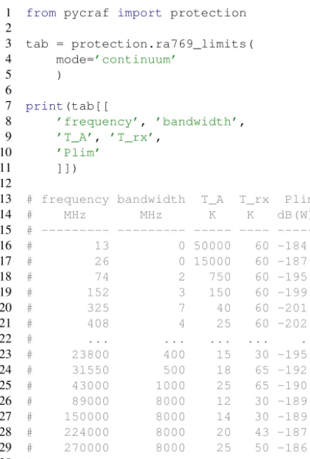
Sincepycrafwas developed for compatibility studies in- 70 volving radio astronomy, the current protection sub-package only offers thresholds relevant in that context. Most importantly, this covers the tables with protection thresholds given in ITU-R Rec. RA.769: Values from this table can

Listing 4.ITU-R Rec. RA.769 thresholds.

6.2 6.4 6.6 Longitude [deg]6.8 7.0 7.2 7.4 7.6

100 dB 120 dB Path propagation loss140 dB 160 dB 180 dB 200 dB

10

11 # Map parameters

12 msize_lon, msize_lat = (1, 1) * u.deg 13 map_resolution = 3 * u.arcsec

14 zone_t = pp.CLUTTER.URBAN 5

15 zone_r = pp.CLUTTER.SUBURBAN 16

18 frequency = 10 * u.GHz 19 temperature = 290 * u.K 10

20 pressure = 1013 * u.hPa 21 time_percent = 2 * u.percent 22 h_rt, h_tx = (50, 20) * u.m 23

24 15

25 hprof_cache = pp.height_map_data( 26 lon_rt, lat_rt,

28 map_resolution=map_resolution, 29 zone_t=zone_t, zone_r=zone_r, 20

30 )

31

33 frequency,

34 temperature,

25

35 pressure,

36 h_rt, h_tx,

37 time_percent,

38 hprof_cache,

39 )

30 40

Again, we omit the lengthy plot code, but the result of this is visualized in Fig. 3. The hprof_cacheobject is a Python dict-like object containing the cached param- 35 eters and could also be edited by the user before call-ingatten_map_fast. A typical example of such editing would be the assignment of a different clutter zone to each of the pixels – given that the user has access to a suitable database containing the true clutter types. 40

Thepathprofsub-package also provides a large amount of other utility functions, e.g., to plot terrain maps or export maps to a Geographic Information System (GIS) file format such as the Keyhole Markup Language (KML); see online documentation for further information. 45

Sincepycraf was developed for compatibility studies in-volving radio astronomy, the current protection sub-package only offers thresholds relevant in that context. Most importantly, this covers the tables with protection thresholds 50 given in ITU-R Rec. RA.769:

Listing 4.ITU-R Rec. RA.769 thresholds. 1 from pycraf import protection 2

3 tab = protection.ra769_limits(

4 mode=’continuum’ 55

5 )

6

7 print(tab[[

8 ’frequency’, ’bandwidth’,

9 ’T_A’, ’T_rx’, 60

10 ’Plim’

11 ]])

12

13 # frequency bandwidth T_A T_rx Plim

14 # MHz MHz K K dB(W) 65

15 # --- --- --- ----

---16 # 13 0 50000 60 -184.6

17 # 26 0 15000 60 -187.9

18 # 74 2 750 60 -195.0

19 # 152 3 150 60 -199.5 70

20 # 325 7 40 60 -201.0

21 # 408 4 25 60 -202.9

22 # ... ... ... ... ...

23 # 23800 400 15 30 -195.6

24 # 31550 500 18 65 -192.4 75

25 # 43000 1000 25 65 -190.6

26 # 89000 8000 12 30 -189.4

27 # 150000 8000 14 30 -189.2

28 # 224000 8000 20 43 -187.6

29 # 270000 8000 25 50 -186.8 80

30 # Length = 21 rows

Values from this table can then subsequently be used to com-pare received power levels of a potential interferer with the permitted power levels. Almost all compatibility studies that involve RAS refer to the RA.769 methodology or thresholds 85 in one form or another.

Adv. Radio Sci., 16, 1–17, 2018 www.adv-radio-sci.net/16/1/2018/ then subsequently be used to compare received power levels 75 of a potential interferer with the permitted power levels.

Al-Adv. Radio Sci., 16, 1–18, 2018 www.adv-radio-sci.net/16/1/2018/ Listing 3.Fast path propagation loss map-making.

would be the assignment of a different clutter zone to each of the pixels – given that the user has access to a suitable database containing the true clutter types.

Thepathprofsub-package also provides a large amount of other utility functions, e.g., to plot terrain maps or export maps to a Geographic Information System (GIS) file format such as the Keyhole Markup Language (KML); see online documentation for further information.

Sincepycrafwas developed for compatibility studies in-volving radio astronomy, the current protection

(7)

package only offers thresholds relevant in that context. Most importantly, this covers the tables with protection thresholds given in ITU-R Rec. RA.769 (ITU-R, 2003), see Listing 4.

6.2 6.4 6.6 Longitude [deg]6.8 7.0 7.2 7.4 7.6

50.2 50.4 50.6 50.8 51.0

Latitude [deg]

100-m RT Cologne

Bonn

100 dB 120 dB 140 dBPath propagation loss160 dB 180 dB 200 dB

10

11 # Map parameters

12 _{msize_lon, msize_lat = (1, 1) * u.deg}

13 map_resolution = 3 * u.arcsec

5

16

10

22 h_rt, h_tx = (50, 20) * u.m

23 24 15

25 hprof_cache = pp.height_map_data(

26 lon_rt, lat_rt,

28 map_resolution=map_resolution,

29 zone_t=zone_t, zone_r=zone_r,

20

30 )

31

33 frequency,

34 temperature,

25

35 pressure,

36 h_rt, h_tx,

37 time_percent,

38 hprof_cache,

39 )

30 40

Again, we omit the lengthy plot code, but the result of this is visualized in Fig. 3. The hprof_cache object is a Python dict-like object containing the cached param- 35 eters and could also be edited by the user before call-ingatten_map_fast. A typical example of such editing would be the assignment of a different clutter zone to each of the pixels – given that the user has access to a suitable database containing the true clutter types. 40

Since pycrafwas developed for compatibility studies in-volving radio astronomy, the current protection sub-package only offers thresholds relevant in that context. Most importantly, this covers the tables with protection thresholds 50 given in ITU-R Rec. RA.769:

Listing 4.ITU-R Rec. RA.769 thresholds.

1 from pycraf import protection

2

5 )

6

7 print(tab[[

9 ’T_A’, ’T_rx’, 60

10 ’Plim’

11 ]])

12

15 # --- --- --- ----

---16 # 13 0 50000 60 -184.6

17 # 26 0 15000 60 -187.9

18 # 74 2 750 60 -195.0

19 # 152 3 150 60 -199.5 70

20 # 325 7 40 60 -201.0

21 # 408 4 25 60 -202.9

22 # ... ... ... ... ...

23 # 23800 400 15 30 -195.6

24 # 31550 500 18 65 -192.4 75

25 # 43000 1000 25 65 -190.6

26 # 89000 8000 12 30 -189.4

27 # 150000 8000 14 30 -189.2

28 # 224000 8000 20 43 -187.6

29 # 270000 8000 25 50 -186.8 80 30 # Length = 21 rows

Adv. Radio Sci., 16, 1–17, 2018 www.adv-radio-sci.net/16/1/2018/ Listing 4.ITU-R Rec. RA.769 (ITU-R, 2003) thresholds.

Values from this table can then subsequently be used to com-pare received power levels of a potential interferer with the permitted power levels. Almost all compatibility studies that involve RAS refer to the RA.769 methodology or thresholds in one form or another.

3.4 Antenna patterns

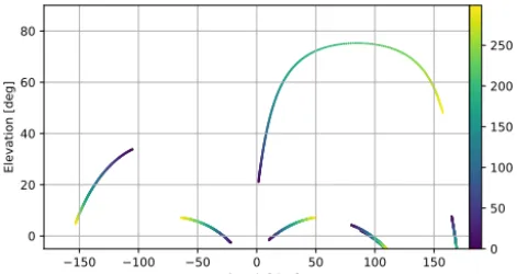
In many realistic compatibility studies, the antenna patterns of transmitter and receiver have to be accounted for. This can be more complex than what might be naively assumed. For example, the base stations and partly also the user equipment of the next-generation mobile communications standard 5G will utilize phased array antennas. To calculate the effective gain for the propagation path, one must account for the di-rection of the formed beam, the orientation (and rotation) of the antenna frame normal vector, and the relative position of the propagation path with respect to the antenna frame. We will return to this in Sect. 4.

75 50 25 0 25 50 75 Azimuth [deg] 80

60 40 20 0 20 40 60 80

Elevation [deg]

Escan: 0.0d, Tilt: 0.0d

75 50 25 0 25 50 75 Azimuth [deg] 80

60 40 20 0 20 40 60 80

Elevation [deg]

75 50 25 0 25 50 75 Azimuth [deg] 80

60 40 20 0 20 40 60 80

Elevation [deg]

75 50 25 0 25 50 75 Azimuth [deg] 80

60 40 20 0 20 40 60 80

Elevation [deg]

20 10 0 10 20

Gain [dB]

Figure 4. Composite phased-array antenna patterns of the next mobile-communications standard 5G as defined in ITU-R ITU-Rec. M.2101 (ITU-ITU-R, 2017a).

Inpycrafseveral (simplified) antenna models are pro-vided that implement various ITU-R recommendations, which shall be used for spectrum management studies. As an example, the fairly complex 5G composite antenna pat-terns can be obtained as demonstrated in Listing 5, where theazim_iandelev_jangles define the pointing of the formed beam in the antenna frame coordinates (azimuth and elevation). In Fig. 4 examples are shown for four different beam directions:(0,0◦),(30,0◦),(0,15◦), and(30,15◦).

3.5 Atmospheric attenuation

Once the propagation path exceeds a certain length, e.g., for communication links to satellites or for radio-astronomical observation of extra-terrestrial sources, the attenuation by the gases in the atmosphere of the Earth becomes impor-tant, especially at higher frequencies. Again, there exists a ITU-R recommendation, P.676, which was implemented in theatm sub-package. It can be used to predict the attenu-ation as a function of frequency, path geometry, and atmo-spheric parameters. The two molecules that play a major role are oxygen (so-called dry component) and water (wet component), both introducing spectral-line emission and ab-sorption. Furthermore, oxygen also produces the continuous non-resonant Debye-spectrum (below 10 GHz). At frequen-cies above 100 GHz continuous attenuation by nitrogen starts to play a role as well.

The calculation of atmospheric attenuation is performed via a ray-tracing approach. Let us assume a radio signal enters Earth’s atmosphere and travels to a receiving station close to the ground. First, the atmosphere is divided into

(8)

184 B. Winkel and A. Jessner: Spectrum management and compatibility studies with Python B. Winkel and A. Jessner: Spectrum management and compatibility studies with Python 7

Listing 4.ITU-R Rec. RA.769 thresholds. 6.2 6.4 6.6 Longitude [deg]6.8 7.0 7.2 7.4 7.6

100 dB 120 dB 140 dB 160 dB 180 dB 200 dB Path propagation loss

10

11 # Map parameters

12 msize_lon, msize_lat = (1, 1) * u.deg 13 map_resolution = 3 * u.arcsec

14 zone_t = pp.CLUTTER.URBAN 5

15 zone_r = pp.CLUTTER.SUBURBAN 16

17 # P.452 parameters 18 frequency = 10 * u.GHz 19 temperature = 290 * u.K 10

20 pressure = 1013 * u.hPa 21 time_percent = 2 * u.percent 22 h_rt, h_tx = (50, 20) * u.m 23

24 15

25 hprof_cache = pp.height_map_data( 26 lon_rt, lat_rt,

28 map_resolution=map_resolution, 29 zone_t=zone_t, zone_r=zone_r, 20

30 )

31

32 results = pp.atten_map_fast( 33 frequency,

34 temperature, 25

35 pressure, 36 h_rt, h_tx, 37 time_percent, 38 hprof_cache,

39 )

30 40

Again, we omit the lengthy plot code, but the result of this is visualized in Fig. 3. Thehprof_cacheobject is a Python dict-like object containing the cached param- 35 eters and could also be edited by the user before call-ingatten_map_fast. A typical example of such editing would be the assignment of a different clutter zone to each of the pixels – given that the user has access to a suitable database containing the true clutter types. 40

Sincepycrafwas developed for compatibility studies in-volving radio astronomy, the current protection sub-package only offers thresholds relevant in that context. Most importantly, this covers the tables with protection thresholds 50 given in ITU-R Rec. RA.769:

Listing 4.ITU-R Rec. RA.769 thresholds. 1 from pycraf import protection 2

5 )

6

7 print(tab[[

9 ’T_A’, ’T_rx’, 60

10 ’Plim’

11 ]])

12

15 # --- --- --- ----

---16 # 13 0 50000 60 -184.6

17 # 26 0 15000 60 -187.9

18 # 74 2 750 60 -195.0

19 # 152 3 150 60 -199.5 70

20 # 325 7 40 60 -201.0

21 # 408 4 25 60 -202.9

22 # ... ... ... ... ...

23 # 23800 400 15 30 -195.6

24 # 31550 500 18 65 -192.4 75

25 # 43000 1000 25 65 -190.6

26 # 89000 8000 12 30 -189.4

27 # 150000 8000 14 30 -189.2

28 # 224000 8000 20 43 -187.6

29 # 270000 8000 25 50 -186.8 80

30 # Length = 21 rows

Adv. Radio Sci., 16, 1–17, 2018 www.adv-radio-sci.net/16/1/2018/

75 50 25 0 25 50 75 Azimuth [deg] 80 60 40 20 0 20 40 60 80 Elevation [deg]

20 10 0 10 20 Gain [dB]

Figure 4. Composite phased-array antenna patterns of the next mobile-communications standard 5G as defined in ITU-R ITU-Rec. M.2101.

Listing 1.5G composite antenna patterns.

1 import numpy as np

3 import pycraf.conversions as cnv 4 import pycraf.antenna as ant

5 5

6 azims = np.arange(-180, 180) * u.deg

7 elevs = np.arange(-90, 90) * u.deg

8

9 # antenna parameters according to

10 # ITU-R Rec. M.2101 10

11 G_Emax = 5 * cnv.dB

12 A_m, SLA_nu = (30, 30) * cnv.dimless

13 azim_3db, elev_3db = (65, 65) * u.deg

14 d_H, d_V = (0.5, 0.5) * cnv.dimless

15 N_H, N_V = 8, 8 15

16

17 azim_i, elev_j = (0, 0) * u.deg

18

19 gains = ant.imt2020_composite_pattern(

20 azims[np.newaxis], 20

21 elevs[:, np.newaxis],

22 azim_i, elev_j,

23 G_Emax,

24 A_m, SLA_nu,

25 azim_3db, elev_3db, 25

26 d_H, d_V,

27 N_H, N_V,

28 )

where the azim_i and elev_jangles define the point-ing of the formed beam in the antenna frame coordinates 30 (azimuth and elevation). In Fig. 4 examples are shown for four different beam directions:(0,0◦_),_(30,0◦_),_(0,15◦_{), and} (30,15◦).

3.5 Atmospheric attenuation

Once the propagation path exceeds a certain length, e.g., for 35 communication links to satellites or for radio-astronomical observation of extra-terrestrial sources, the attenuation by the gases in the atmosphere of the Earth becomes impor-tant, especially at higher frequencies. Again, there exists a ITU-R recommendation, P.676, which was implemented in 40 the atmsub-package. It can be used to predict the attenu-ation as a function of frequency, path geometry, and atmo-spheric parameters. The two molecules that play a major role are oxygen (so-called dry component) and water (wet component), both introducing spectral-line emission and ab- 45 sorption. Furthermore, oxygen also produces the continuous non-resonant Debye-spectrum (below 10 GHz). At frequen-cies above 100 GHz continuous attenuation by nitrogen starts to play a role as well.

The calculation of atmospheric attenuation is performed 50 via a ray-tracing approach. Let us assume a radio signal enters Earth’s atmosphere and travels to a receiving station close to the ground. First, the atmosphere is divided into lay-ers (several hundreds or more) and for each of these the atten-uation of the incident signal is calculated, such that the sig- 55

Listing 5.5G composite antenna patterns.

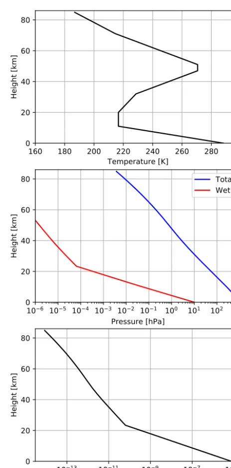
ers (several hundreds or more) and for each of these the atten-uation of the incident signal is calculated, such that the sig-nal, which leaves a layer is somewhat weaker than the signal that entered a layer. At the same time, the layer itself emits radio waves having the aforementioned spectral properties. Each layer has different physical properties, such as temper-ature, pressure, water content, and refractivity. These “height profiles” have to be known to calculate the specific attenua-tion per layer. For ITU-R related studies, it is widely accepted to work with mean profiles, which were averaged over a year. The “standard profile” is provided in ITU-R Rec. P.835 (ITU-R, 2012) along with five more specialised profiles, associated with the geographic latitude and season (“high-latitude sum-mer/winter”, “mid-latitude sumsum-mer/winter”, and “low lati-tude”). For example:

160 180 200 220 240 260 280 300 Temperature [K] 0 20 40 60 80 Height [km]

10 6 ₁₀ 5 ₁₀ 4 ₁₀ 3 ₁₀ 2 ₁₀ 1 ₁₀0 ₁₀1 ₁₀2 ₁₀3

Pressure [hPa] 0 20 40 60 80 Height [km] Total Wet

10 13 ₁₀ 11 ₁₀ 9 ₁₀ 7 ₁₀ 5

Water density [g cm ] 0 20 40 60 80 Height [km] 3

Figure 5.Standard atmospheric height profiles (temperature, pres-sure, and water density) according to ITU-R Rec. P.835 (ITU-R, 2012).

(9)

B. Winkel and A. Jessner: Spectrum management and compatibility studies with Python 185 “mid-latitude summer/winter”, and “low latitude”). For

ex-ample:

Listing 6.Atmospheric attenuation. 1 import numpy as np

3 import pycraf.conversions as cnv

5

4 from pycraf import atm

5

6 # define height grid

7 height_grid = np.arange(0, 85, 0.1) * u.km

8 10

9 # query profile_standard function

10 (

11 temperatures,

12 pressures,

13 rho_water,

15

14 pressures_water,

15 ref_indices,

16 humidities_water,

17 humidities_ice

18 ) = atm.profile_standard(height_grid)

20

The resulting profiles are displayed in Fig. 5. ITU-R ITU-Rec. P.676 contains tables with the resonance lines of oxygen and water, necessary to calculate the specific at-tenuation for one layer (or propagation paths close to the ground, which stay in a single layer). The function

25

atten_specific_annex1can be used for that:

18 freqs = np.arange(1, 1000) * u.GHz

19 p_total = 1013 * u.hPa

20 temperature = 290 * u.K

21 rho_water = 7.5 * u.g / u.m ** 3

30 22

23 # need dry and wet pressure separately:

24 p_wet = atm.pressure_water_from_rho_water(

25 temperature, rho_water

26 )

35

27 p_dry = p_total - p_wet

28

29 print(’O2 pressure: {:.2f}’.format(p_dry)) 30 print(’H2O vapor partial pressure: ’

31 ’{:.2f}’.format(p_wet))

40

32 # Oxygen pressure: 1002.96 hPa

33 # Water vapor partial pressure: 10.04 hPa

34

35 a_dry, a_wet = atm.atten_specific_annex1(

36 freqs, p_dry, p_wet, temperature

45

37 )

The resulting spectrum is shown in Fig. 6. Calculating such spectra for each layer allows us to perform the ray-tracing for a slant path through the full atmosphere (with the functionatten_slant_annex1):

50

37 elevation = 15 * u.deg

38 station_altitude = 300 * u.m

39 freqs = np.arange(1, 100, 0.1) * u.GHz

40

41 (

55

160 180 200 220 240 260 280 300 Temperature [K]

0 20 40 60 80

Height [km]

10 6 ₁₀ 5 ₁₀ 4 ₁₀ 3 ₁₀ 2 ₁₀ 1 ₁₀0 ₁₀1 ₁₀2 ₁₀3

Pressure [hPa] 0

20 40 60 80

Height [km]

Total Wet

10 13 ₁₀ 11 ₁₀ 9 ₁₀ 7 ₁₀ 5

Water density [g cm ] 0

20 40 60 80

Height [km]

3

Figure 5.Standard atmospheric height profiles (temperature, pres-sure, and water density) according to ITU-R Rec. P.835.

42 total_atten, refraction, tebb

43 ) = atm.atten_slant_annex1(

44 freqs, elevation,

45 station_altitude,

46 atm.profile_highlat_winter 60

47 )

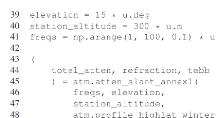
In Fig. 7 the total atmospheric attenuation of a slant path for Summer/Winter high-latitude standard profiles is pre-sented, along the so-called equivalent-black-body tempera-ture,T_ebb, of the full atmosphere with major contributions by 65

the atmospheric emission itself.

Adv. Radio Sci., 16, 1–17, 2018 www.adv-radio-sci.net/16/1/2018/

Listing 6.Atmospheric attenuation.

The resulting profiles are displayed in Fig. 5. ITU-R ITU-Rec. P.676 (ITU-ITU-R, 2013) contains tables with the resonance lines of oxygen and water, necessary to calculate the specific attenuation for one layer (or propagation paths close to the ground, which stay in a single layer). The func-tion atten_specific_annex1 can be used for that: 19 _{freqs = np.arange(1, 1000) * u.GHz}

20 _{p_total = 1013 * u.hPa} 21 _{temperature = 290 * u.K}

22 _{rho_water = 7.5 * u.g / u.m ** 3} 23

24 # need dry and wet pressure separately: 25 p_wet = atm.pressure_water_from_rho_water( 26 temperature, rho_water

27 )

28 p_dry = p_total - p_wet 29

30 print(’O2 pressure: {:.2f}’.format(p_dry)) 31 print(’H2O vapor partial pressure: ’

32 ’{:.2f}’.format(p_wet))

33 # Oxygen pressure: 1002.96 hPa

34 # Water vapor partial pressure: 10.04 hPa 35

36 a_dry, a_wet = atm.atten_specific_annex1( 37 freqs, p_dry, p_wet, temperature

38 )

The resulting spectrum is shown in Fig. 6. Calculating such spectra for each layer allows us to perform the ray-tracing for a slant path through the full atmosphere (with the functionatten_slant_annex1):

0 200 400 600 800

Frequency [GHz] 102

101 100 101 102 103 104

Specific attenuation [dB / km]

Dry air Wet air Total

Figure 6.Specific attenuation for a layer with a total pressure of 1013 hPa, a temperature of 290 K, and a specific water density of 7.5 g cm−3according to ITU-R Rec. P.676 (ITU-R, 2013).

39 _{elevation = 15 * u.deg} 40 _{station_altitude = 300 * u.m}

41 _{freqs = np.arange(1, 100, 0.1) * u.GHz} 42

43 (

44 total_atten, refraction, tebb 45 ) = atm.atten_slant_annex1( 46 freqs, elevation, 47 station_altitude,

48 atm.profile_highlat_winter

49 )

In Fig. 7 the total atmospheric attenuation of a slant path for Summer/Winter high-latitude standard profiles is pre-sented, along the so-called equivalent-black-body tempera-ture,Tebb, of the full atmosphere with major contributions by the atmospheric emission itself.

3.6 Satellite two-line elements

For studies involving a satellite or a satellite network it is often necessary to determine their position relative to an Earth station. Satellite orbits vary slowly in time as a consequence of the gravitational influence of planetary system bodies, most importantly the Moon, the Sun, and Jupiter. Furthermore, the orbits are subject to drag forces induced by the outer layers of the atmosphere, especially, in the case of low-earth orbit (LEO) satellites. Satellites are therefore constantly monitored by stations on Earth to update their orbital parameters. These are provided in a standardized format, the so-called two-line element (TLE) sets, which are usually updated once per day and can be retrieved from the Space Track10 _{or CelesTrak}11 websites. As an example, the TLE of the International Space Station (ISS) for 20 September 2008 looks like this:

10_{https://www.space-track.org, last access: 5 June 2018} 11_{http://celestrak.com/, last access: 5 June 2018}