A comparative study on the convergence rate of some iteration methods involving contractive mappings

(1)

R E S E A R C H

Open Access

A comparative study on the convergence

rate of some iteration methods involving

contractive mappings

Shahin Fathollahi

1

_{, Adrian Ghiura}

2

_{, Mihai Postolache}

2*

_{and Shahram Rezapour}

1

*_{Correspondence:}

[email protected]

2_{Department of Mathematics and}

Informatics, University Politehnica of Bucharest, Bucharest, 060042, Romania

Full list of author information is available at the end of the article

Abstract

We compare the rate of convergence for some iteration methods for contractions. We conclude that the coeﬃcients involved in these methods have an important role to play in determining the speed of the convergence. By using Matlab software, we provide numerical examples to illustrate the results. Also, we compare mathematical and computer-calculating insights in the examples to explain the reason of the existence of the old diﬀerence between the points of view.

MSC: 47H09; 47H10

Keywords: contractive map; ﬁxed point; iteration method; rate of convergence

1 Introduction

Iteration schemes for numerical reckoning ﬁxed points of various classes of nonlinear op-erators are available in the literature. The class of contractive mappings via iteration meth-ods is extensively studied in this regard. In , Plunkett published a paper on the rate of convergence for relaxation methods []. In , Bowden presented a talk in a symposium on digital computing machines entitled ‘Faster than thought’ []. Later, this basic idea has been used in engineering, statistics, numerical analysis, approximation theory, and physics for many years (see, for example, [–] and []). In , Argyros published a paper about iterations converging faster than Newton’s method to the solutions of nonlinear equations in Banach spaces [, ]. In , Lucet presented a method faster than the fast Legen-dre transform []. In , Berinde used the notion of rate of convergence for iterations method and showed that the Picard iteration converges faster than the Mann iteration for a class of quasi-contractive operators []. Later, he provided some results in this area [, ]. In , Babu and Vara Prasad showed that the Mann iteration converges faster than the Ishikawa iteration for the class of Zamﬁrescu operators []. In , Popescu showed that the Picard iteration converges faster than the Mann iteration for the class of quasi-contractive operators []. Recently, there have been published some papers about introducing some new iterations and comparing of the rates of convergence for some it-eration methods (see, for example, [–] and []).

In this paper, we compare the rates of convergence of some iteration methods for con-tractions and show that the involved coeﬃcients in such methods have an important role

(2)

to play in determining the rate of convergence. During the preparation of this work, we found that the eﬃciency of coeﬃcients had been considered in [] and []. But we ob-tained our results independently, before reading these works, and one can see it by com-paring our results and those ones.

2 Preliminaries

As we know, the Picard iteration has been extensively used in many works from diﬀerent points of view. Let (X,d) be a metric space,x∈X, andT: X→Xa selfmap. The Picard iteration is deﬁned by

xn+=Txn

for alln≥. Let{αn}n≥,{βn}n≥, and{γn}n≥be sequences in [, ]. Then the Mann iter-ation method is deﬁned by

xn+=αnxn+ ( –αn)Txn (.)

for alln≥ (for more information, see []). Also, the Ishikawa iteration method is de-ﬁned by

xn+= ( –αn)xn+αnTyn,

yn= ( –βn)xn+βnTxn

(.)

for all n≥ (for more information, see []). The Noor iteration method is deﬁned by

yn= ( –βn)xn+βnTzn, (.)

zn= ( –γn)xn+γnTxn

for alln≥ (for more information, see []). In , Agarwalet al.deﬁned their new iteration methods by

xn+= ( –αn)Txn+αnTyn,

yn= ( –βn)xn+βnTxn

(.)

for all n≥ (for more information, see []). In , Abbaset al.deﬁned their new iteration methods by

xn+= ( –αn)Tyn+αnTzn,

yn= ( –βn)Txn+βnTzn, (.)

(3)

for alln≥ (for more information, see []). In , Thakuret al.deﬁned their new iteration methods by

yn= ( –βn)zn+βnTzn, (.)

for alln≥ (for more information, see []). Also, the Picard S-iteration was deﬁned by

xn+=Tyn,

yn= ( –βn)Txn+βnTzn, (.)

for alln≥ (for more information, see [] and []).

3 Self-comparing of iteration methods

Now, we are ready to provide our main results for contractive maps. In this respect, we assume that (X,·) is a normed space,x∈X,T:X→Xis a selfmap and{αn}n≥,{βn}n≥ and{γn}n≥are sequences in (, ).

The Mann iteration is given byxn+= ( –αn)xn+αnTxnfor alln≥.

Note that we can rewrite it asxn+=αnxn+ ( –αn)Txnfor alln≥.

We call these cases the ﬁrst and second forms of the Mann iteration method.

In the next result we show that choosing a type of sequence{αn}n≥in the Mann iteration has a notable role to play in the rate of convergence of the sequence{xn}n≥.

Let{un}n≥ and{vn}n≥ be two ﬁxed point iteration procedures that converge to the same ﬁxed pointpandun–p ≤anandvn–p ≤bnfor alln≥. If the sequences

{an}n≥and{bn}n≥converge toaandb, respectively, andlimn→∞abn–n–ab= , then we say that{un}n≥converges faster than{vn}n≥top(see [] and []).

Proposition . Let C be a nonempty,closed,and convex subset of a Banach space X, x∈C,T:C→C a contraction with constant k∈(, )and p a fixed point of T.Consider the first case for Mann iteration.If the coefficients of Txnare greater than the coefficients

of xn,that is,  –αn<αnfor all n≥or equivalently{αn}n≥is a sequence in(_, ),then the Mann iteration converges faster than the Mann iteration which the coeﬃcients of xnare

greater than the coeﬃcients of Txn.

Proof Let{xn}be the sequence in the Mann iteration which the coeﬃcients ofTxnare

greater than the coeﬃcients ofxn, that is,

xn+= ( –αn)xn+αnTxn (.)

for alln. In this case, we have

xn+–p=( –αn)xn+αnTxn–p≤( –αn)xn–p+αnTxn–p

≤ –αn( –k)

(4)

for alln. Sinceαn∈(_, ),  –αn( –k) <  –_( –k). Putan= ( –_( –k))nx–pfor

alln. Now, let{xn}be the sequence in the Mann iteration of which the coeﬃcients ofxn

are greater than the coeﬃcients ofTxn. In this case, we have

xn+–p=αnxn+ ( –αn)Txn–p≤αnxn–p+ ( –αn)Txn–p

≤ – ( –αn)( –k)

xn–p

for alln. Since  –αn<αnfor alln≥, we get  – ( –αn)( –k) <  for alln≥. Putbn=

x–pfor alln. Note thatliman

bn =lim

(–(–k))nx–p

x–p = . This completes the proof.

Note that we can use  –αn<αn, fornlarge enough, instead of the condition  –αn<αn,

for alln≥. One can use similar conditions instead of the conditions which we will use in our results.

As we know, we can consider four cases for writing the Ishikawa iteration method. In the next result, we indicate each case by different enumeration. Similar to the last result, we want to compare the Ishikawa iteration method with itself in the four possible cases. Again, we show that the coefficient sequences{αn}n≥and{βn}n≥have effective roles to play in the rate of convergence of the sequence{xn}n≥in the Ishikawa iteration method.

Proposition . Let C be a nonempty, closed, and convex subset of a Banach space X, x∈C,T: C→C a contraction with constant k∈(, ),and p a ﬁxed point of T.Consider the following cases of the Ishikawa iteration method:

yn= ( –βn)xn+βnTxn,

(.)

xn+=αnxn+ ( –αn)Tyn,

yn=βnxn+ ( –βn)Txn,

(.)

xn+=αnxn+ ( –αn)Tyn,

(.)

and

yn=βnxn+ ( –βn)Txn

(.)

for all n≥.If –αn<αnand –βn<βnfor all n≥,then the case(.)converges faster

than the others.In fact,the Ishikawa iteration method is faster whenever the coeﬃcients of Tynand Txnsimultaneously are greater than the related coeﬃcients of xnfor all n≥.

Proof Let{xn}n≥be the sequence in the case (.). Then we have

yn–p=( –βn)xn+βnTxn–p

≤( –βn)xn–p+βnTxn–p

≤( –βn) +βnk

(5)

and

xn+–p=( –αn)xn+αnTyn–p

≤( –αn)xn–p+αnTyn–p

≤( –αn)xn–p+kαnyn–p

≤ –αn+kαn

( –βn) +βnk

xn–p

≤ –αn+αnk–αnβnk+αnβnk

xn–p

≤ –αn( –k) –αnβnk( –k)

xn–p

for alln≥. Sinceαn,βn∈(_, ),  –αn( –k) –αnβnk( –k) <  –_( –k) –_k( –k) for

alln≥. Putan= ( –_( –k) –_k( –k))nx–pfor alln≥. If{xn}n≥is the sequence in the case (.), then we get

yn–p=βnxn+ ( –βn)Txn–p

≤βnxn–p+ ( –βn)Txn–p

≤ – ( –βn)( –k)

xn–p

and

xn+–p=αnxn+ ( –αn)Tyn–p

≤αnxn–p+ ( –αn)Tyn–p

≤αnxn–p+k( –αn)yn–p

≤αn+k( –αn)

 – ( –βn)( –k)

xn–p

=αn+ ( –αn)k–k( –αn)( –βn)( –k)

xn–p

= – ( –αn)( –k) – ( –αn)( –βn)k( –k)

xn–p

for alln≥. Sinceαn,βn∈(_, ),  – ( –αn)( –k) – ( –αn)( –βn)( –k) <  for alln≥.

Putbn=x–pfor alln≥. Since

 –

( –k) – 

k(k– ) <  + 

k( –k),

we get liman

bn =lim

(–(–k)–k(–k))nx–p

x–p =  and so the iteration (.) converges faster

than the case (.). Now, let{xn}n≥be the sequence in the case (.). Then

yn–p=βxn+ ( –βn)Txn–p

≤βnxn–p+ ( –βn)Txn–p

≤βn+k( –βn)

xn–p

= – ( –βn)( –k)

(6)

and

≤( –αn)xn–p+αnTyn–p

 – ( –βn)( –k)

xn–p

= –αn+kαn–αn( –βn)k( –k)

xn–p

= –αn( –k) –αn( –βn)k( –k)

xn–p

for alln≥. Sinceαn,βn∈(_, ) for alln≥, –( –k) < –αn( –k) < –_( –k) and–_k( –

k) < –αn( –βn)k( –k) <  for alln. Hence,

 –αn( –k) –αn( –βn)k( –k) <  –

 ( –k)

for alln≥. Putcn= ( –_( –k))nx–pfor alln≥. Thus, we obtain

liman

cn

=lim( –



( –k) – 

k( –k))nx–p ( –_( –k))n_x

–p

= 

and so the iteration (.) converges faster than the case (.). Now, let{xn}n≥be the se-quence in the case (.). Then we have

yn–p=( –β)xn+βnTxn–p

≤( –βn)xn–p+βnTxn–p

≤ –βn( –k)

xn–p

and

xn+–p=αnxn+ ( –αn)Tyn

≤αnxn–p+ ( –αn)Tyn–p

≤αnxn–p+k( –αn)yn–p

≤αn+k( –αn)

 –βn( –k)

xn–p

≤αn+k( –αn) – ( –αn)βnk( –k)

xn–p

≤ – ( –αn) +k( –αn) – ( –αn)βnk( –k)

xn–p

≤ – ( –αn)( –k) – ( –αn)βnk( –k)

xn–p

for alln≥. Sinceαn,βn∈(_, ) for alln, –( –k) < –αn( –k) < –_( –k), and –_k( –

k) < –( –αn)βnk( –k) <  and so

 –αn( –k) – ( –αn)βnk( –k) <  –

(7)

for alln≥. Putdn= ( –_( –k))nx–pfor alln≥. Then we have

liman

dn

=lim( –



( –k) – 

k( –k))

n_x_–_p

( –_( –k))n_x_–_p = 

and so the iteration (.) converges faster than the case (.).

By using a similar condition, one can show that the iteration (.) is faster than the case (.).

Now consider eight cases for writing the Noor iteration method. By using a condition, we show that the coeﬃcient sequences{αn}n≥,{βn}n≥, and{γn}n≥have eﬀective roles to play in the rate of convergence of the sequence{xn}n≥in the Noor iteration method. We enumerate the cases of the Noor iteration method during the proof of our next re-sult.

Theorem . Let C be a nonempty,closed,and convex subset of a Banach space X,x∈C, T:C→C a contraction with constant k∈(, )and p a ﬁxed point of T.Consider the case (.)of the Noor iteration method

⎧ ⎪ ⎨ ⎪ ⎩

yn= ( –βn)xn+βnTzn,

for all n≥.If –αn<αn,  –βn<βn,and –γn<γnfor all n≥,then the iteration(.)

is faster than the other possible cases.

Proof First, we compare the case (.) with the following Noor iteration case: ⎧

⎪ ⎨ ⎪ ⎩

un+= ( –αn)un+αnTvn,

vn= ( –βn)un+βnTwn,

wn=γnun+ ( –γn)Tun

(.)

for alln≥. Note that

zn–p=( –γn)xn+γnTxn–p

≤( –γn)xn–p+kγnxn–p

= – ( –k)γn

xn–p

and

yn–p=( –βn)xn+βnTzn–p

≤( –βn)xn–p+kβnzn–p

≤( –βn) +kβn

 – ( –k)γn

xn–p

≤ –βn( –k) –βnγnk( –k)

(8)

for alln≥. Also, we have

≤( –αn)xn–p+kαnyn–p

≤( –αn)xn–p+kαn

 –βn( –k) –βnγnk( –k)

xn–p

 –βn( –k) –βnγnk( –k)

xn–p

≤ –αn+kαn–k( –k)βnαn–αnβnγnk( –k)

xn–p

≤ – ( –k)αn–k( –k)βnαn–αnβnγnk( –k)

xn–p

for alln≥. Sinceαn,βn,γn∈(, ) for alln, –( –k) < –αn( –k) < –( –k), –k( –k) < –αnβnk( –k) < –_k( –k), and

–k( –k) < –αnβnγnk( –k) < –

 k

_{( –}_k)

for alln. This implies that

 – ( –k)αn–k( –k)βnαn–αnβnγnk( –k) <  –



( –k) – 

k( –k) –  k

_{( –}_k)

for alln. Putan= ( –_( –k) –_k( –k))nx–pfor alln≥. Now for the sequences {un}n≥withu=xand{vn}n≥in (.), we have

wn–p=γnun+ ( –γn)Tun–p

≤γnun–p+k( –γn)un–p

= – ( –γn)( –k)

un–p

and

vn–p=( –βn)un+βnTwn–p

≤( –βn)un–p+kβnwn–p

≤( –βn) +kβn

 – ( –γn)( –k)

un–p

≤ –βn+kβn–βn( –γn)k( –k)

un–p

≤ –βn( –k) –βn( –γn)k( –k)

un–p

for alln≥. Hence,

un+–p=( –αn)un+αnTvn–p

≤( –αn)un–p+kαnvn–p

≤( –αn)un–p+kαn

 –βn( –k) –βn( –γn)k( –k)

un–p

≤( –αn) +kαn–αnβnk( –k) –αβn( –γn)K( –k)

un–p

≤ –αn( –k) –αnβnk( –k) –αβn( –γn)K( –k)

(9)

for alln. Sinceαn,βn,γn∈(_, ) for alln, –k( –k) < –αnβnk( –k) < –_k( –k) and_k( –

k) < –αnβn( –γn)k( –k) <  for alln. Hence,

 –αn( –k) –αnβnk( –k) –αβn( –γn)k( –k) <  –



( –k) –  k( –k)

for alln. Putbn= ( –_( –k) –_k( –k))nu–pfor alln≥. Then we have

lim n→∞

an

bn

=( – 

( –k) – 

k( –k) –  k

_{( –}_k))n_x_–_p

( –_( –k) –_k( –k))nu–p = .

Thus,{xn}n≥converges faster than the sequence{un}n≥. Now, we compare the case (.) with the following Noor iteration case:

⎧ ⎪ ⎨ ⎪ ⎩

vn=βnun+ ( –βn)Twn,

wn= ( –γn)un+γnTun

(.)

wn–p=( –γn)un+γnTun–p

≤( –γn)un–p+kγnun–p

= – ( –k)γn

un–p

and

vn–p=βnun+ ( –βn)Twn–p

≤βnun–p+k( –βn)wn–p

≤βn+k( –βn) –βnγnk( –k)

un–p

≤ – ( –k)( –βn) –βnγnk( –k)

un–p

for alln≥. Hence,

≤( –αn)un–p+kαnwn–p

 – ( –k)( –βn) –βnγnk( –k)

un–p

≤( –αn) +kαn–k( –k)αn( –βn) –αnβnγnk( –k)

un–p

≤ – ( –k)αn–αn( –βn)k( –k) –αnβnγnk( –k)

un–p

for alln≥. Sinceαn,βn,γn∈(_, ) for alln, –_k( –k) < –αn( –βn)k( –k) < , and

–k_{( –}_{k) < –}_α

nβn( –γn)k( –k) < –_k( –k) and so

 – ( –k)αn–αn( –βn)k( –k) –αnβnγnk( –k) <  –



( –k) –  k

(10)

for alln. Putcn= ( –_( –k) – _k( –k))nu–pfor alln≥. Then we have lim n→∞ an cn =( – 

( –k) – 

k( –k) – 

k( –k))nx–p ( –

( –k) – 

k( –k))

n

u–p

= .

Thus,{xn}n≥converges faster than the sequence{un}n≥. Now, we compare the case (.)

with the following Noor iteration case: ⎧

⎪ ⎨ ⎪ ⎩

(.)

wn–p=γnun+ ( –γn)Tun–p

≤γnun–p+k( –γn)un–p

= – ( –γn)( –k)

un–p

and

vn–p=( –βn)un+βnTwn–p

≤ –βn+kβn

 – ( –γn)( –k)

un–p

≤ –βn+kβn–βn( –γn)k( –k)

un–p

≤ –βn( –k) –βn( –γn)k( –k)

un–p

and so

≤( –αn)un–p+kαnwn–p

 –βn( –k) –βn( –γn)k( –k)

un–p

≤ –αn+kαn–αnβnk( –k) –αnβn( –γn)k( –k)

un–p

≤ – ( –k)αn–αnβnk( –k) –αnβn( –γn)k( –k)

un–p

for all n. Since αn,βn,γn∈(_, ) for alln, –k( –k) < –αnβnk( –k) < –_k( –k), and

–_k( –k) < –αnβn( –γn)k( –k) <  for alln. This implies that

 – ( –k)αn–αnβnk( –k) –αnβn( –γn)k( –k) <  –



( –k) –  k( –k)

for alln. Putdn= ( –_( –k) – _k( –k))nu–pfor alln≥. Then we get

lim n→∞ an dn =( – 

( –k) – 

k( –k) –  k

_{( –}_k))n_x

(11)

and so the sequence{xn}n≥converges faster than the sequence{un}n≥. By using similar proofs, one can show that the case (.) is faster than the following cases of the Noor iteration method:

⎧ ⎪ ⎨ ⎪ ⎩

un+=αnun+ ( –αn)Tvn,

wn= ( –γn)un+γnTun,

(.)

⎧ ⎪ ⎨ ⎪ ⎩

wn=γnun+ ( –γn)Tun,

(.)

⎧ ⎪ ⎨ ⎪ ⎩

(.)

and ⎧ ⎪ ⎨ ⎪ ⎩

(.)

for alln≥. This completes the proof.

By using similar conditions, one can show that the case (.) converges faster than (.), (.) converges faster than (.), (.) converges faster than (.) and (.) converges faster than (.).

As we know, the Agarwal iteration method could be written in the following four cases:

(.)

xn+=αnTxn+ ( –αn)Tyn,

yn=βnxn+ ( –βn)Txn,

(.)

xn+=αnTxn+ ( –αn)Tyn,

(.)

and

yn=βnxn+ ( –βn)Txn

(.)

for alln≥. One can easily show that the case (.) converges faster than the other ones for contractive maps. We record it as the next lemma.

Lemma . Let C be a nonempty,closed,and convex subset of a Banach space X,x∈C, T:C→C a contraction with constant k∈(, )and p a ﬁxed point of T.If –αn<αnand

(12)

Also by using a similar condition, one can show that the case (.) converges faster than (.). Similar to Theorem ., we can prove that for contractive maps one case in the Abbas iteration method converges faster than the other possible cases whenever the elements of the sequences{αn}n≥, {βn}n≥, and{γn}n≥ are in (_, ) for suﬃciently largen. Also, one can show that for contractive maps the case (.) of the Thakur-Thakur-Postolache iteration method converges faster than the other possible cases whenever el-ements of the sequences{αn}n≥,{βn}n≥, and{γn}n≥are in (_, ) for suﬃciently largen. We record these results as follows.

Lemma . Let C be a nonempty,closed,and convex subset of a Banach space X,u∈C, T:C→C a contraction with constant k∈(, ),and p a ﬁxed point of T.Consider the following case in the Abbas iteration method:

⎧ ⎪ ⎨ ⎪ ⎩

un+=αnTvn+ ( –αn)Twn,

vn= ( –βn)Tun+βnTwn,

(.)

for all n.If –αn<αn,  –βn<βn,and –γn<γnfor suﬃciently large n,then the case(.)

converges faster than the other possible cases.

Also by using similar conditions in the Abbas iteration method, one can show that the cases

⎧ ⎪ ⎨ ⎪ ⎩

vn=βnTun+ ( –βn)Twn,

(.)

and ⎧ ⎪ ⎨ ⎪ ⎩

(.)

converge faster than the case ⎧

⎪ ⎨ ⎪ ⎩

wn=γnun+ ( –γn)Tun.

(.)

Also the case ⎧ ⎪ ⎨ ⎪ ⎩

un+= ( –αn)Tvn+αnTwn,

(.)

converges faster than the cases ⎧

⎪ ⎨ ⎪ ⎩

(13)

and ⎧ ⎪ ⎨ ⎪ ⎩

(.)

and ⎧ ⎪ ⎨ ⎪ ⎩

(.)

Lemma . Let C be a nonempty,closed,and convex subset of a Banach space X,u∈C, T:C→C a contraction with constant k∈(, )and p a ﬁxed point of T.If –αn<αn,

 –βn<βn,and –γn<γnfor suﬃciently large n,then the case(.)in the

Thakur-Thakur-Postolache iteration method converges faster than the other possible cases.

Also by using similar conditions, one can show that the cases ⎧

⎪ ⎨ ⎪ ⎩

un+= ( –αn)Tun+αnTvn,

vn=βnwn+ ( –βn)Twn,

(.)

and ⎧ ⎪ ⎨ ⎪ ⎩

vn= ( –βn)wn+βnTwn,

(.)

converge faster than the case ⎧

⎪ ⎨ ⎪ ⎩

(.)

Also the case ⎧ ⎪ ⎨ ⎪ ⎩

un+=αnTun+ ( –αn)Tvn,

(.)

converges faster than the cases ⎧

⎪ ⎨ ⎪ ⎩

(14)

and ⎧ ⎪ ⎨ ⎪ ⎩

(.)

and ⎧ ⎪ ⎨ ⎪ ⎩

(.)

Finally, we have a similar situation for the Picard S-iteration which we record here.

Lemma . Let C be a nonempty,closed,and convex subset of a Banach space X,x∈C, T:C→C a contraction with constant k∈(, )and p a ﬁxed point of T.If –αn<αn

and –βn<βnfor suﬃciently large n,then the case(.)in the Picard S-iteration method

converges faster than the other possible cases.

4 Comparing different iterations methods

In this section, we compare the rate of convergence of some diﬀerent iteration methods for contractive maps. Our goal is to show that the rate of convergence relates to the coef-ﬁcients.

Theorem . Let C be a nonempty,closed,and convex subset of a Banach space X,u∈C, T:C→C a contraction with constant k∈(, )and p a ﬁxed point of T.Consider the case (.)in the Abbas iteration method

⎧ ⎪ ⎨ ⎪ ⎩

the case(.)in the Abbas iteration method ⎧

⎪ ⎨ ⎪ ⎩

and the case(.)in the Thakur-Thakur-Postolache iteration method ⎧

⎪ ⎨ ⎪ ⎩

for all n≥.If –αn<αn,  –βn<βn,and –γn<γnfor suﬃciently large n,then the case

(15)

Proof Let{un}n≥be the sequence in the case (.). Then we have

= – ( –k)γn

un–p,

vn–p=( –βn)Tun+βnTwn–p

≤k( –βn)un–p+kβnwn–p

≤k( –βn) +βn

 – ( –k)γn

un–p

≤k –βnγn( –k)

un–p,

and

un+–p=αnTvn+ ( –αn)Twn–p

≤αnkvn–p+kαnwn–p

≤αnk

 –βnγn( –k)

un–p+k( –αn)

 – ( –k)γn

un–p

≤kkαn–αnβnγnk( –k) + ( –αn)

 – ( –k)γn

un–p

=kkαn–αnβnγnk( –k) +  –αn– ( –αn)γn( –k)

un–p

=k –αn( –k) – ( –αn)γn( –k) –αnβnγnk( –k)

un–p

for alln. Sinceαn,βn,γn∈(_, ) for suﬃciently largen, we have

–( –k) < –αn( –k) < –

 ( –k),

–_( –k) < –αnγn( –k) < , and –k( –k) < –αnβnγnk( –k) < –_k( –k) for suﬃciently

largen. Hence,

 –αn( –k) – ( –αn)γn( –k) –αnβnγnk( –k) <  –



( –k) –  k( –k)

for suﬃciently largen. Putan=kn( –_( –k) –_k( –k))nu–pfor alln. Now, let {un}n≥be the sequence in the case (.). Then we have

= – ( –k)γn

un–p,

vn–p=( –βn)wn+βnTwn–p

≤( –βn)

 – ( –k)γn

+kβn

 – ( –k)γn

un–p

≤ –βn( –k)

 –γn( –k)

(16)

and

un+–p=( –αn)Tun+αnTvn–p

≤( –αn)kun–p+kαnvn–p

≤k( –αn)un–p+kαn

 –βn( –k)

 –γn( –k)

un–p

≤k –αn+αn

 –βn( –k)

 –γn( –k)

un–p

≤k –αn+

αn– ( –k)βnαn

( –γn) +kγn

un–p

≤k –αn+αn( –γn) +αnγnk–βnαn( –γn)( –k)

–αnβnγnk( –k)

un–p

≤k –αnγn( –k) –αnβn( –γn)( –k) –αnβnγnk( –k)

un–p

for alln. Sinceαn,βn,γn∈(_, ) for suﬃciently largen, we have

–( –k) < –αnγn( –k) < –

 ( –k),

–_( –k) < –αnβn( –γn)( –k) < , and –k( –k) < –αnβnγnk( –k) < –_k( –k) for

suﬃ-ciently largen. Hence,

 –αnγn( –k) –αnβn( –γn)( –k) –αnβnγnk( –k) <  –



( –k) –  k( –k)

for suﬃciently largen. Putbn=kn( –_( –k) – _k( –k))nu–pfor alln. Then

lim n→∞

an

bn

=k

n_{( –}

( –k) – 

k( –k))

n_u_–_p

kn_{( –}

( –k) – 

k( –k))nu–p = .

Thus, the case (.) in the Abbas iteration method converges faster than the case (.) in the Thakur-Thakur-Postolache iteration method.

Now for the case (.), we have

wn–p= –γnun+γnTun–p

= – ( –k)γn

un–p,

vn–p=( –βn)Tun+βnTwn–p

≤k( –βn)un–p+kβnwn–p

≤k( –βn) +βn

 – ( –k)γn

un–p

≤k –βnγn( –k)

un–p,

and

un+–p=( –αn)Tvn+αnTwn–p

(17)

≤( –αn)k

 –βnγn( –k)

un–p+kαn

 – ( –k)γn

un–p

≤k( –αn)k– ( –αn)βnγnk( –k) +αn–αnγn( –k)

un–p

≤k – ( –αn)( –k) –αnγn( –k) – ( –αn)βnγnk( –k)

un–p

for alln. Sinceαn,βn,γn∈(_, ) for suﬃciently largen, –_( –k) < –( –αn)( –k) < ,

–( –k) < –αnγn( –k) < –_( –k), and –_k( –k) < –( –αn)βnγnk( –k) <  for suﬃciently

largen. Hence,

 – ( –αn)( –k) –αnγn( –k) – ( –αn)βnγnk( –k) <  –

 ( –k)

for suﬃciently largen. Putcn=kn( –_( –k))nx–pfor alln. Then we have

lim n→∞

bn

cn

=k

n_{( –}

( –k) – 

k( –k))nu–p kn_{( –}

( –k))nu–p

= 

and so the case (.) in the Thakur-Thakur-Postolache iteration method is faster than the case (.) in the Abbas iteration method.

By using a similar proof, we can compare the Thakur-Thakur-Postolache and the Agarwal iteration methods as follows.

Theorem . Let C be a nonempty,closed,and convex subset of a Banach space X,x∈C, T:C→C a contraction with constant k∈(, )and p a ﬁxed point of T.If –αn<αn,

 –βn<βn,and –γn<γnfor suﬃciently large n,then the case(.)in the

Thakur-Thakur-Postolache iteration method converges faster than the case(.)in the Agarwal iteration method and the case(.)in the Agarwal iteration method is faster than the cases(.) and(.)in the Thakur-Thakur-Postolache iteration method.

Also by using similar proofs, we can compare some another iteration methods. We record those as follows.

Theorem . Let C be a nonempty,closed,and convex subset of a Banach space X,x∈C, T:C→C a contraction with constant k∈(, ),and p a ﬁxed point of T.If –αn<αn,

 –βn<βn,and –γn<γnfor suﬃciently large n,then the case(.)in the Abbas iteration

method converges faster than the case(.)in the Ishikawa iteration method and the case (.)in the Ishikawa iteration method is faster than the cases(.)and(.)in the Abbas iteration method.

It is notable that there are some cases which the coefficients have no effective roles to play in the rate of convergence. By using similar proofs, one can check the next result. One can obtain some similar cases. This shows us that researchers should stress more the probability of the efficiency of coefficients in the rate of convergence for iteration methods.

Theorem . Let C be a nonempty,closed,and convex subset of a Banach space X,x∈C, T:C→C a contraction with constant k∈(, ),p a ﬁxed point of T,andαn,βn,γn∈(, )

(18)

in the Mann iteration method,the case(.)in the Abbas iteration method is faster than the case(.)in the Mann iteration method,the case(.)in the Thakur-Thakur-Postolache iteration method is faster than the case(.)in the Mann iteration method,the case(.)in the Agarwal iteration method is faster than the case(.)in the Ishikawa iteration method, the case(.)in the Abbas iteration method is faster than the case(.)in the Ishikawa iteration method and the case(.)in the Thakur-Thakur-Postolache iteration method is faster than the case(.)in the Ishikawa iteration method.

5 Examples and ﬁgures

In this section, we provide some examples to illustrate our results.

Example  LetX=R,C= [, ],x= ,αn= ., andβn= . for alln≥. Deﬁne the

mapT:C→Cby the formulaT(x) = (x+)_{for all}_x∈_{C. It is easy to see that}_T_{is a}

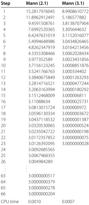
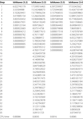
con-traction. In Tables -, we ﬁrst compare two cases of the Mann iteration method and also four cases of the Ishikawa and Agarwal iteration methods separately. From a mathematical point of view, one can see that the Mann iteration (.) is more than . times faster than the Mann iteration (.), the Ishikawa iteration (.) is more than . times faster than the Ishikawa iteration (.), the Ishikawa iteration (.) is more than . times faster than the Ishikawa iteration (.), the Ishikawa iteration (.) is more than  times faster

Table 1 Cases of Mann iteration

Step Mann (2.1) Mann (3.1)

1 15.2817976045 8.9908610772 2 11.8962912491 5.186577882 3 9.4591508761 3.8138707904 4 7.6992520365 3.305644632 5 6.4247631019 3.1152016077 6 5.4994648986 3.0434826465 7 4.8262347919 3.0164213456 8 4.3355308466 3.0062028434 9 3.977352589 3.0023431856 10 3.7156123245 3.0008851876 11 3.5241766763 3.000334402 12 3.3840675849 3.0001263293 13 3.2814716521 3.0000477244 14 3.2063163994 3.0000180292 15 3.1512468009 3.000006811 16 3.11088634 3.0000025731 17 3.0813015724 3.000000972 18 3.0596130334 3.0000003672 19 3.0437118532 3.0000001387 20 3.0320530065 3.0000000524 21 3.0235042722 3.0000000198 22 3.0172357852 3.0000000075 23 3.0126392095 3.0000000028 24 3.0092685565

25 3.0067968355 26 3.004984289

. . .

63 3.0000000517 64 3.0000000379 65 3.0000000278 66 3.0000000204

(19)

Table 2 Cases of Ishikawa iteration

Step Ishikawa (3.2) Ishikawa (3.3) Ishikawa (3.5) Ishikawa (3.4)

1 6.022745179 17.599516463 6.397259957 17.53342562 2 3.55504988 15.542488073 3.725044385 15.426710149 3 3.102829451 13.778956254 3.157958555 13.626959863 4 3.019085154 12.266356345 3.034584416 12.089125019 5 3.003543432 10.968408676 3.007580568 10.774826445 6 3.000657931 9.854176549 3.001661995 9.651358665 7 3.000122164 8.89726621 3.000364402 8.690843013 8 3.000022683 8.07514758 3.000079898 7.86950815 9 3.000004212 7.368577613 3.000017518 7.167078769 10 3.000000782 6.76111087 3.000003841 6.566256169 11 3.000000145 6.23868412 3.000000842 6.052276815 12 3.000000027 5.789263769 3.000000185 5.612537089 13 3.000000005 5.402546543 3.00000004 5.23627424 14 3.000000001 5.069705312 3.000000009 4.91429501

15 4.783173147 3.000000002 4.638744748

16 4.536459758 4.402910896

17 4.323995342 4.201055645

18 4.14099766 4.028273397

19 3.983358785 3.880369278

20 3.847548529 3.753755571

21 3.730532022 3.645363373

22 3.629699305 3.55256722

23 3.542805134 3.473120743

24 3.467917475 3.405101727

25 3.403373393 3.346865184

26 3.347741258 3.297003256

27 3.299788327 3.254310946

28 3.258452935 3.217756821

29 3.222820611 3.18645797

30 3.192103569 3.159658578

31 3.165623078 3.136711605

32 3.142794307 3.117063114

33 3.123113286 3.100238856

34 3.1061457 3.0858328

35 3.09151723 3.07349731

CPU time 0.00086 0.0035 0.0016 0.0085

Table 3 Cases of Agarwal iteration

Step Agarwal (3.13) Agarwal (3.14) Agarwal (3.16) Agarwal (3.15)

1 3.663643981 4.231276342 4.038158759 4.165185499 2 3.034148064 3.125898552 3.08652991 3.112771857 3 3.001785887 3.013368608 3.007415671 3.011314821 4 3.000093479 3.001425297 3.000637055 3.001139398 5 3.000004893 3.000152024 3.000054738 3.000114779 6 3.000000256 3.000016216 3.000004703 3.000011563 7 3.000000013 3.00000173 3.000000404 3.000001165 8 3.000000001 3.000000184 3.000000035 3.000000117

9 3 3.00000002 3.000000003 3.000000012

10 3.000000002 3 3.000000001

11 3 3

(20)

Figure 1 CPU time.

than the Ishikawa iteration (.), the Ishikawa iteration (.) is more than . times faster than the Ishikawa iteration (.), the Agarwal iteration (.) is . times faster than the Agarwal iteration (.), the Agarwal iteration (.) is . times faster than the Agarwal iteration (.), the Agarwal iteration (.) is . times faster than the Agarwal itera-tion (.) and so on. We first add our CPU time in Tables - for each iteraitera-tion method. Also, we provide Figure  by using at least  times calculating of CPU times for our faster cases in the methods. From a computer-calculation point of view, we get a different an-swer. As one can see in the CPU time table, we found that the Agarwal iteration (.) and the Mann iteration (.) are faster than the Ishikawa iteration (.). This note emphasizes the difference of the mathematical results and computer-calculation results which have appeared many times in the literature.

The next example illustrates Lemma ..

Example  LetX=R,C= [, ],x= ,αn= .,βn= ., andγn= . for all

n≥. Deﬁne the mapT:C→Cby the formulaT(x) =√x_{for all}_x_∈_{C. Table  shows} us that the Abbas iteration (.) converges faster than the other cases, the Abbas iteration (.) is . times faster than the Abbas iteration (.), the Abbas iteration (.) is . times faster than the Abbas iteration (.), the Abbas iteration (.) is . times faster than the Abbas iteration (.) and . times faster than the Abbas iteration (.) and the Abbas iteration (.). One can get similar results about diﬀerence of the mathematical and computer-calculating points of views for this example.

The next example illustrates Theorem ..

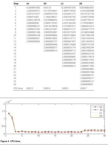
Example  LetX=R,C= [, ],x= ,αn= .,βn= ., andγn= . for alln≥.

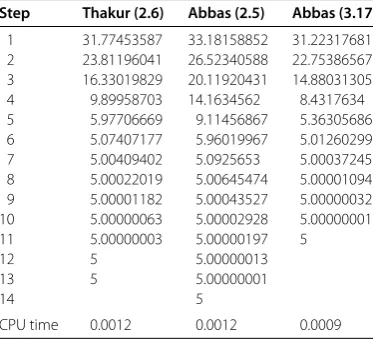
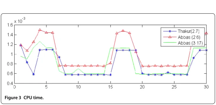
Deﬁne the mapT:C→CbyT(x) =√x_{– x}_{+  for all}_x∈_C_{(see []). Table  shows} the Abbas iteration (.) converges . times faster than the Thakur-Thakur-Postolache iteration (.) and the Thakur-Thakur-Postolache iteration (.) is . times faster than the Abbas iteration (.) from the mathematical point of view. Again, we get diﬀerent results from the computer-calculating point of view by checking Table  and Figures  and .

(21)

Table 4 Cases of Abbas iteration

Step Abbas (3.17) Abbas (3.18) Abbas (3.19) Abbas (3.20) Abbas (3.21) Abbas (3.22) Abbas (3.23) Abbas (3.24)

1 20.933947 23.074444 29.706456 30.294581 42.622758 43.000492 74.725586 74.829373 2 3.501533 3.915728 4.912771 5.052334 6.872931 6.975246 14.057893 14.097781 3 1.650123 1.789347 2.07514 2.127569 2.605814 2.644699 4.919453 4.938021 4 1.218545 1.278689 1.392374 1.417334 1.596596 1.615195 2.581994 2.592232 5 1.080705 1.109014 1.161005 1.174049 1.254442 1.264388 1.750749 1.757015 6 1.030883 1.044439 1.069469 1.076461 1.115609 1.121158 1.389425 1.39348 7 1.011982 1.018426 1.030642 1.034379 1.054109 1.057231 1.212285 1.214975 8 1.004673 1.007695 1.013649 1.015622 1.025684 1.02743 1.119022 1.120821 9 1.001827 1.003223 1.006106 1.007132 1.012273 1.013239 1.067815 1.069015 10 1.000715 1.001351 1.002737 1.003264 1.005884 1.006411 1.038999 1.039794 11 1.00028 1.000567 1.001228 1.001495 1.002825 1.00311 1.022548 1.02307 12 1.000109 1.000238 1.000551 1.000685 1.001357 1.00151 1.013078 1.013417 13 1.000043 1.0001 1.000247 1.000314 1.000653 1.000733 1.007599 1.007818 14 1.000017 1.000042 1.000111 1.000144 1.000314 1.000356 1.00442 1.00456 15 1.000007 1.000018 1.00005 1.000066 1.000151 1.000173 1.002572 1.002661 16 1.000003 1.000007 1.000022 1.00003 1.000073 1.000084 1.001498 1.001554 17 1.000001 1.000003 1.00001 1.000014 1.000035 1.000041 1.000872 1.000907 18 1.000001 1.000005 1.000006 1.000017 1.00002 1.000508 1.00053 19 1.000001 1.000002 1.000003 1.000008 1.00001 1.000296 1.00031 20 1 1.000001 1.000001 1.000004 1.000005 1.000172 1.000181

21 1 1 1.000001 1.000002 1.000002 1.0001 1.000106

22 1 1 1 1.000001 1.000001 1.000058 1.000062

23 1 1 1 1 1.000001 1.000034 1.000036

24 1 1 1 1 1.00002 1.000021

25 1 1 1 1.000012 1.000012

26 1 1 1 1.000007 1.000007

27 1 1 1.000004 1.000004

28 1 1 1.000002 1.000002

29 1 1 1.000001 1.000001

30 1.000001 1.000001

31 1 1

32 1 1

33 1 1

34 1 1

35 1 1

36 1 1

37 1 1

Table 5 Comparison between Thakur iteration and Abbas iteration

Step Thakur (2.6) Abbas (2.5) Abbas (3.17)

1 31.77453587 33.18158852 31.22317681 2 23.81196041 26.52340588 22.75386567 3 16.33019829 20.11920431 14.88031305 4 9.89958703 14.1634562 8.4317634 5 5.97706669 9.11456867 5.36305686 6 5.07407177 5.96019967 5.01260299 7 5.00409402 5.0925653 5.00037245 8 5.00022019 5.00645474 5.00001094 9 5.00001182 5.00043527 5.00000032 10 5.00000063 5.00002928 5.00000001 11 5.00000003 5.00000197 5

12 5 5.00000013

13 5 5.00000001

14 5

(22)

Figure 2 Convergence behavior of the iteration methods of Thakur equation (2.6), Abbas equation (2.5), and Abbas equation (3.17).

Example  LetX=R,C= [, ], andx= . Deﬁne the mapT: R→Rby T(x) =

x

 +  for allx∈C. Consider the following coeﬃcients separately in the Thakur-Thakur-Postolache iteration (.):

(a) αn=βn=γn=  –₍_n_+),

(b) αn=βn=γn=  –_n_+,

(c) αn=βn=γn=  – 

(n+)

,

(d) αn=βn=γn=  – 

(n+)

(23)

Table 6 Cases of Thakur iteration

Step (a) (b) (c) (d)

1 4.2609841803 9.03125 10.2844561595 10.8540663001 2 2.2826469537 4.2135416667 5.4804739263 6.2632682688 3 2.0353310377 2.6009419759 3.3595601275 4.0142167756 4 2.004416382 2.1466298421 2.5007642765 2.9360724936 5 2.0005520478 2.0330086855 2.1756764587 2.4287794141 6 2.000069006 2.0069770545 2.0591364356 2.1939030837 7 2.0000086257 2.0014018838 2.0192087915 2.0866824323 8 2.0000010782 2.0002701847 2.0060472121 2.0383477219 9 2.0000001348 2.0000502881 2.0018515929 2.0168034488 10 2.0000000168 2.0000090866 2.0005529869 2.0072985299 11 2.0000000021 2.0000016005 2.0001614712 2.0031443476 12 2.0000000003 2.0000002757 2.0000461907 2.0013443922

13 2.0000000466 2.0000129668 2.0005707329

14 2.0000000077 2.0000035774 2.0002406784

15 2.0000000013 2.0000009712 2.0001008564

16 2.0000002597 2.0000420126

17 2.0000000685 2.0000174019

18 2.0000000178 2.0000071693

19 2.0000000046 2.0000029385

20 2.0000000012 2.0000011985

21 2.0000004865

22 2.0000001966

23 2.0000000791

24 2.0000000317

25 2.0000000127

26 2.000000005

CPU time 0.0013 0.0014 0.0015 0.0017

Competing interests

The authors declare that they have no competing interests.

Authors’ contributions

All authors contributed equally to this work. All authors read and approved the ﬁnal manuscript.

Author details

1_{Department of Mathematics, Azarbaijan Shahid Madani University, Tabriz, Iran.}2_{Department of Mathematics and}

Informatics, University Politehnica of Bucharest, Bucharest, 060042, Romania.

Acknowledgements

The basic idea of this work has been given to the fourth author by Professor Mihai Postolache during his visit to University Politehnica of Bucharest in September 2014. The ﬁrst and fourth authors was supported by Azarbaijan Shahid Madani University.

(24)

References

1. Plunkett, R: On the rate of convergence of relaxation methods. Q. Appl. Math.10, 263-266 (1952) 2. Bowden, BV: Faster than Thought: A Symposium on Digital Computing Machines. Pitman, London (1953) 3. Byrne, C: A uniﬁed treatment of some iterative algorithms in signal processing and image reconstruction. Inverse

Probl.20(1), 103-120 (2004)

4. Dykstra, R, Kochar, S, Robertson, T: Testing whether one risk progresses faster than the other in a competing risks problem. Stat. Decis.14(3), 209-222 (1996)

5. Hajela, D: On faster than Nyquist signaling: computing the minimum distance. J. Approx. Theory63(1), 108-120 (1990)

6. Hajela, D: On faster than Nyquist signaling: further estimations on the minimum distance. SIAM J. Appl. Math.52(3), 900-907 (1992)

7. Longpre, L, Young, P: Cook reducibility is faster than Karp reducibility in NP. J. Comput. Syst. Sci.41(3), 389-401 (1990) 8. Shore, GM: Faster than light: photons in gravitational ﬁelds - causality, anomalies and horizons. Nucl. Phys. B460(2),

379-394 (1996)

9. Shore, GM: Faster than light: photons in gravitational ﬁelds. II. Dispersion and vacuum polarisation. Nucl. Phys. B 633(1-2), 271-294 (2002)

10. Stark, RH: Rates of convergence in numerical solution of the diﬀusion equation. J. Assoc. Comput. Mach.3, 29-40 (1956)

11. Argyros, IK: Iterations converging faster than Newton’s method to the solutions of nonlinear equations in Banach space. Ann. Univ. Sci. Bp. Rolando Eötvös Nomin., Sect. Comput.11, 97-104 (1991)

12. Argyros, IK: Suﬃcient conditions for constructing methods faster than Newton’s. Appl. Math. Comput.93, 169-181 (1998)

13. Lucet, Y: Faster than the fast Legendre transform: the linear-time Legendre transform. Numer. Algorithms16(2), 171-185 (1997)

14. Berinde, V: Picard iteration converges faster than Mann iteration for a class of quasi-contractive operators. Fixed Point Theory Appl.2004(2), 97-105 (2004)

15. Berinde, V, Berinde, M: The fastest Krasnoselskij iteration for approximating ﬁxed points of strictly pseudo-contractive mappings. Carpath. J. Math.21(1-2), 13-20 (2005)

16. Berinde, V: A convergence theorem for Mann iteration in the class of Zamﬁrescu operators. An. Univ. Vest. Timi¸s., Ser. Mat.-Inform.45(1), 33-41 (2007)

17. Babu, GVR, Vara Prasad, KNVV: Mann iteration converges faster than Ishikawa iteration for the class of Zamﬁrescu operators. Fixed Point Theory Appl.2006, Article ID 49615 (2006)

18. Popescu, O: Picard iteration converges faster than Mann iteration for a class of quasi-contractive operators. Math. Commun.12(2), 195-202 (2007)

19. Akbulut, S, Ozdemir, M: Picard iteration converges faster than Noor iteration for a class of quasi-contractive operators. Chiang Mai J. Sci.39(4), 688-692 (2012)

20. Gorsoy, F, Karakaya, V: A Picard S-hybrid type iteration method for solving a diﬀerential equation with retarded argument (2014). arXiv:1403.2546v2 [math.FA]

21. Hussain, N, Chugh, R, Kumar, V, Raﬁq, A: On the rate of convergence of Kirk-type iterative schemes. J. Appl. Math. 2012, Article ID 526503 (2012)

22. Ozturk Celikler, F: Convergence analysis for a modiﬁed SP iterative method. Sci. World J.2014, Article ID 840504 (2014)

23. Thakur, D, Thakur, BS, Postolache, M: New iteration scheme for numerical reckoning ﬁxed points of nonexpansive mappings. J. Inequal. Appl.2014, 328 (2014)

24. Berinde, V: Iterative Approximation of Fixed Points. Springer, Berlin (2007)

25. Chugh, R, Kumar, S: On the rate of convergence of some new modiﬁed iterative schemes. Am. J. Comput. Math.3, 270-290 (2013)

26. Mann, WR: Mean value methods in iteration. Proc. Am. Math. Soc.4, 506-510 (1953) 27. Ishikawa, S: Fixed points by a new iteration method. Proc. Am. Math. Soc.44, 147-150 (1974)

28. Noor, MA: New approximation schemes for general variational inequalities. J. Math. Anal. Appl.251, 217-229 (2000) 29. Agarwal, RP, O’Regan, D, Sahu, DR: Iterative construction of ﬁxed points of nearly asymptotically nonexpansive

mappings. J. Nonlinear Convex Anal.8(1), 61-79 (2007)