Nonparametric Bayesian sparse factor analysis for frequency domain blind source separation without permutation ambiguity

(1)

R E S E A R C H

Open Access

Nonparametric Bayesian sparse factor analysis

for frequency domain blind source separation

without permutation ambiguity

Kohei Nagira

*

, Takuma Otsuka and Hiroshi G Okuno

Abstract

Blind source separation (BSS) and sound activity detection (SAD) from a sound source mixture with minimum prior information are two major requirements for computational auditory scene analysis that recognizes auditory events in many environments. In daily environments, BSS suffers from many problems such as reverberation, a permutation problem in frequency-domain processing, and uncertainty about the number of sources in the observed mixture. While many conventional BSS methods resort to a cascaded combination of subprocesses, e.g., frequency-wise separation and permutation resolution, to overcome these problems, their outcomes may be affected by the worst subprocess. Our aim is to develop a unified framework to cope with these problems. Our method, called permutation-free infinite sparse factor analysis (PF-ISFA), is based on a nonparametric Bayesian framework that enables inference without a pre-determined number of sources. It solves BSS, SAD and the permutation problem at the same time. Our method has two key ideas: unified source activities for all the frequency bins and the activation probabilities of all the frequency bins of all the sources. Experiments were carried out to evaluate the separation performance and the SAD performance under four reverberant conditions. For separation performance in the BSS EVAL criteria, our method outperformed conventional complex ISFA under all conditions. For SAD performance, our method outperformed the conventional method by 5.9–0.5% inF-measure under the condition RT20=30–600 [ms], respectively.

1 Introduction

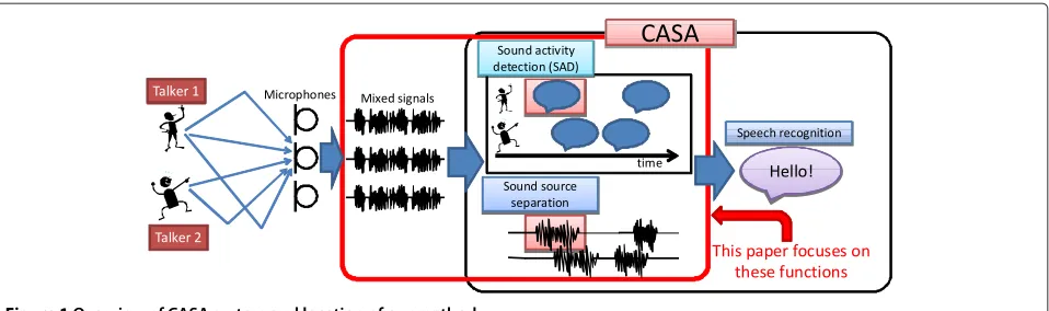
Computational auditory scene analysis (CASA) aims to ﬁnd auditory events and extract valuable information from captured sound signals [1,2]. An overview of CASA system is depicted in Figure 1. First, the CASA system cap-tures sound signals by using a microphone array. Then, it detects sound activities of each source and separates the mixture into individual sources. Finally, it visualizes the auditory events or recognizes these separated sound sources. This article focuses on the source activity detec-tion (SAD) and sound source separadetec-tion. SAD is useful for CASA systems because this function helps these systems discover audio sources especially when a huge amount of archived audio signals is analyzed. Another example of the beneﬁt of the SAD is compatibility with automatic speech recognition. For accurate automatic speech recognition, it is necessary to extract the voiced part, which is referred to

*Correspondence: [email protected]

Graduate School of Informatics, Kyoto University, Sakyo, Kyoto, Japan

as voice activity detection [3,4]. Sound source separation is essential for CASA systems because we often observe a mixture of multiple sound sources in our daily environ-ment. Our goal is to develop a simultaneous sound activity detection and sound source separation system for CASA.

The combination of sound source separation and source activity detection should overcome the following diﬃcul-ties for real-world applications:

1. unknown mixing processes, 2. source number uncertainty, 3. reverberation, and

4. performance degradation caused by mutually dependent functions.

The ﬁrst one indicates that the CASA system should work without information speciﬁc to a certain environment or a situation such as the environment’s impulse responses or the sound source locations. The second one expresses that the CASA system should achieve robust estimation under the condition that the number of sources is unknown. The

(2)

Figure 1Overview of CASA system and location of our method.

third one means that the mixture of audio signals cap-tured in a room may contain reverberations that affect the microphone array processing. The last one means that cascaded processing to cope with the above-mentioned difficulties may be severely affected by the worst subcess of the CASA system. When source separation pro-cessing is performed in the frequency domain, the output signals are affected by the permutation problem, which is ambiguity in the output order for different frequency bins. Conventional methods take the cascade approach. The mixed signals are separated for each frequency bin first, and then the permutation problem is solved. As men-tioned above, the overall performance is limited to the performance of the worst subprocess.

Our solution for overcoming these diﬃculties is as follows. The mixing process is modeled stochastically and inferred on the basis of this model. To handle source number uncertainty, we introduce a nonparamet-ric Bayesian approach. The reverberation is absorbed by using frequency-domain processing. Uniﬁed analysis of the source separation and permutation resolution is used to optimize these mutually dependent functions.

This article presents a permutation-free inﬁnite sparse factor analysis (PF-ISFA): a joint estimation method that simultaneously achieves frequency-domain source sepa-ration and SAD using a minimum amount of prior infor-mation. PF-ISFA achieves robust estimation without using prior information about the number of sources. PF-ISFA extends the frequency-domain ISFA [5], which is a non-parametric Bayesian frequency-domain source separation method. We build a generative process that explains the observed sound source mixture and derive a Bayesian inference to retrieve respective sound sources and sound activities. The key idea of PF-ISFA is that all the frequency bins of signals are processed at the same time to avoid the permutation problem. In particular, a uniﬁed source activ-ity for all frequency bins is introduced into its generative model.

The rest of this article is organized as follows. Section 2 summarizes the main problem treated, and introduces

study related to our method. Section 3 explains con-ventional ISFA in the time and frequency domains and then introduces our new method PF-ISFA. Section 4 gives detailed posterior inferences of PF-ISFA. Section 5 presents experimental results, and Section 6 concludes this article.

2 Problem statement and related study

This section starts by summarizing the problem that is solved in this article and the assumptions needed to solve it. After that, the study related to this problem, especially concerning source separation, the permutation problem, and sound detection methods, are introduced.

2.1 Problem statement

The problem statement is brieﬂy summarized below. Input:

• Sound mixtures ofK sources captured by D microphones.

Output:

• EstimatedK source signals,

• Detected source activities of source signals.

Assumptions:

1. The number of sourcesK is not more than the

number of microphonesD.

2. The locations of the sources do not change.

(3)

the mixing process from the sources to the microphones is unchanged.

2.2 Requirements

This system should fulﬁll some requirements in order to work in daily environments. These requirements are summarized as follows.

1. Blind source separation, 2. Frequency domain processing, 3. Permutation resolution,

4. Robust estimation without source knowledge, and 5. Uniﬁed approach.

These requirements are described in detail below.

2.2.1 Blind source separation

One of the system’s major requirements is to work with the minimum amount of prior information. This is because getting prior information, such as the direction of arrival of sound or the reverberation level of the room, in advance is a troublesome task for the system. In addi-tion, even if the prior information can be obtained, the separation performance is severely aﬀected by the quality of the information. The system should not be dependent on such information. The source separation method that uses the minimum prior information is called blind source separation (BSS).

2.2.2 Frequency domain processing

There are two reasons why frequency domain processing is inevitable for CASA. One is to deal with reverbera-tion and the other is to model source signals using the sparseness of sound energy.

The mixing process of speech signals in our daily sur-roundings is modeled as a convoluted mixture [6]. The signals captured by the microphones consist of a mixture of ones from various sources and they are contaminated by reﬂections, reverberations, and arrival time lags at the microphones. To model these time-delayed signals, a convoluted mixture is often used.

Attempts to solve a BSS problem involving convoluted mixtures of signals mainly use, frequency domain pro-cessing. This is because the convoluted mixture in the time domain can be explained in a simplistic form in the frequency domain. Speciﬁcally, the short time Fourier transform (STFT) can convert a convoluted mixture in the time domain into instantaneous mixtures for all frequency bins. In other words, STFT can absorb the reverberation of the source signals within the window length. Thus, fre-quency domain processing is eﬀective when BSS is applied to audio signals in practical situations.

2.2.3 Permutation resolution

As mentioned above, the convoluted mixture in the time domain is converted into instantaneous mixtures for

individual frequency bins. Many frequency-domain BSS methods independently separate the mixed signals for all the frequency bins; thus, an ambiguity arises in the out-put order. The system must arrange the separated signals in the correct order for the frequency bins. This is called the “permutation problem”. The permutation problem should be solved in order to achieve frequency-domain BSS.

2.2.4 Robust estimation without source knowledge

Many CASA systems and many source separation meth-ods use prior knowledge about source signals for robust estimation to improve the performance. For instance, HARK [7] localizes the sound sources before separa-tion by using the number of sources. When independent component analysis (ICA), a well-known BSS method, is applied to the input signals, principal component analy-sis (PCA) is commonly used as preprocessing for ICA [8]. This is because the number of dimensions of ICA’s input signals can be reduced. However, getting prior knowledge about sources is diﬃcult for the system, so robust estima-tion without source knowledge is desirable. A nonpara-metric Bayesian framework is helpful for robust inference without knowing the number of sources.

2.2.5 Uniﬁed approach

A unified estimation method enables effective process-ing because it makes the most of the information avail-able from the observed signals. Many source separation frameworks use a cascaded approach. For instance, HARK [7] localizes the sources first and then separates the observed signals into individual sources; the conventional frequency-domain ICA separates the observations and then resolves the permutation problem. One of the critical weak points of these cascaded approaches is that the sep-aration performance is limited to the performance of the worst subprocess.

2.3 Related study

2.3.1 Source separation method of speech signals

(4)

Many BSS methods have already been introduced. One well-known BSS method is ICA, which separates mixed signals on the basis of the statistical independence between of diﬀerent source signals. Many algorithms are used for ICA, such as the minimization mutual informa-tion [10], Fast ICA [11], and JADE [12]. For BSS for speech signals, frequency-domain ICA is commonly used [13]. While ICA does achieve BSS, it does not detect the activ-ities of individual sources; moreover, frequency-domain ICA is plagued by the permutation problem.

ISFA [14] is a BSS method based on the nonparametric Bayesian approach. It achieves SAD and BSS simulta-neously, but it is modeled in the time domain, so it is vulnerable to the reverberation that often appears in our daily surroundings.

Frequency-domain ISFA (FD-ISFA), which we proposed in our previous study [5], can handle a convoluted mixture that contains room reverberation. One problem for FD-ISFA is the permutation problem. Conventional FD-FD-ISFA independently separates the signals for all the frequency bins, so it cannot avoid permutation ambiguity.

2.3.2 Permutation problem

Some methods solve the permutation problem by post processing. One method is based on estimation of the direction of arrival and inter-frequency correlation of the signal envelopes [15]; another uses the power ratio of the signals as a dominance measure [16].

Other methods avoid this problem by using a uniﬁed criterion from among all frequency bins. Independent vector analysis (IVA) [17] and permutation-free ICA [18] are BSS methods that avoid the permutation problem. These methods are based on ICA and cannot simultane-ously achieve sound source detection.

2.3.3 BSS framework achieving SAD

Some BSS frameworks obtain SAD information simulta-neously. Switching ICA [19] is a BSS method which can achieve SAD. Switching ICA employs a hidden Markov model (HMM) on its model to represent whether the source is active or not. The SAD information is obtained from these estimated hidden variables of HMM. Non-stationary Bayesian ICA [20] achieves dynamic source separation by estimating the sources and the mixing matrices for each time frame on the basis of variational Bayesian inference. The SAD information is obtained from automatic relevance determination (ARD) parame-ters, which are the precision parameters of the probabilis-tic density of the mixing matrix. Since these methods are time-domain approaches, it is not appropriate for speech separation of convoluted mixtures.

The combination of a maximize signal-to-noise ratio beamformer, a voice activity detector and online cluster-ing achieves BSS and SAD [21]. This method is a cascade

approach. It achieves SAD and the time-diﬀerence of arrival estimation ﬁrst and then separates signals using this them. As mentioned above, the weak point of cas-caded approach is that the separation performance is limited to the performance of the worst subprocess.

3 ISFA

This section ﬁrst summarizes conventional methods for ISFA: Section 3.1 shows the model of ISFA in the time domain [14], and Section 3.2 explains its expansion into the frequency domain (FD-ISFA) [5] and its problems. Then, Section 3.3 describes a model of FD-ISFA without permutation ambiguity (PF-ISFA).

3.1 ISFA in time domain

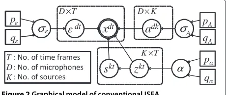
ISFA [14] achieves BSS of instantaneous mixtures of time-domain signals without knowing the number of sources. It is based on the following instantaneous mixture model, which expresses thatD×Tobserved dataXis composed of a linear combination ofK×Tsource signalsS.

X=A(ZS)+E, (1)

whereAis aD×K mixing matrix,Eis aD×T Gaus-sian noise term, andZis a binary mask onX.denotes element-wise multiplication. Letxdt,adk,zkt,skt,εdtbe the elements ofX,A, Z, S, andE, respectively. The genera-tive model of ISFA is shown in Figure 2.σ_A2andσ_ε2are the variance parameters of the elements ofAandE.

The priors of these parameters are as follows:

ε_t∼N(0,σ_ε2I), σ_ε2∼IG(pε,qε), (2)

skt∼N(0, 1), (3) ak ∼N(0,σA2I), σA2∼IG(pA,qA), and (4)

Z∼IBP(α), α∼G(pα,qα). (5)

Here,akis thekth row ofA, andpε,qε,pA,qA,pα, andqα are the hyperparameters. IBP(α)is the Indian buﬀet pro-cess (IBP) [22] with concentration parameterα. IBP [22] is a stochastic process that can deal with a potentially inﬁnite number of signals. It is used in order to achieve separa-tion without using prior knowledge about the number of sources.

x

dt

_a

dk

p

A

q

_A

z

kt

s

kt

T D×

A

σ

α

q

_α

p

_α

σ

ε

p

_ε

q

_ε

dt

ε

T K×

K D×

T D K

(5)

In the time domain, each element ofX,A,S, andEis a real-valued variable. Each of these variables has a normal distribution as a prior.N(μ,σ2)is a normal distribution with mean μ and variance σ2. The probability density function of this normal distribution is

N(x;μ,σ2) = √ 1

2π σ2exp

−(x−μ)2

2σ2

. (6)

The IBP concentration parameter has a gamma prior, and the variance parameters of A and E have inverse gamma priors. G(b,θ ) and IG(b,θ ) are gamma distri-bution and the inverse gamma distridistri-bution with shape parameter b and scale parameter θ, respectively. The probability density functions of these distributions are

G(x;b,θ ) = x b−1

(b) θbexp

−x θ

, and (7)

IG(x;b,θ ) = x −(b+1)

(b) θbexp

− 1

θx

. (8)

A Bayesian hierarchical model aims at explaining the uncertainty in the model from the observed data by treat-ing latent variables as a probabilistic variable rather than a ﬁxed value. In our model, we place a gamma prior on the concentration parameter of IBP so that the emergence of sources inZcan be controlled by the data we have.

3.2 ISFA in frequency domain

Since the convoluted mixture is converted into complex spectra by using STFT, the elements ofX, S, A, and E become complex-valued variables. FD-ISFA is a model for complex values that arises in frequency-domain process-ing. It can deal with an instantaneous mixture of complex spectra.

The generative model is the same as for time-domain ISFA. However, the priors of these complex-valued ele-ments are diﬀerent from those of time-domain ISFA.

ε_t ∼ N_C(0,σ_ε2I), (9) skt ∼ NC(0, 1), and (10)

ak ∼ NC(0,σA2I) (11)

Here, instead of the normal distribution, a univariate com-plex normal distributionNC is used for complex-valued

parameters. The probability density functions of this dis-tribution is

NC(x;μ,σ2)=

1

π σ2exp

−|x−μ|2 σ2

. (12)

Conjugacy is one of the helpful properties of Bayesian inference. If we choose a conjugate prior, a closed-form expression can be given for the posterior. The variances

σ_ε2 and σ_A2 have a conjugate inverse gamma prior, and the Gaussian conjugate prior can be used for the mixing matrixA. For simplicity, the univariate complex normal

distribution is introduced as a conjugate prior of source signal S. It is noted that a super-Gaussian prior, such as student-t or Laplace distribution, should be used for speech signals. The complex extension of these distri-butions is non-trivial. We don’t deal with the complex super-Gaussian prior in this article and this is one of our future study.

The processing ﬂow of FD-ISFA is as follows. After STFT, the complex spectra are whitened in each frequency bin, and FD-ISFA is applied for each frequency bin of these complex spectra independently. FD-ISFA is plagued by two well-known ambiguities of frequency domain BSS: the scaling ambiguity and permutation ambiguity. The scaling ambiguity is that the amplitude of the output sig-nals may not equal that of the original sources. Some post-processing methods are needed to resolve these two ambiguities. The projection back method [23] is an eﬀec-tive solution for the scaling ambiguity. The permutation ambiguity is solved by using the methods mentioned above [15,16]. After these problems have been solved, esti-mated complex spectra are assembled into source signals by using inverse STFT.

3.3 New method: PF-ISFA

Our new method, permutation-free ISFA (PF-ISFA), achieves both BSS and SAD without being affected by the permutation problem. Its key idea for avoiding the per-mutation problem is unified activity for each time frame. Conventional ISFA is applied independently to each fre-quency bin. That is to say, conventional ISFA does not consider any relations across frequency bins. This is the main reason for the permutation problem. By contrast, in the PF-ISFA model, all frequency bins are unified by the activity matrix. Since this unified activity controls the out-put order of source signals, PF-ISFA is not affected by the permutation problem.

The ﬂow of PF-ISFA is depicted in Figure 3, and the gen-erative process of PF-ISFA is described in Figure 4. LetF be the number of frequency bins. PF-ISFA is also based on instantaneous mixture for each frequency bin. PF-ISFA deals with the F-tuple frequency bins at the same time. The elements ofZ,X,S,E, andAare deﬁned asxfdt,afdk,

zfkt,sfkt,εfdt, respectively.

The following model is introduced to unify the activities of all frequency bins.

zfkt=bktφ, φ∼Bernoulli(ψkf), (13)

(6)

Figure 3Schematic overview for our method.

The prior distributions of the newly introduced variables are assumed to be as follows:

B ∼ IBP(α), α∼G(pα,qα), and (14)

∼ Beta

β

K,

β(K−1)

K

. (15)

PF-ISFA estimates the source signals S, their time-frequency activitiesZ, the mixing matrixA, uniﬁed activi-tiesB, activation probabilities, and other parameters by using only the observed signalX.

x

fdt

_a

fdk

fdt

p

q

p

q

p

_A

q

_A

z

fkt

s

fkt kf

b

kt

T D F× ×

σ

A

ψ

α α α

β ε

ε

T K× T K F× ×

F K×

K D F× ×

F T D K

Figure 4Graphical model of PF-ISFA.

One of the main differences between this PF-ISFA model and conventional ISFA model is the unified activity matrix for each time frameBand the activation probabil-ity matrix for each frequency bin . A graphical model of conventional ISFA is shown in Figure 2. Whereas each frequency bin is independently estimated in the conven-tional ISFA model, all frequency bins are bundled together by the unified activity matrix in the PF-ISFA model.

The likelihood function of PF-ISFA is written as follows.

P(X|A,S,Z) = F

f=1

T

t=1

P(xft|Af,sft,zft)

= F

f=1

T

t=1

NC(xft;Af(zftsft),σε2I)

= F

f=1 1

(π σ2

ε)TD

exp

−tr(E

H

f Ef) σ2

ε

, (16)

where

Ef =Xf −Af(Zf Sf). (17)

(7)

4 Inference of PF-ISFA

The model parameters of PF-ISFA are estimated by using an iterative algorithm based on the nonparamet-ric Bayesian model. Sound source separation and SAD are achieved by estimatingskft andbkt, respectively. The parameter update algorithm is given as follows.

1. Initialize parameters using their priors. 2. At each timet, carry out the following:

2-1 For each sourcek, samplebktfrom Equation (26).

2-2 Ifbkt=1, samplezkftfrom Equation (20) and for each frequency binf ; otherwisezkft =0. 2-3 Ifzkft=1, sampleskftfrom Equation (18);

otherwiseskft=0.

2-4 Determine the number of new classesκt, and initialize the parameters.

3. For each sourcek and frequency bin f, sample the activation probabilityψkffrom Equation (28). 4. For each sourcek and frequency bin f, sample mixing

matrixakffrom Equation (29).

5. If there is a source that is always inactive, remove it. 6. Updateσ_ε2,σ_A2, andαfrom Equations (30), (31), and

(32), respectively. 7. Go to 2.

This method is based on the Metropolis-Hastings algo-rithm [24]. The posterior distributions of the latent vari-ables are derived from Bayes’ theorem by multiplying the priors by the likelihood function.

4.1 Sound sources

Whenzfktis active,sfktis sampled by using the following posterior.

P(sfkt|Af,s−fkt,xftzft) ∝ P(xft|Af,sft,zft,σε2)P(sfkt)

= NC

sfkt;μs,f,σs2,f

, (18)

where

σ_s2_,_f = σ

2 ε

σ2

ε +aHfkafk

, μ_s_,_f = a

H fkε−fkt

σ2

ε +aHfkafk .

Here, s−fkt means sft except for sfkt, and ε−fkt means

ε|_z_fkt₌₀.

4.2 Source activity of each time-frequency frame

Ifbkt = 1,zfktis sampled from its posterior distribution. The posterior ofzfktis calculated as follows.

P(zfkt|bkt,ψkf,z−fkt,xft,sft,Af) ∝ PpPl (19)

where

Pl=P(xft|Af,sft,zft,σε2)

is the probability of likelihood, and

Pp=P(zfkt|bkt,ψkf)

is the probability of prior.

Then, the following posterior distribution is derived.

P(zfkt|bkt,ψkf,z−fkt,xft,sft,Af)=Bernoulli

p1 p0+p1

,

(20)

where

log(p1)=log(ψkf)+

2Re(s∗_fktaH_kfε₋_fkt)+ |sfkt|2aHfkafk

σ2

ε

(21)

log(p0)=log(1−ψkf). (22)

4.3 Uniﬁed activity for each time frame

To calculate the ratio of the probability thatbktbecomes active to the probability thatbktbecomes inactive,we use Equation (23). This ratioris divided into two parts: the ratio of prior rp and the ratio of the likelihood of fth

frequency binrl,f.

r = P(bkt=1|A,S−kt,Xt,S−kt) P(bkt=0|A,S−kt,Xt,Z−kt)

= rp F

f=1

rl,f, (23)

where

rp =

P(bkt=1|bkt) P(bkt=0|bkt)

, and

rl,f =

P(xft|Af,s−fkt,xft,z−fkt,b−kt,bkt=1,ψkf,σε2)

.

Here, Xt isx1t,. . .,xFt and S−kt and Z−kt are S and Z except fors1kt,. . .,sFktandz1kt,. . .,zFkt, respectively.

The ratio of priorrpis calculated by using:

rp=

P(bkt=1|b−kt) P(bkt=0|b−kt) =

mk,−t

T−mk,−t

, (24)

wheremk,−t = t=tbkt. This is derived from the priors

of source activity based on IBP [22].

The ratio of likelihood rl,f is calculated by using

Equation (25).

rl,f =

= ψ_kfσ_s2_,_fexp

|μ_s_,_f|2 σ_s2_,_f

(8)

Figure 5Microphone array for measuring impulse response.

The posterior probability ofzkt = 1 is calculated using ratior.

P(bkt=1|A,S−kt,Xt,Z−kt,b−kt)= r

1+r (26)

To decide whether or notbktis active, we sampleufrom Uniform(0,1) and compare it with r/(1 + r). If u ≤ r/(1+r), thenbktbecomes active; otherwise, it remains dormant.

4.4 Number of new sources

Some source signals that were not active at the beginning are active at timetfor the ﬁrst time. Letκ_tbe the number of these sources. Thisκ_tis sampled with the Metropolis-Hastings algorithm.

First, the prior distribution of κ_t is P(κ_t|α) =

Poisson_Tα. After sampling κt, we initialize the new

sources and their activities. Next, we decide whether this update is acceptable or not. Letξ andξ∗ be the current state (i.e., the condition before transition) and the next state candidate (the condition after transition), respec-tively. The acceptance probability of the transition is min(1,rξ→ξ∗). According to Meeds [25] and Knowles [14], rξ→ξ∗ becomes the ratio of the likelihood of the current state to that of the next state. This ratio can be calculated as follows.

rξ→ξ∗ =

F

f=1

(detξ,f)−1exp

μH_ξ_,_fξ,fμξ,f

, (27)

where

ξ,f =I+

A∗_fHA∗_f

σ2

ε

,ξ,fμξ,f =

1

σ2

ε

A∗_fHε_ft.

Here,A∗_f is theD×κtmatrix of the additional part ofAf.

When newκtsources appear, the mixing matrix should be

expanded fromD×KtoD×(K+κt).A∗_f means the mixing

matrix for these new sources.

4.5 Activation probability for each frequency bin ψ_kfis sampled by the following posterior.

P(ψ_kf|zkf,−kf,B−kt)∝P(ψkf|β)

T

t=1

P(zkft|ψkf,bkt)

=Beta

β

K +nkf,

β(K−1)

K +mk−nkf

,(28)

where nkf = Tt=1zkft is the number of active time-frequency frames of sourcekin thefth frequency bin, and mk = Tt=1bkt is the number of active time frames of sourcek.

4.6 Mixing matrix

The mixing matrix is estimated in each column. The posterior distribution is

P(afk|Af,−k,Sf,Xf,Zf) ∝P(Xf|Af,Sf,Zf,σε2)P(afk|σA2) =NC(afk;μA,−A1), (29)

where

A=

sH_fksfk

σ2

ε

+ 1

σ_A2

ID,μA=

σ_A2

sH_fksfkσA2+σε2

Ef|akf=0sfk.

4.7 Variance of noise and mixing matrix

The variance of noise corresponds to the noise level of the estimated signals, and the variance of the mixing matrix aﬀects the scale of the estimated signals. Their posteriors are as follows.

P(σ_ε2|E)∝P(E|σ_ε2)P(σ_ε2|pε,qε)

=IG

σ_ε2;pε+FTD,

qε

(1+qε F_f₌₁tr(EH_f Ef))

.

(9)

Table 1 Experimental conditions

No. of sourcesK 2

Sampling rate 16 [kHz]

STFT window length 64 [ms]

STFT shift length 32 [ms]

Iterations 300 [times]

Hyperparameters (pε,qε)=(10000, 1.0)

(pA,qA)=(1.1, 0.1) (pα,qα)=(3.2, 0.21)

β=0.5

P(σ_A2|A)∝P(A|σ_A2)P(σ_A2|pA,qbfA)

=IG

σ_A2;pA+FDK,

qA

1+qA Ff=1tr(AHf Af)

(31)

4.8 Concentration parameter of IBP

The posterior distribution of concentration parameterαis

p(α|B) ∝ P(B|α)P(α|pα,qα)

= G

α;K++pα, qα 1+qαHT

, (32)

where K₊ is the active number of sources, and Hn = n

j=11j is thenth harmonic number.

5 Experimental results

In this section, we evaluate the separation performance and the accuracy of the source activity. Section 5.1 presents the results of separation performance and SAD performance compared with FD-ISFA [5]. Section 5.2 shows the separation results compared with PF-ICA [18] using two or four microphones (D = 2, 4) and various source locations.

Figure 6Locations of microphones and sources of Section 5.1.

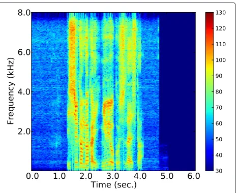
Figure 7Spectrogram of source signal.

5.1 Compared with FD-ISFA

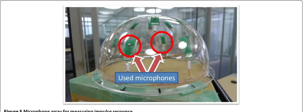
The experiments used simulated mixtures in four rooms with reverberation times of 20, 150, 400, and 600 [ms]. The simulated mixtures were generated by convoluting the impulse responses measured in the rooms. These impulse responses were recorded by using the microphone array depicted in Figure 5. We use two microphones in these experiments (D = 2). The microphone and source loca-tions are shown in Figure 6, and experimental condiloca-tions are listed in Table 1. For each condition, 200 mixtures using JNAS phoneme-balanced sentences were tested.

The values of these hyperparameters are empirically-selected. The smallσ_ε2means the smaller the noise term becomes. Therefore, pε and qε is set to 10000 and 1.0

in order to get smaller variance. In contrast, σ_A2 should have a certain amount becauseσ_A2aﬀects the amplitudes

(10)

Figure 9Spectrogram of FD-ISFA separated signal.

of output signals. If σ_A2 is too large, the power of esti-mated signals become small, and then these signals are considered to be inactive.

5.1.1 Separation performance

First, an example of the experimental results obtained from the separation experiment using mixed signals (D= 2) in a room with reverberation time of 20 [ms] is shown. Spectrograms of a source signal, a signal separated using PF-ISFA, a signal separated using conventional FD-ISFA, and a permutation-aligned signal separated using FD-ISFA are shown in Figures 7, 8, 9, and 10, respectively.

When FD-ISFA is used, the results, shown in Figure 9, contained many horizontal lines; however, there are fewer of these lines in Figure 10. These lines are the spectrogram

Figure 10Spectrogram of permutation-aligned FD-ISFA separated signal.

Table 2 Separation result of Section 5.1 [dB]

RT20=20ms

PF-ISFA FD-ISFA

Perm Non-perm Perm Solver

SDR 10.07 8.21 12.95 7.94

ISR 17.44 14.71 19.28 13.22

SIR 19.86 16.81 20.30 13.99

SAR 11.70 11.13 15.40 14.48

RT20=150ms

SDR 6.85 4.71 6.68 4.21

ISR 11.62 9.30 11.33 8.35

SIR 11.16 8.15 10.84 7.24

SAR 11.38 10.15 11.32 10.62

RT20=400ms

SDR 5.22 3.14 6.53 3.00

ISR 9.97 7.70 10.95 7.26

SIR 9.81 6.93 10.73 6.53

SAR 9.49 8.68 11.77 10.77

RT20=600ms

SDR 3.57 1.56 4.26 1.16

ISR 8.07 5.89 8.67 5.37

SIR 7.01 4.07 7.72 3.37

SAR 8.21 7.73 9.19 8.41

(11)

Table 3 Average SAD performance: precision, recall, andF-measure

Precision (%) Recall (%) F-measure (%)

RT20 FD-ISFA PF-ISFA FD-ISFA PF-ISFA FD-ISFA PF-ISFA

20 [ms] 64.9 77.6 88.8 84.6 74.1 80.0

150 [ms] 67.6 69.2 93.5 92.9 77.5 78.4

400 [ms] 68.7 75.1 89.5 84.3 76.9 78.6

600 [ms] 71.7 75.2 90.7 87.1 79.3 79.8

of the other separated signal. This means that the output orders of the FD-ISFA results are not aligned for all fre-quency bins. However, there are no horizontal lines in the spectrogram of PF-ISFA (Figure 8). This shows that the output order is aligned; in other words, the permutation problem has been solved by using PF-ISFA.

The spectrogram shown in Figure 8 has vivid time structure. This indicates that the constraint on the uni-ﬁed activity is too strong and the activation probability for each frequency bin becomes almost one. In order to improve this phenomenon, we might introduce a hyper-parameter which can control the activation probability appropriate to observed signals.

We also evaluated our method in terms of the signal-to-distortion ratio (SDR), the image-to-spatial distortion ratio (ISR), the source-to-interference ratio (SIR), and the source-to-artifacts ratio (SAR) [26]. SDR is an overall measure of the separation performance; ISR is a measure of the correctness of the inter-channel information; SIR is

a measure of the suppression of the interference signals; and SAR is a measure of the naturalness of the separated signals.

The results are summarized in Table 2. Larger value means better separation. “Non-Perm” was calculated from the output signals themselves; in other words, their mutations were not aligned. “Solver” means that the per-mutations were aligned using inter-frequency correlation of signal envelope. “Perm” means that the output signals permutations are aligned using the correlation between the outputs and the original sources; in other words, the permutations were aligned by using the original source signals for reference.

Our method (PF-ISFA) outperformed FD-ISFA with permutation solver for all criteria except for SAR under all conditions. In particular, it improved the SIR by 2.82 dB under the condition RT20 = 30 [ms], 0.91 dB under RT20 = 150 [ms], 0.41 dB under RT20 = 400 [ms], and 0.70 dB under RT20=600 [ms].

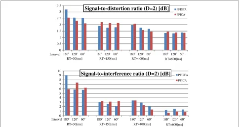
0 0.5 1 1.5 2 2.5 3 3.5

180 120 60 180 120 60 180 120 60 180 120 60

Signal-to-distortion ratio (D=2) [dB]

PFISFA PFICA

RT=30[ms] RT=150[ms] RT=400[ms] RT=600[ms] Interval

0 1 2 3 4 5 6 7 8 9 10

180 120 60 180 120 60 180 120 60 180 120 60

Signal-to-interference ratio (D=2) [dB]

PFISFA PFICA

(12)

One of the reasons of the poor performance of FD-ISFA is due to the cascade approach. The results show that FD-ISFA achieves better performance if the permutation problem is perfectly solved. Therefore, this poor perfor-mance comes from the permutation solver. This indi-cates that the overall performance of cascade approach is severely aﬀected by the performance of worst subprocess. These results show that the performance in rooms with reverberation times of 150, 400, and 600 [ms] is worse than for RT20 = 30 [ms] reverberation. This is because the reverberation time of these rooms are longer than the STFT window length (64 [ms]). If the reverberation time is longer than the STFT window length, the reverbera-tion aﬀects multiple time frames, and this degrades the performance.

The result of PF-ISFA (Perm) and that of PF-ISFA (Non-Perm) is different. If the source activity results are poor, the activities of two separated signals become similar. In this case, the permutation ambiguity is likely to arise because the unified activity matrix becomes meaningless. In other words, PF-ISFA marks better result when each source signal has different activity.

5.1.2 SAD performance

Next, we evaluated our method in SAD accuracy. The SAD result of PF-ISFA was estimated as uniﬁed source activities, that is the parameter bft in Section 3.3. Since FD-ISFA estimated the sound activity for each frequency bin independently, we calculated the number of active

bins for each time frame and determined the source activ-ity of each time frame by using threshold processing.

The precision rate, recall rate, and F-measure of the source activity accuracy are listed in Table 3. PF-ISFA results are indicated by bold type. PF-ISFA outperformed FD-ISFA in precision rate andF-measure in all reverber-ant conditions. In particular, it improved theF-measure by 5.9 points, 0.9 points, 1.7 points, and 0.5 points under the conditions RT20 = 30 [ms], 150 [ms], 400 [ms], and 600 [ms], respectively.

Our method achieved a better precision rate and lower recall rate than FD-ISFA, and the results show that PF-ISFA achieved robust SAD performance under reverber-ant condition. This is because PF-ISFA estimates the source activities using a uniﬁed parameter for all fre-quency bins. PF-ISFA is less likely to determine that the time frame is active, even if some frequency bins have a certain power level.

5.2 Compared with PF-ICA

In second experiment, we used two or four microphones (D= 2, 4) to observe the two sound source mixture with interval θ = 60, 120, and180[deg]. For each interval, 20 mixtures were tested using JNAS phoneme-balanced sen-tences. The microphone and source locations is shown in Figure 11. We use red microphones whenD=2. In order to calculate SDR, ISR, SIR, and SAR, two signals which maximize SDR score are chosen from estimated signals when using four microphones.

0 0.5 1 1.5 2 2.5 3 3.5

180 120 60 180 120 60 180 120 60 180 120 60

Signal-to-distortion ratio (D=4) [dB]

PFISFA PFICA

0 2 4 6 8 10 12 14

180 120 60 180 120 60 180 120 60 180 120 60

Signal-to-interference ratio (D=4) [dB]

_PFISFA

PFICA

(13)

Table 4 Separation result of Section 5.2 [dB]

RT20=20ms

D=2 D=4

PF-ISFA PF-ICA PF-ISFA PF-ICA

SDR 2.76 2.32 1.95 2.51

ISR 3.53 3.54 2.36 3.27

SIR 6.87 6.48 9.90 6.87

SAR 7.39 9.96 5.61 11.28

RT20=150ms

D=2 D=4

SDR 1.82 2.15 1.28 3.01

ISR 2.71 3.02 1.64 3.34

SIR 2.64 3.19 5.50 11.45

SAR 6.37 7.67 3.58 9.55

RT20=400ms

D=2 D=4

SDR 1.79 1.71 1.57 1.95

ISR 2.80 2.93 1.96 2.69

SIR 2.84 2.35 6.31 4.60

SAR 6.56 9.37 4.46 9.62

RT20=600ms

D=2 D=4

SDR 1.36 1.40 1.19 1.51

ISR 2.38 2.52 1.59 2.22

SIR 1.36 0.79 4.40 3.50

SAR 5.81 9.41 3.69 8.55

The average SDR and SIR of separated signals are shown in Figures 12 and 13 for each interval whenD=2 and 4, respectively. Table 4 summarizes average SDR, ISR, SIR, and SAR of all intervals.

Table 4 indicates that PF-ISFA marks better average SIR except for the condition RT20 = 150 [ms]. This means that PF-ISFA can suppress the interference signal better than PFICA. PF-ISFA and PF-ICA marks similar results by the average SDR whenD = 2, and The SDR score of PF-ISFA is lower than that of PF-ICA whenD=4. This is because these SDR scores are aﬀected by the SAR scores. The output signals of PF-ICA are created by multiplying separation matrix by observed signals. Then, the artiﬁcial noise is not likely to emerge. In contrast, PF-ISFA esti-mates the source signals by sampling, and PF-ISFA output is based on the best one sample of all samples created during estimation.

6 Conclusion and future study

This article presented a joint estimation method of BSS and SAD in the frequency domain that also solves the permutation problem. It was designed by using a non-parametric Bayesian approach. Uniﬁed source activity was introduced to automatically align the permutations of the output order for all frequency bins.

Our method improves the average SIR by 2.82–0.41 dB compared with the baseline method based on FD-ISFA when separating convoluted mixtures of RT20 = 30 [ms]–600 [ms] room environments. It also outper-forms FD-ISFA under reverberant conditions (RT20 = 150, 400, 600 ms). For SAD performance, our method out-performs the conventional method by 5.9–0.5% in F-measure under the condition RT20 = 20–600 [ms], respectively.

In the future, we will evaluate the separation perfor-mance of a mixture of signals from three or more talkers. We will attempt to develop a method that can separate mixtures with longer reverberations (i.e., longer than the STFT window length) robustly. Last but not least, the method should be sped up to achieve real-time processing so that it can be applied to robot applications.

Competing interests

The authors declare that they have no competing interests.

Acknowledgements

This study was partially supported by KAKENHI and Honda Research Institute Japan Inc., Ltd.

Received: 16 June 2012 Accepted: 27 October 2012 Published: 22 January 2013

References

1. D Rosenthal, HG Okuno,Computational auditory scene analysis(CRC press, USA, 1998)

2. D Wang, G Brown,Computational auditory scene analysis: principles, algorithms, and applications(Wiley-IEEE press, USA, 2006)

3. J Sohn, N Kim, W Sung, A statistical model-based voice activity detection. IEEE Signal Process. Lett.6, 1–3 (1999)

4. J Ramırez, J Segura, C Benıtez, A De La Torre, A Rubio, Eﬃcient voice activity detection algorithms using long-term speech information. Speech Commun.42(3), 271–287 (2004)

5. K Nagira, T Takahashi, T Ogata, HG Okuno, inProc. of International Conference on Latent Variable Analysis and Signal Separation. Complex extension of inﬁnite sparse factor analysis for blind speech separation, Tel-Aviv, 2012), pp. 388–396

6. MS Pedersen, J Larsen, U Kjems, LC Parra, inSpringer Handbook of Speech Processing, ed. by J Benesty, MM Sondhi, and Y Huang. Convolutive blind source separation methods, Part I (Springer Press, 2008), pp. 1065–1094 7. K Nakadai, T Takahashi, H Okuno, H Nakajima, Y Hasegawa, H Tsujino,

Design and implementation of robot audition system “HARK” open source software for listening to three simultaneous speakers. Adv. Robot. 24(5), 739–761 (2010)

8. F Asano, S Ikeda, M Ogawa, H Asoh, N Kitawaki, Combined approach of array processing and independent component analysis for blind separation of acoustic signals. IEEE Trans. Speech Audio Process.11(3), 204–215 (2003)

(14)

parameter control for real-world blind source separation, Las Vegas, 2008), pp. 149–152

10. P Comon, Independent component analysis, a new concept? Signal Process.36(3), 287–314 (1994)

11. A Hyv¨arinen, Fast and robust ﬁxed-point algorithms for independent component analysis. IEEE Trans. Neural Netw.10(3), 626–634 (1999) 12. J Cardoso, A Souloumiac, Blind beamforming for non-Gaussian signals.

IEE Proceedings F Radar and Signal Processing.140(6), 362–370 (1993) 13. H Sawada, R Mukai, S Araki, S Makino, inProc. of IEEE International

Conference on Acoustics, Speech, and Signal Processing. Polar coordinate based nonlinear function for frequency-domain blind source separation, Orlando, 2002), pp. 1001–1004

14. D Knowles, Z Ghahramani, inProc. of Independent Component Analysis and Signal Separation. Inﬁnite sparse factor analysis and inﬁnite independent components analysis, London, 2007), pp. 381–388

15. H Sawada, R Mukai, S Araki, S Makino, A robust and precise method for solving the permutation problem of frequency-domain blind source separation. IEEE Trans. Speech Audio Process.12(5), 530–538 (2004) 16. H Sawada, S Araki, S Makino, inProc. of IEEE International Symposium on

Circuits and Systems. Measuring dependence of bin-wise separated signals for permutation alignment in frequency-domain BSS, New Orleans, 2007), pp. 3247–3250

17. I Lee, T Kim, T Lee, Fast ﬁxed-point independent vector analysis algorithms for convolutive blind source separation. Signal Process.87(8), 1859–1871 (2007)

18. A Hiroe, inProc. of International Conference on Independent Component Analysis and Blind Signal Separation. Solution of permutation problem in frequency domain ICA, using multivariate probability density functions, Charleston, 2006), pp. 601–608

19. J Hirayama, S Maeda, S Ishii, Markov and semi-Markov switching of source appearances for nonstationary independent component analysis. IEEE Trans. Neural Netw.18(5), 1326–1342 (2007)

20. H Hsieh, J Chien, inProc. of IEEE International Conference on Acoustics Speech and Signal Processing. Online Bayesian learning for dynamic source separation, Dallas, 2010), pp. 1950–1953

21. S Araki, H Sawada, S Makino, inProc. of IEEE International Conference on Acoustics, Speech and Signal Processing, vol. 1. Blind speech separation in a meeting situation with maximum SNR beamformers, Honolulu, 2007), pp. 41–44

22. T Griffiths, Z Ghahramani, Infinite latent feature models and the Indian buffet process. Adv. Neural Inf. Process. Syst.18, 475–482 (2006) 23. N Murata, S Ikeda, A Ziehe, An approach to blind source separation based

on temporal structure of speech signals. Neurocomputing.41, 1–24 (2001)

24. W Hastings, Monte Carlo sampling methods using Markov chains and their applications. Biometrika.57(1), 97–109 (1970)

25. E Meeds, Z Ghahramani, R Neal, S Roweis, Modeling dyadic data with binary latent factors. Adv. Neural Inf. Process. Syst.19, 977–984 (2007) 26. E Vincent, H Sawada, P Boﬁll, S Makino, J Rosca, inProc. of Independent Component Analysis and Signal Separation. First stereo audio source separation evaluation campaign: data, algorithms and results, London, 2007), pp. 552–559

doi:10.1186/1687-4722-2013-4

Cite this article as:Nagiraet al.:Nonparametric Bayesian sparse factor analysis for frequency domain blind source separation without permuta-tion ambiguity.EURASIP Journal on Audio, Speech, and Music Processing2013

2013:4.