R E S E A R C H
Open Access
A generalized groundwater flow equation
using the concept of variable-order derivative
Abdon Atangana
*and Joseph Francois Botha
*Correspondence:
[email protected] Institute for Groundwater Studies, Faculty of Natural and Agricultural Sciences, University of the Free State, P.O. Box 9301, Bloemfontein, South Africa
Abstract
In this paper, the groundwater flow equation is generalized using the concept of the variational order derivative. We present a numerical solution of the modified groundwater flow equation with the variational order derivative. We solve the generalized equation with the Crank-Nicholson technique. Numerical methods typically yield approximate solutions to the governing equation through the discretization of space and time and can relax the rigid idealized conditions of analytical models or lumped-parameter models. They can therefore be more realistic and flexible for simulating field conditions. Within the discredited problem domain, the variable internal properties, boundaries, and stresses of the system are
approximated. We perform the stability and convergence analysis of the Crank-Nicholson method and complete the paper with some illustrative computational examples and their simulations.
Keywords: groundwater flow equation; variable order derivative; Crank-Nicholson scheme; stability; convergence
1 Introduction
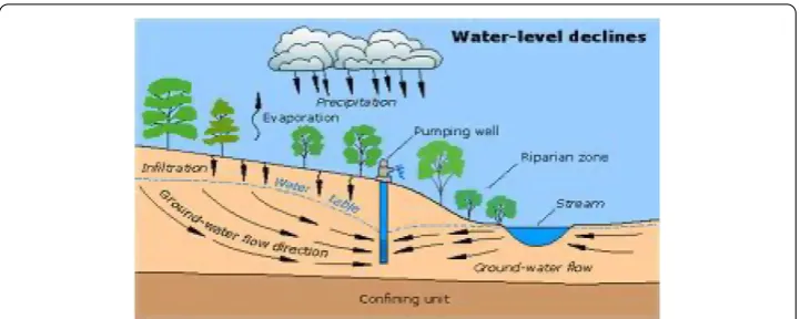
A problem that arises naturally in groundwater investigations is to choose an appropri-ate geometry for the geological system in which the flow occurs. This geological forma-tion, through which the groundwater flows, changes in time and space. Figure shows the groundwater flow direction toward the pumping well during the extraction of water from the aquifer. The main effort is to establish a suitable mathematical relation between different observables, or what [] calls a mathematical model for the observables. An ideal mathematical model should not merely provide links between different observables, but also lead to a better understanding of the phenomenon. The attractiveness of this approach is that the mathematical model could, in principle, be used to investigate the future be-havior of a given phenomenon under various conditions. This leads us to the groundwater flow equation. This model is based on the conventional, saturated groundwater flow equa-tion for density-independent flow:
S(x,t)∂t(x,t) =∇ ·[K∇] +f(x,t). (.)
HereSis the specific storativity,Kis the hydraulic conductivity tensor of the aquifer,
Figure 1 Groundwater flow in the borehole during pumping test.
derivation of Eq. (.), we will show the Darcy law
q(x,t) =K(x,t) (.)
is used as a keystone in the derivation of Eq. (.). This law, proposed by Darcy early in the nineteenth century, relies on experimental results obtained from the flow of water through a one-dimensional sand column. Alternatively, Darcy’s law states that the rate of flow through a porous medium is proportional to the loss of head and inversely propor-tional to the length of the flow path. Note that the specific dischargeq(x,t) has the dimen-sions of velocity. Recent investigations [] suggest that the flow is also influenced by the geometry of the bedding parallel fractures, the feature that equation (.) cannot account for. It is therefore possible that equation (.) may not be applicable to the flow in these fractured aquifers. In an attempt to circumvent this problem, Barker [] introduced the model in which the geometry of the aquifer is regarded as a fractal. Although this model has been applied with reasonable success in the analysis of hydraulic tests from boreholes in Karoo aquifers [], it introduces parameters for which no sound definition exists in the case of non-integer flow dimensions. Recently [, ], the concept of a fractional-order derivative was used to generalize the groundwater flow equation. However, it has been found that the constant-order fractional diffusion equations are not capable of character-izing some complex diffusion processes, for instance, diffusion process in aninhomoge-neous or heterogeaninhomoge-neous medium [].
2 Modified groundwater flow equation
For the readers that are not acquainted with the concept of the variational order derivative, we start this section by presenting the basic definition of this derivative.
2.1 Variational order differential operator
Letf :R→R,x→f(x) denote a continuous and necessary differentiable, letα(x) be a continuous function in (, ]. Then its variational order differential in [a,∞) is defined as
Dα(x)f(x)=
( –α(x))
x
(x–t)–α(t)df(t)
dt dt. (.)
The above derivative is called the Caputo variational order differential operator; in addi-tion, the derivative of the constant is zero.
2.2 Problem formulation
Groundwater models describe the groundwater flow and transport processes using math-ematical equations based on certain simplifying assumptions. These assumptions typically involve the direction of flow, geometry of the aquifer, the heterogeneity or anisotropy of sediments or bedrock within the aquifer. This geological formation, through which the groundwater flows, changes in time and space.
The simplest generalization of the groundwater flow equation, which incidentally is also in accord with true physics of the phenomenon, is to assume that water level is not in a steady but transient state. Theis () [] was the first to develop a formula for unsteady-state flow that introduces the time factor and the storativity. He noted that when a well penetrating an extensive confined aquifer is pumped at a constant rate, the influence of the discharge extends outward with time. The rate of decline of head multiplied by the storativity and summed over the area of influence equals the discharge. The unsteady-state (or Theis) equation, which was derived from the analogy between the flow of groundwater and the conduction of heat, is perhaps the most widely used partial differential equation in groundwater investigations
SDt(r,t) =TDrr(r,t) +
rDr(r,t). (.)
The above equation is classified under a parabolic equation. To include explicitly the vari-ability of the medium through which the flow takes place, the standard version of the partial derivative with respect to time is replaced here with variable-order (VO) fractional to obtain
⎧ ⎨ ⎩
SDαt(x,t)(r,t) =TDrr(r,t) +rDr(r,t),
<α(x,t)≤. (.)
3 Numerical solution
Numerical methods yield approximate solutions to the governing equation through the discretization of space and time. Within the discredited problem domain, the variable in-ternal properties, boundaries, and stresses of the system are approximated. Determinis-tic, distributed-parameter, numerical models can relax the rigid idealized conditions of analytical models or lumped-parameter models, and they can therefore be more realistic and flexible for simulating field conditions. The finite difference schemes for constant-order time or space fractional diffusion equations have been widely studied [–]. For constant-order time fractional diffusion equations, Chenet al.proposed an implicit dif-ference approximation scheme []. Yusteet al.introduced weighted average finite differ-ence methods []. Podlubnyet al.proposed the matrix approach for fractional diffusion equations [], and Hanert proposed a flexible numerical scheme for the discretization of the space-time fractional diffusion equation []. Recently, Zhuanget al.considered the numerical schemes for VO space fractional advection-dispersion equation [], Linet al.
investigated the explicit scheme for VO nonlinear space fractional diffusion equation []. Before applying the numerical methods, we assume Eq. (.) has a unique and sufficiently smooth solution. To establish the numerical schemes for the above equation, we letxl=lh,
≤l≤M,Mh=L,tk=kτ, ≤k≤N,Nτ=T,his the step andτ is the time size,Mand Nare grid points.
3.1 Crank-Nicholson scheme [24]
We introduce the Crank-Nicholson scheme as follows. Firstly, the discretization of first-and second-order space derivative is stated as follows:
∂ ∂r =
(rl+,tk+) –(rl–,tk+)
(h)
+
(rl+,tk) –(rl–,tk)
(h)
+O(h), (.)
∂
∂r =
(rl+,tk+) – (rl,tk+) +(rl–,tk+)
(h)
+
(rl+,tk) – (rl,tk) +(rl–,tk)
(h)
+Oh, (.)
=
(rl,tk+) +(rl,tk)
. (.)
The Crank-Nicholson scheme for the VO time fractional groundwater flow model can be stated as follows:
∂αkl+(rl,tk+)
∂tαkl+
= τ
–αkl+
( –αk+l )
(rl,tk+) –(rl,tk)
+
k
j=
(rl,tk+–j) –(rl,tk–j)
(j+ )–αkl+– (j)–αkl+
. (.)
Now, replacing equations (.), (.), (.) and (.) in (.), we obtain the following:
Sτ–αkl+
( –αlk+)
(rl,tk+) –(rl,tk)
+
k
j=
(rl,tk+–j) –(rl,tk–j)
(j+ )–αkl+– (j)–αlk+
=T
(rl+,tk+) – (rl,tk+) +(rl–,tk+)
(h)
+
(rl+,tk) – (rl,tk) +(rl–,tk)
(h)
+ rl
(rl+,tk+) –(rl–,tk+)
(h)
+
(rl+,tk) –(rl–,tk)
(h)
.
For simplicity, let us put:
bl,k+j = (j+ )–αkl+– (j)–αkl+; Tk+ l =
( –αlk+)ταkl+ Sh T;
Gk+l =( –α
k+ l )τ
αkl+
Sh and λ
l,k+ j =b
l,k+ j– –b
l,k+ j .
(.)
Equation (.) becomes
k+l + Tlk+=k+l+
Tlk++G
k+ l rl
+k+l–
Tlk+–G
k+ l rl
+kl+
Tlk+–G
k+ l rl
+k+l + Tlk+
+
k
j=
k+–jl –k–jl λl,k+j Glk+. (.)
4 Stability analysis of the Crank-Nicholson scheme
In this section, we will analyze the stability conditions of the Crank-Nicholson scheme for the generalized groundwater flow equation.
Letζk
l =kl– kl. Here kl is the approximate solution at the point (xl,tk) (k= , , . . . ,N, l= , , . . . ,M– ) and, in addition,ζk= [ζk
,ζk, . . . ,ζM–k ]Tand the functionζk(x) is chosen
to be
ζk(x) = ⎧ ⎨ ⎩
ζlk ifxl–h <x≤xl+h,l= , , . . . ,M– ,
ifL–h<x≤L. (.)
Then the functionζk(x) can be expressed in Fourier series as follows:
ζk(x) =
m=∞
m=–∞
δm(m)exp[iπmk/L],
δk(x) =
L
L
ρk(x)exp
iπmx
L
dx.
(.)
It was established by Chenet al.[] that
ρ
= m=∞
m=–∞
δk(m). (.)
of the coefficientsTlk+,Glk+,λl,k+j , andbk+l can be established: . Gk+l ,Tlk+ are positive for alll= , , . . . ,M– ;
. <λl,kj ≤λl,kj–≤ for alll= , , . . . ,M– ; . ≤bl,kj ≤,
k–
j=
bl,k+j+ = –λl,k+k for alll= , , . . . ,M– .
(.)
It is customary in groundwater investigations to choose a point on the centerline of the pumped borehole as a reference for the observations, and therefore neither the drawdown nor its derivatives will vanish at the origin, as required. In such situations where the dis-tribution of the piezometric head in the aquifer is a decreasing function of the distance from the borehole, the expression
rl →. Under this situation, the error committed while
approximating the solution of the generalized groundwater flow equation with the Crank-Nicholson scheme can be presented as follows:
ζlk+ + Tlk+=ζl+k+Tlk++ζl–k+Tlk++ζl+k Tlk++ζlk + Tlk+
+
k
j=
ζlk+–j–ζlk–jλl,k+j Gk+l . (.a)
If we assume thatζlkin equation (.) can be put in the delta-exponential form as follows:
ζlk=δkexp[iφlk], (.b)
whereφis a real spatial wave number, new replacing the above equation (.b) into (.a), we obtain
+ Tlsin
φh
δ=
– Tlsin
φh
δ fork= ,
+ Tl+ksin
φh
δk+=
– Tl+ksin
φh
–λl,k+
δk (.)
+
k–
j=
λl,k+j+ δk–j+λl,k+k δ fork= , , . . . ,N– .
Equation (.) can be written in the following form:
δ=
[ – T l sin
(φh )]δ
[ + T l sin(
φh )]
,
δk+=
[ – Tl+ksin(φh) –el,k+ ]δk+
k–
j=λ l,k+
j+ δk–j+λl,k+k δ
[ + Tl+ksin(φh)] .
(.)
Our next concern here is to show that for allk= , , . . . ,N– , the solution of equation (.) satisfies the following condition:
|δk|<|δ|.
Fork= and remembering thatdk+l ,bk+l are positive for alll= , , . . . ,M– , we obtain
|δ|
|δ|
=[ – T
l sin
(φh )]
[ + T lsin
(φh )]
< . (.)
Assuming that form= , , . . . ,kthe property is verified, we get
|δk+|=
[ – Tl+ksin(
φh ) –e
l,k+ ]δk+
k–
j=λ l,k+
j+ δk–j+λl,k+k δ
[ + Tl+ksin(φh)]
. (.)
Making use of the triangular inequality we obtain
|δk+| ≤
| – Tl+ksin(φh) –el,k+ ||δk|+|
k–
j=p l,k+
j+ δk–j|+|el,k+k δ|
| + Tl+ksin(φh)| . (.)
Using the recurrence hypothesis, we have
|δk+| ≤
| – T+k l sin
(φh )|+|
k–
j=λ l,k+ j+ |
| + T+k l sin
(φh )|
|δ|,
|δk+| ≤
|
+ Tl+ksin(φh)| | + Tl+ksin(φh)|
|δ|, (.)
|δk+|<|δ|,
which this completes the proof.
5 Convergence analysis of the Crank-Nicholson scheme
If we assume that(rl,tk) (l= , , . . . ,M,k= , , . . . ,N– ) is the exact solution of our
problem at the point (rl,tk), by lettinglk=(rl,tk) –kl andk= (,k,k, . . . ,kM–),
substituting this in equation (.), we obtain
ζl + Tl–ζl+ Tl–ζl– Tl=Rl fork= ,
ζl+k + Tl+k–ζl+k+Tl+k–ζl–+kTl+l=R+kl +
k–
j=
k–jl λl,k+j+ fork≥.
(.)
Here,
R+kl =(rl,tk+) – k–
j=
(rl,tk–j)λl,k+j+ +b l,k+ (rl,t)
–Tl+k(rl+,tk+) – (rl,tk+) +(rl–,tk+)
. (.)
From equations (.) and (.), we have
∂(rl,tk+)
∂r +h V
=
((rl+,tk+) – (rl,tk+) +(rl–,tk+)) h
+((rl+,tk) – (rl,tk) +(rl–,tk))
h
∂αkl+(rl,tk+)
∂tαkl+
+τV
= τ
–αlk+
( –αk+l )
(rl,tk+) –(rl,tk) + k
j=
(rl,tk+–j) –(rl,tk–j)
λl,kj
.
From the above, we have that
Rk+l ≤Kτ+αlk++hταlk, (.)
whereK,K, andKare constants. Taking into account the Caputo-type fractional
deriva-tive, the detailed error analysis on the above schemes can refer to the work by Diethelm
et al.[] and further work by Li and Tao [].
Lemma k+∞≤K(τ+αlk++hταkl)(l,k+
j )–is true for(k= , , , . . . ,N– ),where
wk∞=max≤l≤M–(k),K is a constant.In addition,
αk+= ⎧ ⎨ ⎩
min≤l≤M–αlk+, ifτ< , max≤l≤M–αlk+, ifτ> .
This can be achieved via the recurrence technique on the natural number k.
Whenk= , we have the following:
l≤cl+blwl++cl– blwl–
=Fl≤Vτ+αkl++hτα k lλl,k+
j
–
. (.)
Now suppose thati+∞≤K(τ+αli++hταli)(λl,i+
j )–,i= , . . . ,N– . Then
w+kl ≤bk+l wk+l+ – wk+l +wk+l–+ck+l wk+l+ –wk+l–+dlk+wk+l
≤bk+l +ck+l wk+l++bk+l –ck+l wk+l–+dlk+– bk+l wk+l
= Rk+l +
k
i=
k–il λl,k+j
≤Rk+l +
k
i=
k–il λl,k+j
(.)
≤Kτ+αlk++hτα k l+
k
i=
k–il ∞λl,k+j
≤Kτ+αlk++hταklλl,k+ j +λ
l,k+ –λ
l,k+ j
λl,k+j –
≤Vτ+αkl++hταlkλl,k+
λl,k+j –
+kl ≤Vτ+αkl++hτα k lλl,k+
j
–
,
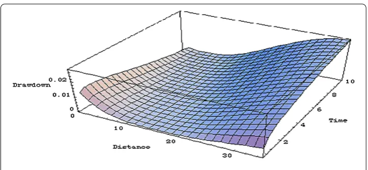
Figure 2 Drawdown as a function of space and time.
Theorem The Crank-Nicholson scheme is convergent,and there exists a positive constant V such that
kl–(xl,tk)≤K
τ+h, l= , , . . . ,M– ,k= , , . . . ,N. (.)
An interested reader can find the solvability of the Crank-Nicholson scheme in the work done by []. Therefore, the details of the proof will not be presented in this pa-per.
6 Numerical results
An image is worth ten thousand words; therefore, we devote this section to the nu-merical simulations of the solution of the generalized groundwater flow equation. The parameters used in the simulation are given as S= .,T = ,r∈[., ], and
t∈[, ].
Example
⎧ ⎪ ⎪ ⎨ ⎪ ⎪ ⎩
SDαt(x,t)(r,t) =TDrr(r,t) +rDr(r,t),
α(x,t) = –sin(rt),
(r, ) = .
(.)
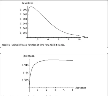
The numerical simulations of the approximate solution are presented in figures. First, Figure shows the solution as a function of time and space. Figure shows the solution as a function of time for a fixed distance. Figure shows the solution as a function of space for fixed time.
7 Conclusion
Figure 3 Drawdown as a function of time for a fixed distance.
Figure 4 Drawdown as a function of space for fixed time.
Competing interests
The authors declare that they have no competing interests.
Authors’ contributions
AA wrote the first draft and FJB corrected the final version. Both authors read and approved the final draft.
Acknowledgements
Dedicated to Professor Hari M Srivastava.
The authors would like to thank the referee for some valuable comments and helpful suggestions. This study was supported by the National Research Fund of South Africa.
Received: 30 January 2013 Accepted: 23 February 2013 Published: 14 March 2013
References
1. Botha, JF, Buys, J, Verwey, JP, Tredoux, G, Moodie, JW, Hodgkiss, M: Modelling groundwater contamination in the Atlantis aquifer. WRC Report No 175/1/90. Water Research Commission, P.O. Box 824, Pretoria 0001 (2004) 2. Van Tonder, GJ, Botha, JF, Chiang, WH, Kunstmann, H, Xu, Y: Estimation of sustainable yields of boreholes in fractured
rock formations. J. Hydrol.241, 70-90 (2001)
3. Barker, JA: A generalised radial flow model for hydraulic tests in fractured rock. Water Resour. Res.24(10), 1796-1804 (1988)
4. Van Der Voort, I: Risk-based decision tools for managing and protecting groundwater resources. PhD dissertation, University of the Free State, P.O. Box 339, Bloemfontein (2001)
5. Atangana, A: Numerical solution of space-time fractional order derivative of groundwater flow equation. In: International Conference of Algebra and Applied Analysis, Istanbul, June 20-24, p. 20 (2012)
6. Botha, JF, Cloot, AH: A generalized groundwater flow equation using the concept of non-integer order. Water SA
32(1), 1-7 (2006)
7. Solomon, TH, Weeks, ER, Swinney, HL: Observation of anomalous diffusion and Lévy flights in a two-dimensional rotating flow. Phys. Rev. Lett.71, 3975-3978 (1993)
8. Magin, RL, Abdullah, O, Baleanu, D, Zhou, XJ: Anomalous diffusion expressed through fractional order differential operators in the Bloch-Torrey equation. J. Magn. Reson.190, 255-270 (2008)
9. Sun, HG, Chen, W, Chen, YQ: Variable order fractional differential operators in anomalous diffusion modeling. Phys. A
388, 4586-4592 (2009)
10. Umarov, S, Steinberg, S: Variable order differential equations and diffusion with changing modes. Z. Anal. Anwend.
11. Ross, B, Samko, SG: Fractional integration operator of variable order in the Hölder spaceHλ(x). Int. J. Math. Math. Sci.
18, 777-788 (1995)
12. Chen, YQ, Moore, KL: Discretization schemes for fractional-order differentiators and integrators. IEEE Trans. Circ. Syst. I: Fund. Theoret. Appl.49, 363-367 (2002)
13. Theis, CV: The relation between the lowering of the piezometric surface and the rate and duration of discharge of a well using groundwater storage. Trans. Am. Geophys. Union16, 519-524 (1935)
14. Zhang, Y: A finite difference method for fractional partial differential equation. Appl. Math. Comput.215, 524-529 (2009)
15. Tadjeran, C, Meerschaert, MM, Scheffler, HP: A second order accurate numerical approximation for the fractional diffusion equation. J. Comput. Phys.213, 205-213 (2006)
16. Meerschaert, MM, Tadjeran, C: Finite difference approximations for fractional advection dispersion equations. J. Comput. Appl. Math.172, 65-77 (2004)
17. Deng, WH: Numerical algorithm for the time fractional Fokker-Planck equation. J. Comput. Phys.227, 1510-1522 (2007)
18. Li, CP, Chen, A, Ye, JJ: Numerical approaches to fractional calculus and fractional ordinary differential equation. J. Comput. Phys.230, 3352-3368 (2011)
19. Chen, CM, Liu, F, Turner, I, Anh, V: A Fourier method for the fractional diffusion equation describing sub-diffusion. J. Comput. Phys.227, 886-897 (2007)
20. Yuste, SB, Acedo, L: An explicit finite difference method and a new Von Neumann-type stability analysis for fractional diffusion equations. SIAM J. Numer. Anal.42, 1862-1874 (2005)
21. Podlubny, I, Chechkin, A, Skovranek, T, Chen, YQ, Vinagre Jara, BM: Matrix approach to discrete fractional calculus II: partial fractional differential equations. J. Comput. Phys.228, 3137-3153 (2009)
22. Hanert, E: On the numerical solution of space time fractional diffusion models. Comput. Fluids46, 33-39 (2011) 23. Lin, R, Liu, F, Anh, V, Turner, I: Stability and convergence of a new explicit finite-difference approximation for the
variable-order nonlinear fractional diffusion equation. Appl. Math. Comput.212, 435-445 (2009)
24. Crank, J, Nicolson, P: A practical method for numerical evaluation of solutions of partial differential equations of the heat conduction type. Proc. Camb. Philol. Soc.43(1), 50-67 (1947)
25. Diethelm, K, Ford, NJ, Freed, AD: Detailed error analysis for a fractional Adams method. Numer. Algorithms36, 31-52 (2004)
26. Li, CP, Tao, CX: On the fractional Adams method. Comput. Math. Appl.58, 1573-1588 (2009) doi:10.1186/1687-2770-2013-53