www.geosci-model-dev.net/7/1641/2014/ doi:10.5194/gmd-7-1641-2014
© Author(s) 2014. CC Attribution 3.0 License.
Influence of high-resolution surface databases on the modeling of
local atmospheric circulation systems
L. M. S. Paiva1, G. C. R. Bodstein2, and L. C. G. Pimentel2 1Federal Center of Technological Education, Rio de Janeiro, Brazil 2Federal University of Rio de Janeiro, Rio de Janeiro, Brazil
Correspondence to: G. C. R. Bodstein ([email protected])
Received: 16 October 2013 – Published in Geosci. Model Dev. Discuss.: 16 December 2013 Revised: 12 May 2014 – Accepted: 30 June 2014 – Published: 14 August 2014
Abstract. Large-eddy simulations are performed using the Advanced Regional Prediction System (ARPS) code at hor-izontal grid resolutions as fine as 300 m to assess the influ-ence of detailed and updated surface databases on the mod-eling of local atmospheric circulation systems of urban ar-eas with complex terrain. Applications to air pollution and wind energy are sought. These databases are comprised of 3 arc-sec topographic data from the Shuttle Radar Topogra-phy Mission, 10 arc-sec vegetation-type data from the Euro-pean Space Agency (ESA) GlobCover project, and 30 arc-sec leaf area index and fraction of absorbed photosynthetically active radiation data from the ESA GlobCarbon project. Sim-ulations are carried out for the metropolitan area of Rio de Janeiro using six one-way nested-grid domains that allow the choice of distinct parametric models and vertical resolutions associated to each grid. ARPS is initialized using the Global Forecasting System with 0.5◦-resolution data from the Na-tional Center of Environmental Prediction, which is also used every 3 h as lateral boundary condition. Topographic shading is turned on and two soil layers are used to compute the soil temperature and moisture budgets in all runs. Results for two simulated runs covering three periods of time are compared to surface and upper-air observational data to explore the de-pendence of the simulations on initial and boundary condi-tions, grid resolution, topographic and land-use databases. Our comparisons show overall good agreement between sim-ulated and observational data, mainly for the potential tem-perature and the wind speed fields, and clearly indicate that the use of high-resolution databases improves significantly our ability to predict the local atmospheric circulation.
1 Introduction
ARPS allows significant refinement of the numerical grid to the point where LES (large eddy simulation) can be used, since some turbulent parametric models developed for LES are available in the code. We chose the LES-ARPS model as our main tool because it is based on a 1.5 order of magni-tude turbulent kinetic energy (1.5-TKE) scheme and the Mo-eng and Wyngaard (1989) turbulence model and because it has been thoroughly tested (Chow, 2004; Chow et al., 2006) and used as a reference for the assessment of state-of-the-art mesoscale models such as WRF (Gasperoni, 2013). Among all turbulence parameterization schemes available in ARPS, the 1.5-TKE scheme and the Moeng and Wyngaard (1989) turbulence model is the best for this type of simulation. ARPS was formulated to be run in either a RANS (Reynolds-Averaged Navier–Stokes) or a LES code that solves the three-dimensional, compressible, nonhydrostatic, filtered Navier– Stokes equations. The relevant settings for our application requires the use of ARPS in the LES mode because the length scale is based on the grid spacing, as explained by Chow et al. (2006), and the difference between RANS and LES in this case is in the definition of the length scale (Michioka and Chow, 2008). For the LES mode, the length scale em-ployed in the eddy viscosity equation is based on the grid size, whereas the length scale for the RANS mode is based on a PBL (planetary boundary layer) depth or distance from the ground. The differences between RANS and LES become small when similar space and time resolutions are used in nu-merical modeling. This is also one of the four concepts rated by Pope (2000) that characterize the LES model, indicating that the physical and numerical modeling must be deliber-ately combined. Additionally, we prefer the LES procedure for our study because it is clear which physical features are resolvable and which must be modeled.
Several numerical studies available in the literature have adopted significant refinement of the grid in mesoscale sim-ulations. As an example, we may cite the simulations car-ried out by Grell et al. (2000), who used MM5 to compute the atmospheric flow in some regions of the Swiss Alps with horizontal resolutions of up to 1 km. It is worth noting that previous works, such as Lu and Turco (1995), point out that the increase in the spatial resolution of the grid can gener-ate more detailed and reliable solutions. In fact, most studies show that high-resolution numerical grids tend to improve the quality of numerically simulated data when compared to observed data (Revell et al., 1996; Grøn˙as and Sandvik, 1999; Grell et al., 2000; Chow et al., 2006). However, in re-gions of steep and extensive slopes, the topography may be poorly represented because the ramps that form the slopes on the surface may become irregular as the grid resolution is increased. In this case, the coarse spatial resolution of the topographic database does not add any additional informa-tion to the simulainforma-tions, since fine numerical grids require extensive surface information. The same concerns are ex-pressed in Chow (2004). Usually, high-resolution numeri-cal grids are often employed for simulations of small areas
due to the high computational cost. Revell et al. (1996) and Grøn˙as and Sandvik (1999) used numerical grids with reso-lutions of 250 m to perform LES simulations, but the wind field was not reproduced accurately in the regions studied. The authors considered that the main source of inaccuracy was the absence of high-resolution surface data. However, Zhong and Fast (2003) were successful in capturing the gen-eral characteristics of the surface fluxes present in the Salt Lake valley, in the state of Utah, using three of the mesoscale models cited above: RAMS, MM5, and the Meso-Eta Model. All models were initialized using synoptic data and used hor-izontal grid resolutions of 560 and 850 m, which are close to the topographic database resolution of the models. Even so, the simulations were not able to capture the local circulation and the surface fluxes. In order to improve the results, Zhong and Fast suggested changes in the vertical mixing terms, in the radiation model and in the parameterizations adopted for the surface fluxes. Chen et al. (2004) also used ARPS to sim-ulate the atmospheric flow in the Salt Lake valley. The results were more satisfactory because they increased the numerical domain size and the horizontal resolution to 250 m. Sensi-tivity tests were performed by Chow et al. (2006) running ARPS in LES mode to simulate the flow in the Riviera Val-ley, situated in the Swiss Alps, using five one-way nested grids at horizontal resolutions of 9 km, 3 km, 1 km, 350 m, and 150 m. Chow et al. (2006) concluded that, although sen-sitive to the soil temperature and moisture initialization, their numerical results were in good agreement with the field data recorded during the 1999 campaign of the Mesoscale Alpine Programme (MAP Riviera Project; Rotach et al., 2004). In simulations of the type discussed here, which are charac-terized by short spin-ups, the initialization of soil moisture and skin temperature may become one of the main issues of the modeling, since it may require offline models to pro-vide proper initial conditions. Chow et al. (2006) tried many different approaches to solve this problem, but the statistical indices were still lower than expected.
(3 km) than with the traditional mixing scheme at fine res-olution (1 km). As a matter of fact, most studies also point out that the soil and the vegetation databases are also impor-tant sources of error. De Wekker et al. (2005), using RAMS, showed good agreement between numerical and observed data, but their modeling did not capture accurately the wind structure in a region characterized by valleys and mountains, even though their grid resolution of 333 m was very fine. The probable cause was the bad representation of the topographic database provided by RAMS.
Many numerical weather- and climate-prediction models are sensitive to the heat and moist surface fluxes (Beljaars et al., 1996; Viterbo and Betts, 1999). Because these surface transport processes occur on the subgrid scales, they cannot be solved directly and, therefore, they need to be parame-terized. In practice, the moist fluxes at the soil surface are estimated by soil and vegetation models (Pitman, 2003). The transfer of moisture is usually described by semiempirical aerodynamic coefficients, which are based on the similar-ity functions presented by Businger et al. (1971) and Dear-dorff (1972). Recently, Weigel et al. (2007) showed that the moist flux from the soil surface to the atmosphere is not con-trolled by the turbulent eddies only. The authors note that other mechanisms are also important, such as the mass trans-port due to the geometry of the topography and the interac-tions that exist in the thermally induced circulainterac-tions present in regions of valleys and mountains.
Recent studies have shown that LES has been adopted frequently, mainly due to increased computational power to solve high-resolution atmospheric flow. Wyngaard (2004) observed that LES is not restricted to applications where the flow occurs in the smallest resolvable turbulent scales. Chow et al. (2006) and Weigel et al. (2006, 2007) indicated that the complex thermal structure and dynamics of the atmo-spheric flow over the complex terrain present in the Swiss Alps may be reproduced in detail using ARPS with Moeng and Wyngaard’s (1989) LES model turned on. Michioka and Chow (2008) also showed that ARPS performs well when configured to run in the LES mode. These authors coupled ARPS to a code that calculates the dispersion of passive pol-lutants and ran simulations in regions of highly complex ter-rain using one-way nested grids, where the highest resolu-tion was 25 m in the horizontal direcresolu-tions. Recently, Chow and Street (2009) implemented a new turbulent-flux param-eterization model in ARPS in the form of a Taylor-series expansion, which aims to reconstruct the resolved subfilter-scale turbulent stresses. Variations of this series expansion are combined with dynamic eddy-viscosity models for the subgrid-scale stresses to create a dynamic reconstruction model (DRM; Chow, 2004; Chow et al., 2005). The authors evaluated the performance of DRM computing the flow over the Askervein Hill (Taylor and Teunissen, 1985, 1987) and found promising results. The atmospheric boundary layer (ABL) flow over the Askervein Hill has also been studied by Chow and Street (2009), who added a new stress tensor
in the ARPS code to run it in LES mode. The authors con-cluded that the use of explicit filters and a DRM avoids com-mon problems in the ground-surface BCs that appear in the LES model and that the results were quite satisfactory when compared to other field data and numerical models (Castro et al., 2003; Lopes et al., 2007).
The main objective of this paper is to evaluate the local at-mospheric circulation system of the metropolitan area of Rio de Janeiro (MARJ), Brazil, by setting up a high-resolution numerical model using ARPS in the LES mode as the main tool, and having detailed and updated topography and land-use databases incorporated into the model. New preproces-sors are developed and incorporated into ARPS to input the information from the database files of the Shuttle Radar To-pography Mission (SRTM; Farr and Kobrick, 2000) and the European Space Agency (ESA) GlobCover (Bicheron et al., 2008) and GlobCarbon (Eyndt et al., 2007; Arino et al., 2008) projects in order to generate appropriate nonhomogeneous surface BCs for the present model.
2 Site characterization, period synoptic analysis and surface station data
Figure 1. The MARJ air basins and the location of the surface
weather-observation stations.
(WMO) standard surface weather-observation stations and just one upper-air station in the MARJ, indicating the need to use high-resolution simulated data of the atmospheric flow to provide support to the air quality modeling in the region.
Our simulations cover two time periods of 48 h – between 00:00 UTC (coordinated universal time) 6 September and 00:00 UTC 8 September 2007, and between 00:00 UTC 6 February and 00:00 UTC 8 Feburary 2009 – and one time pe-riod of 24 h on 8 August 2011. In the first pepe-riod (Sep/2007), the synoptic analyses indicated the dominance of the SASA over the MARJ. This is a system of semipermanent high pressure, characterized by the presence of horizontal synop-tic winds that rotate counterclockwise, versynop-tical subsidence wind that generates divergence near the surface, clear sky, calm weather, and stable conditions, such that the SASA lo-cation and intensity change seasonally (Richter et al., 2008; Zeri et al., 2011). The influence of the SASA contributes to inhibit cloudiness and the advancement of high-latitude frontal systems in the region of interest (Lucena et al., 2012). Meteorological mesoscale and microscale systems, such as the sea breezes that act in the MARJ, can be hidden by the SASA system, but they are not totally destroyed as is the case when fronts pass by the area. During this first period, the SASA system remained mostly over the Atlantic Ocean, between latitudes of−50 and 0 arc-deg south and longitudes of −50 and 0 arc-deg west, whereas the directions of pre-vailing synoptic-scale winds were northeast and east in the MARJ. In the second period (Feb/2009), the synoptic analy-ses indicated that a moist mass of air was replaced by a drier high-pressure post-frontal mass of air over the MARJ after the passage of a frontal system. This drier mass of air joined the SASA hours later and moved further into the Atlantic Ocean (with respect to the first period). Although the MARJ was also dominated by the SASA circulation in the third pe-riod (Aug/2011), which is common in a month between the
fall and the winter seasons, we note the occurrence of fog between dawn and morning.
For a comparison and statistical analysis of the results, we use hourly observational data to calculate potential tem-perature and the water-vapor mixing ratio at 2 m above ground level (a.g.l.), and get wind direction and speed at 10 m a.g.l. from 11 available. WMO standard surface weather-observation stations located in different zones of the MARJ, as seen in Fig. 1 and Table 1. The data from Maram-baia, Ecologia Agricola, Vila Militar, Jacarepaguá (JPA), Co-pacabana and Xerem surface stations were obtained from the Brazilian National Institute of Meteorology. The METeoro-logical Aerodrome Report (METAR) code data, which may be decoded to get wind direction and speed, visibility, ab-solute temperature, dew point temperature, and atmospheric pressure, were produced at the aerodromes of Santa Cruz (SBSC), Campo dos Afonsos (SBAF), Jacarepaguá (SBJR), Santos Dumont (SBRJ) and Galeão (SBGL), which are regu-lated by the Meteorology Network of the Brazilian Air Force Command. It is worth mentioning that SBGL has also sound-ing data available.
3 Numerical modeling setup
The procedures we employed to run accurate numerical sim-ulations of the atmospheric flow in the MARJ are described here. These procedures can also be applied to other regions on earth, since we have developed new subroutines to pro-cess all the satellite data needed. The steps taken include the setup of the numerical method employed on ARPS, the structure of a high-resolution one-way nested grid, the incor-poration of a detailed and updated topography and land-use databases on ARPS, and the adequate selection of radiation, turbulence closure, microphysics and cumulus parameteriza-tions based on the ARPS user guide (Xue et al., 1995). A control run (CTL) set up with the (outdated) original ARPS surface databases serves as a reference for comparisons be-tween the high-resolution (HR) surface database final runs and the field observational data.
3.1 Numerical schemes
We set up ARPS to employ a fourth-order spatial differ-encing for the advection terms and a mode-splitting tech-nique for the temporal discretization to accommodate high-frequency acoustic waves. Large time steps (1t )are chosen based on the leapfrog method. For the small time steps (1τ ) we use first-order forward–backward explicit time stepping, except for terms responsible for vertical acoustic propaga-tion, which are treated semi-implicitly.
3.2 Grid nesting and topography
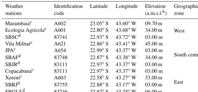
Table 1. Location of the surface andaupper-air weather observation stations.ba.m.s.l.: above mean sea level.
Weather Identification Latitude Longitude Elevation Geographic stations code (a.m.s.l.b) zone Marambaiac A602 23.05◦S 43.60◦W 09.70 m
West Ecologia Agricolac A601 22.80◦S 43.68◦W 34.00 m
SBSCd 83741 22.93◦S 43.72◦W 03.00 m Vila Militarc A621 22.86◦S 43.41◦W 45.00 m
South central JPAc A654 22.99◦S 43.37◦W 03.00 m
SBAFd 83748 22.87◦S 43.38◦W 34.00 m SBJRd 83111 22.97◦S 43.37◦W 03.00 m Copacabanac 83111 22.97◦S 43.37◦W 03.00 m
East Xeremc A603 22.58◦S 43.27◦W 33.00 m
SBRJd 83755 22.88◦S 43.17◦W 03.00 m SBGLa,d 83746 22.82◦S 43.25◦W 06.00 m
Source:cBrazilian National Institute of Meteorology anddMeteorology Network of the Brazilian Air Force Command.
Figure 2. The limited areas of G4 (resolution of 1 km), and the G5
and G6 innermost grids (resolution of 300 m).
et al. (1997). An external grid (GEXT) is set up in order to preprocess the data from the 0.5◦ Global Forecasting Sys-tem analyses (0.5◦-GFS; Kanamitsu, 1989), and to produce the first initial conditions (ICs) and lateral BCs at 3 h inter-vals for the outermost domain (G1), which has a horizontal resolution of 27 km. Relaxation on the values of the BCs is applied to a 5–10 grid-cell zone around the domain bound-ary, depending on the grid. In all simulations output data are produced at hourly intervals such that the data computed on any coarse grid are also employed as ICs and BCs at 3 h in-tervals for a subsequent fine-grid simulation in the one-way nested-grid domain. Namely, G1 produces data for G2, G2 for G3 and G3 for G4. Similarly, G4 produces data for both G5 and G6. In order to determine the horizontal resolutions for grids G2–G4 of the one-way nested-grid setup, we em-ploy a ratio of one grid size to the next equal to 3, all cen-tered with respect to the coarsest grid. The finest grids (G5
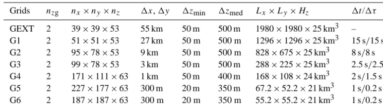
Table 2. Structure of the one-way nested numerical grids. Given the number of grid pointsnx,nyandnz, the physical domain size can be
calculated asLx×Ly×Hz, whereLx=(nx−3)1x,Ly=(ny−3)1y, andHz=(nz−3)1zmed.
Grids nzg nx×ny×nz 1x,1y 1zmin 1zmed Lx×Ly×Hz 1t/1τ
GEXT 2 39×39×53 55 km 50 m 500 m 1980×1980×25 km3 – G1 2 51×51×53 27 km 50 m 500 m 1296×1296×25 km3 15 s/15 s G2 2 95×78×53 9 km 50 m 500 m 828×675×25 km3 8 s/8 s G3 2 99×78×53 3 km 50 m 500 m 288×225×25 km3 2.5 s/2.5 s G4 2 171×111×63 1 km 50 m 400 m 168×108×24 km3 2 s/1.5 s G5 2 227×177×63 300 m 20 m 350 m 67.2×52.2×21 km3 1 s/0.2 s G6 2 187×187×63 300 m 20 m 350 m 55.2×55.2×21 km3 1 s/0.2 s
The ARPS original files of the 30 arc-sec (i.e., approx-imately 900 m) USGS (United States Geological Survey) topography database are preprocessed for grids G1–G3 in our simulations. Depending on the run configuration, the ARPS files for grids G4 and G6 are either preprocessed from the 30 arc-sec USGS (i.e., approximately 900 m) topography database or the 3 arc-sec SRTM (i.e., approximately 90 m) detailed and updated high-resolution topography database, which we have recently incorporated into ARPS. This in-corporation procedure required substantial modifications to the arpstrn.f90 source file of the original ARPS code, which can be downloaded directly from http://meteoro.cefet-rj.br/ leanderson/arps/ and run with the 3 arc-sec SRTM data on the ARPS model version 5.2.8. Details on how the arpstrn.f90 routine works can be seen in the file’s comment lines and also in Xue et al. (1995). In Fig. 3a and b it is possible to com-pare these two distinct databases processed for G5, where we can easily notice that the topographic details are much better reproduced by the 3 arc-sec SRTM data, especially in regions where the topography exceeds 800 m a.g.l. The high-resolution topography database allows a much more appro-priate definition of the surface boundary condition. Although a comparison between these databases for grid G6 is not shown, the east side of the G5 domain provides a good idea of what the topography maps look like for G6.
3.3 Vertical resolution and grid aspect ratio
ARPS incorporates a σ-coordinate system that follows the ground surface. The grids are stretched using a hyperbolic tangent function (Xue et al., 1995) that produces an aver-age spacing 1zmedand a domain heightHz equal to (nz− 3)1zmed, wherenzis the number of the vertical grid points. The smallest vertical spacing 1zmin used for each grid and the number of grid points below ground level nzg can be found in Table 2. To resolve the smallest structures of the atmosphere it is necessary to adopt high vertical resolutions, but the grid aspect ratio (1/1zmin, where 1=1x=1y) should not be extremely large to avoid numerical errors, especially in the horizontal gradients (Mahrer, 1984), and also to avoid distortion of the resolvable turbulent structures when runs are carried out in LES mode (Kravchenko et al.,
1996). Poulos (1999) and De Wekker (2002) have found that the aspect ratio of the grid should be small, especially for terrains with steep topography. Following the tutorials of Mahrer (1984), Kravchenko et al. (1996), Poulos (1999) and De Wekker (2002) and similar procedures adopted by Chow et al. (2006) we set up grids G1 and G2 with grid aspect ratios of 540 and 180 near the surface, respectively, to represent the scales in the atmosphere. These choices are adequate because the characteristic scales of the topography and the resolvable flow are large enough for the G1 and G2 domains, in addition to the fact that the 1.5-TKE parameterization scheme for the closure of the turbulent fluxes are used in both grids. Tests with high values of1zminfor grids G1 and G2 degraded the representation of the synoptic structures in comparison with the analysis of the synoptic charts, especially when we an-alyzed the mean atmospheric sea-level pressure fields. The same proportion was used for the G3 and G4 aspect ratios, since their1zminvalues are equal to the coarser grids. Par-ticularly, for the G5 and G6 grids, we avoided increasing the aspect ratio more than necessary and imposing a substantial decrease in the value of1zmin. Thus, we adopted an aspect ratio equal to 15, which results in a first level at 10 m a.g.l. and1zminequal to 20 m for the finest grids.
3.4 Land-use databases
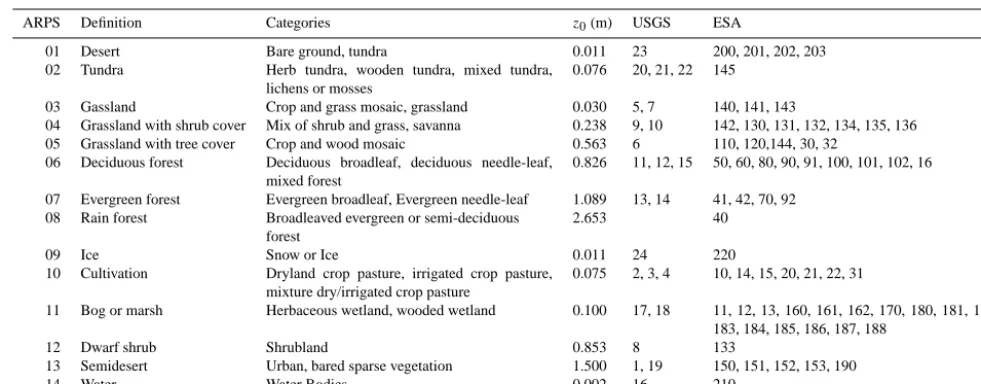
Table 3. Conversion of the original 30 arc-sec USGS and updated 10 arc-sec ESA categories of vegetation type to the USDA classification that
is adopted by ARPS. See tables in Xue et al. (1995) and Bicheron et al. (2008), and the user guide for more information on the vegetation-type categories.
ARPS Definition Categories z0(m) USGS ESA
01 Desert Bare ground, tundra 0.011 23 200, 201, 202, 203
02 Tundra Herb tundra, wooden tundra, mixed tundra, lichens or mosses
0.076 20, 21, 22 145
03 Gassland Crop and grass mosaic, grassland 0.030 5, 7 140, 141, 143
04 Grassland with shrub cover Mix of shrub and grass, savanna 0.238 9, 10 142, 130, 131, 132, 134, 135, 136 05 Grassland with tree cover Crop and wood mosaic 0.563 6 110, 120,144, 30, 32
06 Deciduous forest Deciduous broadleaf, deciduous needle-leaf, mixed forest
0.826 11, 12, 15 50, 60, 80, 90, 91, 100, 101, 102, 16
07 Evergreen forest Evergreen broadleaf, Evergreen needle-leaf 1.089 13, 14 41, 42, 70, 92 08 Rain forest Broadleaved evergreen or semi-deciduous
forest
2.653 40
09 Ice Snow or Ice 0.011 24 220
10 Cultivation Dryland crop pasture, irrigated crop pasture, mixture dry/irrigated crop pasture
0.075 2, 3, 4 10, 14, 15, 20, 21, 22, 31
11 Bog or marsh Herbaceous wetland, wooded wetland 0.100 17, 18 11, 12, 13, 160, 161, 162, 170, 180, 181, 182, 183, 184, 185, 186, 187, 188
12 Dwarf shrub Shrubland 0.853 8 133
13 Semidesert Urban, bared sparse vegetation 1.500 1, 19 150, 151, 152, 153, 190
14 Water Water Bodies 0.002 16 210
For the soil-type representation, the original 30 arc-sec USGS database files are processed and mapped into the grid categories set up in ARPS by selecting values from the nearest data points. For the vegetation-type representa-tion, original files of either the 30 arc-sec USGS database or the 10 arc-sec ESA (i.e., approximately 300 m) GlobCover-project database that we incorporated into ARPS are em-ployed, depending on the run. The incorporation of the veg-etation data into ARPS is carried out through the modifi-cations that we have introduced to the original arpssfc.f90 and arpssfclib.f90 source files. Particularly, we have devel-oped and added two new subroutines to the arpssfclib.f90 source file, referred to as GET_10S and MAPTY10S, which are similar to the GET_30S and MAPTY30S original sub-routines. The GET_10S subroutine reads 10 arc-sec or 300 m vegetation-type data resolution files from the ESA Glob-Cover project. The MAPTY10S subroutine transforms the 22 categories from 10 arc-sec vegetation-type data into the simpler 14 original vegetation-type USDA/ARPS categories and feed them into the model domain by choosing the data values at the nearest grid points. Beyond that, the setting of the surface-roughness (z0)map is processed by choosing val-ues associated to the vegetation-type classes, according to the same conversions shown in Table 3. Both the arpssfc.f90 and arpssfclib.f90 source files have been commented to explain the modifications and they can be downloaded directly from http://meteoro.cefet-rj.br/leanderson/arps/.
When the 30 arc-sec USGS vegetation-type database files are adopted in our runs, LAI is calculated from the 30 arc-sec USGS monthly NDVI database for herbaceous vegeta-tion and trees, respectively (Xue et al., 1995). The relavegeta-tion between the NDVI and LAI for herbaceous vegetation can be consulted in Asrar et al. (1984), and for trees in Nemani
Figure 3. Shaded topographic-elevation maps for G5, processed
with (a) 30 arc-sec USGS and (b) 3s-STRM databases.
Figure 4. Soil-type shaded maps for G5, processed with the 30
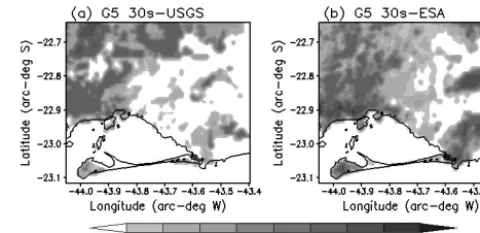
Figure 5. Vegetation-type shaded maps for G5, processed with (a)
30 arc-sec USGS and (b) 10 arc-sec ESA databases.
and Running (1989). Also, vegetation-fraction data from the 30 arc-sec National Environmental Satellite Data and Infor-mation Service (30 arc-sec NESDIS), supported by the Na-tional Oceanic and Atmospheric Administration (NOAA), are derived from the same NDVI data using the methodology suggested by Gutman and Ignotov (1998). However, when-ever the 10 arc-sec ESA vegetation-type database files are employed in our runs, LAI and vegetation fractions are di-rectly obtained from the 30 arc-sec ESA GlobCarbon project database, and little corrections on the mapped 30 arc-sec USGS soil-type data are needed near the coastlines of the water bodies, as illustrated by comparison in Fig. 4a and b for the G5 domain. We point out that we have developed the GETLAIGLOBCARBON and the GETFAPARGLOBCAR-BON subroutines and included them into the arpssfclib.f90 source file of the ARPS code. These routines are able to read the LAI and calculate the vegetation-fraction values, respec-tively, from the GlobCarbon project database and interpolate them into the model domain. In addition, we have also de-veloped the MAPTYLAIGLOBCARBON and MAPTYFA-PARGLOBCARBON subroutines to transform the 30 arc-sec ESA LAI and the FAPAR (Fraction of Absorbed Pho-tosynthetically Active Radiation) data into the simpler LAI and vegetation-fraction data and feed them into the model domain by choosing the data values at the nearest grid points. For an adequate reproduction of our results we also provide the namelist files – i.e., the arps.input files, and the SRTM and ESA databases at http://meteoro.cefet-rj.br/leanderson/ arps/ – in order to allow any setup we have used to run on all domain grids employed in this work.
Figure 5a and b highlight a comparison between the vegetation-type maps processed on G5 with the 30 arc-sec USGS and the 10 arc-sec ESA databases, respectively. It can be noticed that the 10 arc-sec ESA vegetation-type mosaic presents more detailed and smoothed areas than the 30 arc-sec USGS database. The analysis of Fig. 6a and b, which
Figure 6. Vegetation-cover-fraction shaded maps for G5, processed
with (a) 30 arc-sec USGS and (b) 30 arc-sec ESA databases.
illustrate a comparison of the vegetation-fraction maps on G5, indicates that the 30 arc-sec ESA vegetation fraction map presents a pattern that is in accordance with the pattern pre-sented by the 10 arc-sec ESA vegetation-type map. How-ever, the same does not exactly occur when we compare the 30 arc-sec USGS vegetation-fraction map to the 30 arc-sec USGS vegetation-type map. Therefore, we can safely con-clude that in this work it is better to use the ESA land-use database than the USGS database. The surface roughness maps are not shown here because they are closely related to vegetation-type information available in Table 3. Similarly, the LAI maps are also omitted because they are intimately re-lated to vegetation-type and vegetation-fraction information available on the maps in Figs. 5a and b and 6a and b.
Additionally, we use two soil layers with depths of 0.01 m and 1 m for the computation of the temperature and moisture balances according to the ARPS soil-vegetation model. The sea surface temperature (SST) and the soil skin temperature and moisture initial databases for the G1 grid are obtained from the 0.5◦-GFS analyses. For the subsequent grids, ini-tial values of these surface characteristics are obtained by numerical interpolation performed in each preceding grid. We also point out that, for all grids, we adopted the Colette et al. (2003) topography shading scheme, the Chou (1990) and Chou and Suarez (1994) short- and long-wave radiation schemes, the Kain and Fritsch (1990, 1993) microphysics scheme and the 1.5-TKE, Moeng and Wyngaard (1989) tur-bulence model. The Kessler (1969) and Lin et al. (1983) cu-mulus scheme is turned on only for the G1 and G2 synop-tic grids. Table 4 summarizes the differences adopted in our one-way nested-grid runs.
4 Results and discussion
Table 4. Summarized surface database configuration of the one-way nested numerical grids.
Grids Topography Soil type Vegetation type LAI Vegetation fraction G1–G3 30 arc-sec USGS 30 arc-sec USGS 30 arc-sec USGS 30 arc-sec USGS 30 arc-sec NESDIS G4–G6 CTL 30 arc-sec USGS 30 arc-sec USGS 30 arc-sec USGS 30 arc-sec USGS 30 arc-sec NESDIS
HR 3 arc-sec SRTM 30 arc-sec USGS 10 arc-sec ESA 30 arc-sec ESA 30 arc-sec ESA
boundary conditions, grid resolution and topographic and land-use databases, and to compare the results to surface and upper-air observational data for distinct days. We anticipate that, in the absence of frontal systems and depending on the positioning of SASA in the southeastern region of Brazil, the prevailing winds that blow in the region of interest are the re-sult of mesoscale and microscale mechanisms that occur as a function of the land–sea contrast, mountain–valley and land use.
4.1 Statistics indexes, meteograms and upper-air profiles
Analogously to Chow et al. (2006), Table 5 illustrates the mean errors (bias) and the root-mean-square errors (RMSE) computed for the potential temperatureθ, water-vapor mix-ing ratioqvand wind direction and speed for both runs of all periods. The results completely exclude the fast spin-up time of the indices and maintain only the computationally stable time results of the daily-cycle periods. The bias and RMSE are computed as follows:
bias= 1 N
N
X
i=1
ϕ0i, (1)
RMSE= v u u t
1 N
N
X
i=1
ϕi02, (2)
whereϕ0=ϕf−ϕorepresents the difference, or deviation, be-tween any forecasted and observed variable, andN is the to-tal number of verifications. For wind direction, a positive de-viation means that the simulated wind vector deviates clock-wise in relation to the observed wind vector. Because the largest possible error in wind direction is 180 arc-deg, the definition of the deviationϕ0needs to be changed according to
ϕ0=(ϕf−ϕo)
1− 360 |ϕf−ϕo|
,
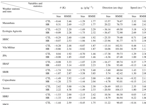
if |ϕf−ϕo|>180 arc-deg. (3) The analysis of the statistical indexes from Table 5 clearly summarizes that the HR-run results are much better than the CTL-run results. From the data displayed in Table 5, we see that the HR-run statistics are worse only in 6 out of the 22 statistics for potential temperature, and only in 2 out of
22 statistics for the wind speed. We consider these statisti-cal indexes to be very appealing. Specifistatisti-cally in the case of the wind speed, which is a very important quantity, the im-provement obtained in its calculation can be quantified by looking, for example, at the Marambaia and Ecologia Agrí-cola stations (located in the west zone). At Marambaia, Ta-ble 5 shows that there is a decrease of the bias from 2.32 to 1.66 m s−1, whereas at Ecologia Agrícola the decrease goes from 3.18 to 2.69 m s−1. Also, the RSME goes from 3.02 to 2.42 m s−1at Marambaia, and from 4.26 to 3.59 m s−1at Ecologia Agrícola. To support this line of reasoning, we cre-ated Table 6, which summarizes the statistics by classifying the stations into three zones as seen in Table 1. Table 6 shows that the wind speed results are better for the HR runs in the west and south-central zones, which adds up to 14 improve-ments out of 14 statistics.
From Tables 5 and 6, the statistical indexes for the po-tential temperature show significant improvement over the CTL run results when HR databases are employed. All cases are better for the HR runs in the east zone, and four out of six are better in the west zone. Considering all zones, only 6 cases out of 22 presented worse results with HR databases. Although we had four worse cases out of eight in the south-central zone, the calculated bias for both the CTL and the HR runs are small (less than 1.8 K for the west and south-central zones) compared to potential temperature values on the or-der of 300.0 K, which were calculated from observed, mea-sured values. In the east zone, where we had eight improve-ments out of eight statistics, the bias values are also small (in the range 1.5–2.6 K). This set of results indicates that ARPS, overall, is doing a good job in the prediction of the time and space variation of this quantity in the simulations, although the computed values tend to underestimate the observational data.
Table 5. Mean errors (bias) and RMSEs forθ,qv, wind direction and speed.
XX XX
XX XX
XX XX
XXX Weather stations
and runs
Variables and statistics
θ(K) qv(g kg−1) Direction (arc-deg) Speed (m s−1)
bias RMSE bias RMSE bias RMSE bias RMSE
Marambaia CTL −0.44 2.46 −1.29 1.77 13.57 76.67 2.32 3.02 HR 0.31 2.69 −1.27 1.77 20.22 76.75 1.66 2.42
Ecologia Agricola CTL −0.23 2.20 −1.69 2.29 −36.16 69.50 3.18 4.26 HR −0.09 2.28 −1.75 2.32 −36.47 72.90 2.69 3.59
SBSC CTL −0.29 2.60 −1.04 1.92 −25.35 79.48 0.71 2.60 HR −0.07 2.53 −1.06 1.94 −23.96 81.77 0.73 2.50
Vila Militar CTL −0.28 2.48 −0.87 1.87 −13.14 102.51 0.48 1.13 HR −0.86 2.34 −0.82 1.87 16.06 101.04 0.39 1.12
JPA CTL 0.04 1.92 −0.70 1.46 −17.38 59.73 1.29 2.36 HR −0.08 1.85 −0.65 1.46 −6.36 67.48 1.00 1.90
SBAF CTL −0.08 3.33 −1.07 2.29 −16.17 89.74 0.37 1.79 HR −0.83 3.14 −0.93 2.23 2.56 93.40 −0.13 1.68
SBJR CTL −1.74 3.01 −3.70 3.40 −3.60 60.04 1.43 2.31 HR −1.87 2.87 −3.58 3.85 5.74 62.42 1.30 2.08
Copacabana CTL −1.49 2.92 −1.43 2.00 −3.09 86.16 −0.32 2.13 HR −1.26 2.75 −1.44 2.04 −4.78 93.01 −0.15 2.43
Xerem CTL 2.62 5.00 −1.56 2.30 −26.49 105.11 2.35 3.68 HR 2.22 4.38 −1.49 2.33 −20.50 104.13 1.80 2.99
SBRJ CTL −1.53 2.00 −2.15 2.42 10.36 84.30 0.03 1.67 HR −1.33 1.89 −2.19 2.46 −8.79 84.94 0.22 1.86
SBGL CTL −1.44 2.59 −0.45 1.75 11.22 90.45 −0.16 1.66 HR −1.22 2.59 −0.48 1.77 14.54 84.50 −0.16 1.64
Table 6. Summary of the statistical indexes. Cases where the HR
run is worse than the CTL run, with respect to the total number of cases.
Variables zones θ Speed West 2/6 0/6 South central 4/8 0/8 East 0/8 2/8 Total 6/22 2/22
the calculation of the vapor-mixing ratio. Therefore, the sta-tistical indexes that compare the HR and CTL runs’ results should not be used directly to assess the advantage of the HR simulation over the CTL simulation. It is worth noting that we compared the observational and model results at the same height by extrapolating the ARPS results from the first grid point at 10 m down to 2 m.
In the case of the wind direction, large deviations between the ARPS runs are observed against observational data. De-spite the fact that the wind direction is probably the most
Figure 7. Time cross-section data of (a, b)θ(K), and (c, d) wind speed (m s−1)observed (closed circle) and simulated by G5 of the CTL (open triangle) and HR (open square) runs from 00:00 UTC 6 September to 00:00 UTC 8 September 2007 at Marambaia surface weather-observation station.
Figure 8. Time cross-section data of (a, b)θ(K), and (c, d) wind speed (m s−1)observed (closed circle) and simulated by G5 of the CTL (open triangle) and HR (open square) runs from 00:00 UTC 6 September to 00:00 UTC 8 September 2007 at Ecologia Agricola surface weather-observation station.
the model is unable to provide accurate lateral BC forcing for the finest grids, as discussed by Gohm et al. (2004). Regard-less of these issues, our results indicate that the scales mod-eled in the finest grids (G5 and G6), based on “Terra Incog-nita” (Wyngaard, 2004), are still accurate enough to provide encouraging results.
Figures 7–12 show the time cross-section data, or me-teograms, of potential temperature and wind speed that com-pare the simulated data from the CTL runs (open triangle) and the HR runs (open square) with the observational data (closed circle) for some surface weather stations where the
Figure 9. Time cross-section data of (a, b)θ(K), and (c, d) wind speed (m s−1)observed (closed circle) and simulated by G5 of the CTL (open triangle) and HR (open square) runs from 00:00 UTC 6 September to 00:00 UTC 8 September 2007 at SBSC surface weather-observation station.
Figure 10. Time cross-section data of (a, b) θ (K), and (c, d) wind speed (m s−1) observed (closed circle) and simulated by G5 of the CTL (open triangle) and HR (open square) runs from 00:00 UTC 6 February to 00:00 UTC 8 February 2009 at SBAF sur-face weather-observation station.
Figure 11. Time cross-section data of (a, b)θ(K), and (c, d) wind speed (m s−1)observed (closed circle) and simulated by G5 of the CTL (open triangle) and HR (open square) runs from 00:00 UTC 6 February to 00:00 UTC 8 February 2009 at JPA surface weather-observation station.
can be noticed at almost all times, mainly for the HR run (Fig. 7c, d). We also note the occurrence of large speed val-ues in the periods 18:00–21:00 UTC 6 September and 15:00– 17:00 UTC 7 September 2007, which are associated with the sea breeze coming from the Atlantic Ocean. The simulation results show just a slight discrepancy with respect to this be-havior on the second day, since ARPS does not compute ad-equately the speed decrease from 18:00 UTC on, showing a possible influence of the synoptic forcing in the model-ing process of the ABL and hidmodel-ing the real effect of the sea breeze coming from the Atlantic Ocean.
The observed daily cycles for the potential temperature are also represented qualitatively well by the simulation for both runs at the Ecologia Agricola station (Fig. 8a, b). The com-puted results for the HR run present better agreement with the observational data than the CTL run between 08:00 and 14:00 UTC for both days, just when the convective mixed layer is in development. The results illustrated by time cross section of the wind speed computed from the HR run present better agreement with the observational data than the CTL run, although the results show a systematic trend to overesti-mate the wind speed (Fig. 8c, d). The Ecologia Agricola sta-tion is posista-tioned relatively far from Sepetiba Bay (Fig. 1), in a direction transverse to the coastline. Thus, the sea breeze is sometimes the driving force of the wind speed and direction, as it probably occurred on 7 September 2007. Based on these results and similar results obtained by Chow et al. (2006) for other regions, we infer that the poor representation of the 30 arc-sec USGS soil type can greatly influence the results of the simulation, in spite of the best representation of the topography and vegetation-type provided in the HR run.
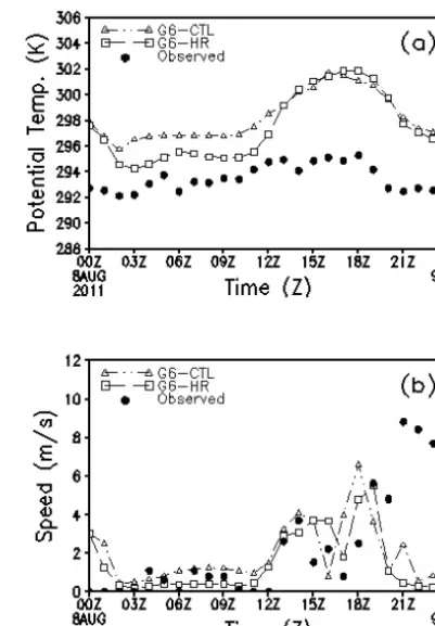
Figure 12. Time cross-section data of (a) θ (K), and (b) wind speed (m s−1)observed (closed circle) and simulated by G6 of the CTL (open triangle) and HR (open square) runs from 00:00 UTC 8 August to 00:00 UTC 9 August 2011 at Xerem surface weather-observation station.
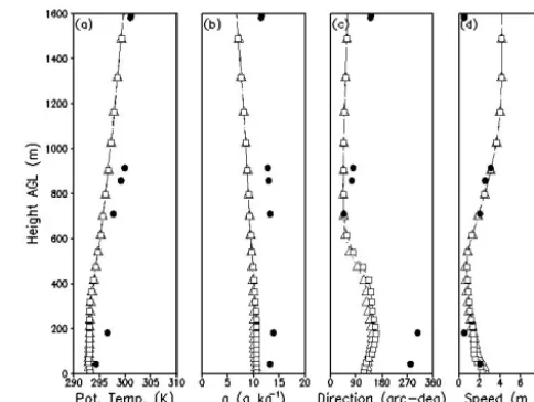
Figure 13. Vertical data profiles of (a)θ (K), (b)qv(g kg−1), (c)
wind direction (arc-deg) and (d) speed (m s−1) observed (closed circle) and simulated by G6 of the CTL (open triangle) and HR (open square) runs for 12:00 UTC 6 September 2007 at SBGL upper-air weather-observation station.
represent the wind speed and direction behavior at the SBSC station. Even with the good performance of the computed daily wind-speed cycle for the HR run on the second day an-alyzed (Fig. 9d), we highlight that there are combined effects due the synoptic scale and the sea breeze coming from the Atlantic Ocean and Sepetiba Bay. The low resolution of the soil-type database associated to soil temperature and mois-ture initialization data may be affecting the modeled results in this region too.
The daily cycles for the potential temperature computed at the SBAF station (Fig. 10a, b) also presented successful results on the second period (Feb/2009) – i.e., in the period from 00:00 UTC 6 February to 00:00 UTC 8 Feburary 2009 – as observed for other stations. The CTL run performs better than the HR run only at some periods of the day, showing in a convincing way that the HR run presents important results for a region characterized by valley–mountain effects (see the eastern side of Fig. 3a and b). We note that the ARPS results tend to overestimate the observational data for the potential temperature at night, dawn and early morning (about 21:00– 09:00 UTC), and tend to underestimate them in the period morning–afternoon (about 11:00–15:00 UTC). In general, the calculated wind speed values are lower than the observa-tional data between 06:00 and 15:00 UTC 6 Feburary 2009 and between 00:00 and 12:00 UTC 7 Feburary 2009, mainly due to the SBAF location, where the wind direction can be driven by a sum of two factors: the weak catabatic winds from the Pedra Branca (see the mountain in the northeast of Fig. 3a and b) and Tijuca massifs (see the mountain in the southeast of Fig. 3a and b), and the weak land breeze. At the same time intervals, we note from the wind direction me-teograms (not shown) that the wind blows (with variation)
Figure 14. Vertical data profiles of (a)θ(K), (b)qv(g kg−1), (c)
wind direction (arc-deg) and (d) speed (m s−1)observed (closed circle) and simulated by G6 of the CTL (open triangle) and HR (open square) runs for 12:00 UTC 7 September 2007 at SBGL upper-air weather station.
from NNE (land and mountain breeze) and SSE (mountain breeze). For both days (Fig. 10a, b), the flow accelerates slightly when the wind blows from the S and SE (not shown) in the period 15:00–21:00 UTC, approximately, suggesting the occurrence of a canalized jet due to the sea-breeze ef-fect from the Atlantic Ocean. In general, the HR run over-comes the CTL run for most of the time when we compare the wind speed results to the observational data, as illustrated in Fig. 10c and d.
Figure 15. Horizontal cross section of the difference of potential temperature (K – shaded areas) between runs for the G5 domain, calculated
asθ(HR) –θ(CTL), for (a) 14:00, (b) 15:00, (c) 16:00 and (d) 17:00 UTC, 7 September 2007.
Satisfactory results for the daily cycle of the potential tem-perature in the third period (August 2011) – i.e., between 00:00 UTC 8 August and 00:00 UTC 9 August 2011 – can be seen in Fig. 12a and b for the Xerem station. However, the ARPS results for the potential temperature overestimate a little the potential temperature obtained with the observa-tional data at all times. Small discrepancies between the CTL and the HR runs are detected after 13:00 UTC; however the HR run overcomes clearly the CTL run between 02:00 and 12:00 UTC. The main cause of the discrepancies found in the wind direction (not shown) is the occurrence of calm winds, which reach a maximum of 9 m s−1 at 21:00 UTC. We highlight the occurrence of calm winds between 00:00 and 12:00 UTC and moderate winds in the afternoon and night (between 13:00 UTC 8 August and 00:00 UTC 9 Au-gust 2011), just when the sea-breeze flow from the Atlantic Ocean is completely developed in conjunction with anabatic wind effects from Tijuca Massif (Fig. 12c, d). In general, wind speed values computed by the HR run are a little bet-ter than the CTL run when compared to observational data. The discrepancy is larger after 21:00 UTC. But in such situ-ations, when the wind speed is very calm, the turbulence pa-rameterization schemes typically show considerable difficul-ties in modeling the flow near the ground under the referred-to conditions; i.e., calm winds, intermittent flow and, nor-mally, when mesoscale models are downscaling to the LES domains. However, it is important to point out that the re-sults obtained from the simulations reproduce qualitatively the observed maximum wind speed in the afternoon and the minimum wind speed in the morning.
occurrence of low wind speed near the ABL and higher wind speed up to 1600 m a.g.l.
4.2 Difference of potential temperature fields
In order to show the spatial discrepancies between the HR and the CTL runs on the G5 domain, we present the horizon-tal cross section of the difference of potential temperature between the two runs, defined as θ(HR) –θ(CTL), for the period from 14:00 to 17:00 UTC, 7 September 2007, as illus-trated in Fig. 15a–d. This figure highlights the areas where there are visible discrepancies between both runs. These re-sults also indicate that changes alone on the vegetation type and not merely on the soil type provide meaningful differ-ences on the air flow, as we can see from the contrast between the continent and the sea. We inserted a dashed line in each figure to indicate the vertical cross section which we con-sidered in the analysis of the sea-breeze front based on the TKE distribution that we present in Sect. 4.3. At 14:00 UTC (11:00 local time – LT), we can clearly observe that the ma-jor discrepancies are on the western side and over the water bodies, mainly in the vicinity of a water reservoir located in the continent. Overall, the potential temperature values of the HR run tend to be higher than those of the CTL, except around the entrance of Sepetiba Bay, where a colder air par-cel due to the HR run appears (Fig. 15a). In this case, the re-sults for the HR run present an accentuated differential heat-ing between the sea and the continent, which is able to turn on an efficient thermodynamic trigger to start the sea–land breeze mechanism. Thus, it is possible that the vegetation-type database changes the heat and water-vapor fluxes in order to represent more adequately the local circulation. At 15:00 UTC (Fig. 15b) the discrepancy increases slightly and the cool air parcel moves from the southeast to the northwest, indicating that the sea-breeze front penetrates perpendicu-larly into the continent with respect to the grid’s east-side shoreline (approximately between −43.60 and−43.40 arc-deg west longitude). During this motion, the breeze does not feel the change in direction that the Sepetiba Bay shoreline presents after−43.60 arc-deg west longitude, approximately, which the dashed line crosses. Likewise, this behavior indi-cates that the soil-type database that represents this change in direction of the Sepetiba Bay shoreline is not influenc-ing the flow enough to capture the wind direction suitably in this area. At 16:00 and 17:00 UTC (Fig. 15c, d) we note the same discrepancy areas between the runs as seen in the previous hour, but the potential temperature difference val-ues are smaller. The cool air parcel moves towards the grid’s west side at 16:00 UTC (Fig. 15c), and practically disappears at 17:00 UTC (Fig. 15d). This behavior shows the impor-tance of increasing the density of surface-weather observa-tion staobserva-tions at MARJ in order to evaluate whether the phys-ical trend captured with the high-resolution ARPS modeling is in agreement with the sea-breeze front advance analyzed.
4.3 Vertical-latitudinal cross-section analysis
Figure 16a–d illustrate the vertical-latitudinal cross-section distribution of TKE, potential temperature and meridional-vertical wind vector components only for the HR run, com-puted at−43.60 arc-deg west longitude (Marambaia longi-tude location) in the period 14:00–17:00 UTC, 7 Septem-ber 2007, since the HR results are better than the CTL re-sults. The scale goes from 0 to 1000 m a.g.l. and the color scale ranges between 0.05 and 3.0 m2s−2. The dashed line which crosses each panel in Fig. 16a–d indicates where the land and sea cross sections are located in order to support our analysis. The calculations were performed in this period because we are interested in highlighting the TKE distribu-tion close to the sea-breeze front indicated by the meteogram analysis from the Marambaia station (Fig. 7). One can see that the TKE distribution in the northern part of the conti-nental region (between−22.90 and−22.65 arc-deg south lat-itude) may be associated, at all times, to the near-surface ver-tical shear and buoyancy effects caused mainly by the moun-tain waves (see topographic elevation maps in Fig. 3a, b), as also suggested by the numerical results for the wind ve-locity vector and vertical potential temperature gradient. In this region of the cross section, the TKE intensity presents higher values at 15:00 and 16:00 UTC (see Fig. 16b and c) due to the higher temperatures and wind shear computed. At 14:00 UTC (Fig. 16a), a stably stratified ABL occurs over the ocean region and near the coastline (between−23.11 and −23.00 arc-deg south latitude), and one can see a northerly wind component blowing along the vertical-latitudinal cross section beyond 200 m a.g.l. Below this level, on the surface layer, there is evidence that a southerly wind component starts the sea-breeze flow, which is associated with a weak horizontal gradient and a relative intense TKE distribution at the sea-breeze front near the coastline.
Figure 16. Vertical-latitudinal cross section of TKE (m2s−2– shaded areas), potential temperature (K – solid line) and meridional-vertical wind vector components (m s−1– vectors) up to 1.0 km a.g.l. at−43.60 arc-deg west longitude (Marambaia longitude location). Values calculated on G5 for the HR run at (a) 14:00, (b) 15:00, (c) 16:00 and (d) 17:00 UTC, 7 September 2007.
(see also Fig. 8). In the HR run results, a return circula-tion (the anti-sea breeze) of about 5 m s−1 brings warmer air back to the sea, which descends towards the sea surface and closes the circulation circuit. We can also note that, at 14:00 and 15:00 UTC (Fig. 16a, b), the speed of the follow-ing sea breeze is a little faster than the speed of the sea-breeze front, and a light wave propagates upstream of the sea-breeze front as the southerly flow component collides with the adverse northerly flow component. When the fol-lowing sea-breeze reaches the front, convergence results in a “head-shaped” updraft, as also seen by Reible et al. (1993) and Bastin and Drobinski (2006). This “head” is a zone of in-tense mixing, which is supported by the significant values of the TKE shown in Fig. 16b. We also observe that the highest TKE values occur in the mesoscale cold-front region around 450 m a.g.l. and near the ground surface. The vertical motion of the air is evident in the HR run at 14:00–15:00 UTC (see Fig. 16a and b). The maximum depth of the sea-breeze is ob-served to be at approximately 300 m a.g.l. at all times. After 17:00 UTC the magnitude of the updraft decreases quickly, as well as its vertical extent, and the TKE intensity decreases slowly with time near the surface. Also, the northerly com-ponent of the upper-level wind strengthens, whereas the TKE decreases and remains confined near the surface, where some shear appears.
5 Summary and conclusions
Numerical simulations of the ABL flow are strongly in-fluenced by several factors; namely, the parametric mod-els adopted in the boundary value problem that represents the physical situation, the numerical methods applied to solve the conservation equations, the numerical-grid scheme, and the boundary conditions related to the synoptic forcing and surface databases. In order to reduce the influence of these factors, we incorporate into ARPS the 3 arc-sec SRTM topographic database, the 10 arc-sec ESA vegetation-type database and the 30 arc-sec ESA LAI and FAPAR databases, which are preprocessed by subroutines we developed for the ARPS architecture. These subroutines are available to the scientific community. The numerical simulations are carried out in the LES mode for three time periods, running on six one-way nested grids that are setup separately, such that dif-ferent vertical resolutions and parameterizations are chosen for each scale being modeled.
potential temperature and wind speed results observed for the HR run present significantly lower errors than for the CTL run, but do not lead necessarily to better simulation results in all variables. This fact indicates that additional improvement will depend on other factors, such as the local surface charac-terization, the turbulence closure and other microphysics pa-rameterizations associated to the numerical mesoscale model employed.
For the cases we studied, our simulations showed that there is no significant difference between the bias values cal-culated from the HR and the CTL runs for the vapor-mixing ratio. Although this result may inconclusively support that the use of HR databases over low-resolution databases is ad-vantageous, we point out that the bias values we obtained are small compared to the observation data. In the case of the wind direction, which is probably the most difficult quantity to accurately forecast with any model, large deviations be-tween the ARPS runs were observed against observational data. However, the HR runs show significant improvement over the CTL run at the SBAF and JPA stations. From a statistical point of view, the HR flow model performs very well in the prediction of the time and space variation of these quantities using ARPS simulations.
From a closer look at the results obtained for some spe-cific surface stations, we infer that, at the SBAF station for example, both runs forecasted well the canalized jet triggered by the sea-breeze effect. However, at the SBSC and Xerem stations, the wind speed presents increased discrepancies in some periods of time due to the occurrence of calm winds in the simulation. As Hanna and Yang (2001) pointed out, the turbulence parameterization schemes typically have dif-ficulties in modeling the flow near the ground under condi-tions of calm, intermittent flow and when mesoscale models are downscaling to LES domains. Equivalent statistical re-sults and conclusions were obtained by Chow et al. (2006), demonstrating again the difficulties in modeling the wind field. Some clear discrepancies were observed, mainly at the moments when a flow transition occurs to form the sea breeze. However, the remarkable TKE distribution on the sea-breeze front shows a pattern very similar to the one found by Bastin and Drobinski (2006), which is evidence of a con-sistent physical behavior. In accordance with the literature, our results indicate that an improved representation of the properties and characteristics of the land use can dramati-cally influence the calculation of the momentum, heat and moisture fluxes between the surface and the atmosphere, and may significantly affect the calculation of the meteorologi-cal field quantities. This suggests a need for improving our soil-type databases, and soil moisture and temperature ini-tializations.
Acknowledgements. The authors acknowledge the collaboration
of Fotini Katapodes Chow, from the University of California at Berkeley, for valuable suggestions; Vasileios Kalogirou, from ESA/ESRIN, for invaluable support with the ESA database; Kevin W. Thomas, Ming Xue and Yunheng Wang, from the Center for Analysis Prediction of Storms, for technical support with ARPS. The authors would also like to acknowledge the Brazilian National Institute of Meteorology and Meteorology Network of the Brazilian Air Force Command, for making available the observational surface data, in addition to CNPq, CAPES and FAPERJ for their financial support.
Edited by: H. Garny
References
Arino, O., Ranera, F., Plummer, S., and Borstlap, G.: GlobCarbon product description, 28 pp., available at: http://dup.esrin.esa.it/ files/p43/GLBC_ESA_PDMv4.2.pdf (last access: 21 November 2013), 2008.
Asrar, G., Fuchs, M., Kanemasu, E. T., and Hatfield, J. L.: Estimat-ing absorbed photosynthetic radiation and leaf area index from spectral reflectance in wheat, Agron. J., 76, 300–306, 1984. Bastin, B. S. and Drobinsky, P.: Sea-breeze-induced mass transport
over complex terrain in south-eastern France: A case-study, Q. J. R. Meteorol. Soc., 132, 405–423, 2006.
Beljaars, A. C. M., Viterbo, P., Betts, A., and Miller, M. J.: The anomalous rainfall over the United States during July 1993: Sen-sitivity to land surface parameterization and soil moisture anoma-lies, Mon. Weather Rev., 124, 362–384, 1996.
Bicheron, P., Defourny, P., Brockmann, C., Schouten, L., Van-cutsem, C., Huc, M., Bontemps, S., Leroy, M., Achard, F., Herold, M., Ranera, F., and Arino, O.: GLOBCOVER Prod-ucts description and Validation Report, available at: http: //due.esrin.esa.int/globcover/LandCover_V2.2/GLOBCOVER_ Products_Description_Validation_Report_I2.1.pdf (last access: 21 November 2013), 2008.
Black, T. L.: The new NMC mesoscale eta model: Description and forecast examples, Weather Forecast, 9, 265–278, 1994. Bubnová, R., Horányi, A., and Malardel, S.: International project
ARPEGE/ALADIN, in: EWGLAM, Newsletter 22, de Belgique IRM, 117–130, 1993.
Businger, J. A., Wyngaard, J. C., Izumi, Y., and Bradley, E. F.: Flux-profile relationships in the atmospheric surface layer, J. Atmos. Sci., 28, 181–189, 1971.
Castro, F. A., Palma, J. M. L. M., and Silva Lopes, A.: Simulations of the Askervein flow. Part I: Reynolds averaged Navier-Stokes equations (k –εTurbulence Model), Bound.-Lay. Meteorol., 107, 501–530, 2003.
Chen, Y., Ludwig, F. L., and Street, R. L.: Stably-stratified flows near a notched, transverse ridge across the Salt Lake Valley, J. Appl. Meteorol., 43, 1308–1328, 2004.
Chou, M.-D.: Paramemterization for the absorption of solar radia-tion by O2and CO2with application to climate studies, J.
Cli-mate, 3, 209–217, 1990.
In-formation, 800 Elkridge Landing Road, Linthicum Heights, MD 21090-2934, 85 pp., 1994.
Chow, F. K.: Subfilter-scale turbulence modeling for large-eddy simulation of the atmospheric boundary layer over complex terrain, Ph.D. dissertation, Stanford University, Environmental Fluid Mechanics and Hydrology, Department of Civil and En-vironmental Engineering, California, USA, 339 pp., 2004. Chow, F. K. and Street, R. L.: Evalution of turbulence closure
mod-els for large-eddy simulation over complex terrain: flow over Askervein Hill, J. Appl. Meteorol. Clim., 48, 1050–1065, 2009. Chow, F. K., Street, R. L., Xue, M., and Ferziger, J. H.: Explicit
filtering and reconstruction turbulence modeling for large-eddy simulation of neutral boundary layer flow, J. Atmos. Sci., 62, 2058–2077, 2005.
Chow, F. K., Weigel, A. P., Street, R. L., Rotach, M. W., and Xue, M.: High-resolution large-eddy simulations of flow in a steep Alpine valley. Part I: Methodology, verification, and sensitivity experiments, J. Appl. Meteorol. Clim., 45, 63–86, 2006. Colette, A., Chow, F. K., and Street, R. L.: A numerical study of
inversion-layer breakup and the effects of topographic shading in idealized valleys, J. Appl. Meteorol., 42, 1255–1272, 2003. Deardorff, J. W.: Parameterization of the planetary boundary layer
for use in general circulation models, Mon. Weather Rev., 100, 93–106, 1972.
De Wekker, D. G. S., Fast, J. D., Rotach, M. W., and Zhong, S.: The performance of RAMS in representing the convective boundary layer structure in a very steep valley, Environ. Fluid. Mech., 5, 35–62, 2005.
De Wekker, S. F. J: Structure and morphology of the convective boundary layer in mountainous terrain, Ph.D. dissertation, Uni-versity of British, Columbia, 191 pp., 2002.
Dudhia, J., Gill, D., Guo, Y. R., Manning, K., Wang, W., and Chiszar, J.: PSU/NCAR Mesoscale Modeling System, Tuto-rial Class Notes and User’s Guide: MM5 Modeling Sys-tem Version-3, available at: http://www.mmm.ucar.edu/mm5/ documents/tutorial-v3-notes-pdf/tutorial.cover.pdf (last access: 25 November 2009), 256 pp., 2005.
Eyndt, T. O., Serruys, P., Borstlap, G., Tansey, K., and Benedetti, R.: GlobCarbon demonstration products and qualification report, European Space Agency, 161 pp., available at: http://dup.esrin. esa.it/prjs/Results/131-176-149-30_200936105837.pdf (last ac-cess: 21 November 2013), 2007.
Farr, T. G. and Kobrick, M.: Shuttle Radar Topography Mission pro-duces a wealth of data, EOS-Trans. Amer. Geophys. Union, 81, 583–585, 2000.
Gasperoni, N. A., Xue, M., Palmer, R. D., and Gao, J.: Sensitivity of convective initiation prediction to near-surface moisture when assimilating radar refractivity: Impact tests using OSSEs, J. At-mos. Ocean. Tech., 30, 2281–2302, 2013.
Gohm, A., Zäangl, G., and Mayr, G. J.: South foehn in the Wipp Valley on 24 October 1999 (MAP IOP 10): Verification of high-resolution numerical simulations with observations, Mon. Weather Rev., 132, 78–102, 2004.
Grell, G. A., Dudhia, J., and Stauffer, D. R.: A description of the fifth generation Penn State/NCAR mesoscale model, NCAR Tech. Note, NCAR/TN-398+STR, 117 pp., available at: http: //www.mmm.ucar.edu/mm5/documents/mm5-desc-pdf/ (last ac-cess: 20 January 2008), 1993.
Grell, G. A., Emeis, S., Stockwell, W. R., Schoenemeyer, T., Forkel, R., Michalakes, J., Knoche, R., and Seidl, W.: Application of a multi-scale, coupled MM5/chemistry model to the complex terrain of the VOTALP valley campaign, Atmos. Environ., 34, 1435–1453, 2000.
Grøn˙as, S. and Sandvik, A. D.: Numerical simulations of local winds over steep orography in the storm over north Norway on October 12, 1996, J. Geophys. Res., 104, 9107–9120, 1999. Gutman, G. and Ignatov, A.: The derivation of the green vegetation
fraction from NOAA/AVHRR data for use in numerical weather prediction models, Int. J. Remote Sens., 19, 1533–1543, 1998. Hanna, S. R. and Yang, R. X: Evaluations of mesoscale models
sim-ulations of near-surface winds, temperature gradients, and mix-ing depths, J. Appl. Meteorol., 40, 1095–1104, 2001.
Horányi, A., Ihász, I., and Radnóti, G.: ARPEGE/ALADIN: A nu-merical weather prediction model for Central-Europe with the participation of the Hungarian Meteorological Service, Idöjárás, 100, 277–300, 1996.
Kain, J. S. and Fritsch, J. M.: A one-dimensional entrain-ing/detraining plume model and its application in convective pa-rameterization, J. Atmos. Sci., 47, 2784–2802, 1990.
Kain, J. S. and Fritsch, J. M.: Convective parameterization for mesoscale models: The Kain-Fritsch scheme. The Represen-tation of Cumulus Convection in Numerical Models, Meteor. Monogr., 24, 165–170, 1993.
Kanamitsu, M.: Description of the NMC global data assimilation and forecast system, Weather Forecast., 4, 335–342, 1989. Kessler, E.: On the distribution and continuity of water substance in
atmospheric circulation, Meteor. Mon., 10, 1–84, 1969. Kravchenko, A. G., Moin, P., and Moser, R.: Zonal embedded grids
for numerical simulations of wall-bounded turbulent flows, J. Comput. Phys., 127, 412–423, 1996.
Lafore, J. P., Stein, J., Asencio, N., Bougeault, P., Ducrocq, V., Duron, J., Fischer, C., Héreil, P., Mascart, P., Masson, V., Pinty, J. P., Redelsperger, J. L., Richard, E., and Vilà-Guerau de Arellano, J.: The Meso-NH Atmospheric Simulation System. Part I: adi-abatic formulation and control simulations, Ann. Geophys., 16, 90–109, doi:10.1007/s00585-997-0090-6, 1998.
Lin, Y.–L., Farley, R. D., and Orville, H. D.: Bulk parameterization of the snow field in a cloud model, J. Clim. Appl. Meteorol., 22, 1065–1092, 1983.
Lopes, A. S., Palma, J. M. L. M., and Castro, F. A.: Simulation of the Askervein flow. Part 2: Large-eddy simulations, Bound.-Lay. Meteorol., 125, 85–108, 2007.
Lu, R. and Turco, R. P.: Air pollutant transport in a coastal environ-ment – II. three-dimensional simulations over Los Angeles basin, Atmos. Environ., 29, 1499–1518, 1995.
Lucena, A. J., Filho, O. C. R., França, J. R. A., Peres, L. F., and Xavier, L. N. R.: Urban climate and clues of heat island events in the metropolitan area of Rio de Janeiro, Theor. Appl. Climatol., 111, 497–511, doi:10.1007/s00704-012-0668-0, 2012.
Mahrer, Y.: An improved numerical approximation of the horizontal gradients in a terrain-following coordinate system, Mon. Weather Rev., 112, 918–922, 1984.
Michioka, T. and Chow, F. K.: High-Resolution Large-Eddy Simu-lations of scalar transport in Atmospheric Boundary Layer flow over complex terrain, J. Appl. Meteorol. Clim., 47, 3150–3169, 2008.
Moeng, C. -H. and Wyngaard, J. C.: Evaluation of turbulent trans-port and dissipation closures in second-order modeling, J. At-mos. Sci., 46, 2311–2330, 1989.
Nemani, R. and Running, S. W.: Testing a theoretical climate-soil-leaf area hydrologic equilibrium of forests using satellite data and ecosystem simulation, Agr. Forest. Meteorol., 44, 245–260, 1989.
Noilhan, J. and Planton, S.: A simple parameterization of land sur-face processes for meteorological models, Mon. Weather Rev., 117, 536–549, 1989.
Pitman, A. J.: The evolution of, and revolution in, land surface schemes designed for climate models, Int. J. Climatol., 23, 479– 510, 2003.
Pleim, J. E. and Xiu, A.: Development and testing of a surface flux and planetary boundary layer model for application in mesoscale models, J. Appl. Meteorol., 34, 16–32, 1995.
Pope, S. B.: Turbulent Flows. Cambridge University Press, Cam-bridge, UK, 2000.
Poulos, G.: The interaction of katabatic winds and mountain waves, Ph.D. dissertation, Colorado State University, 300 pp. USA, 1999.
Radnóti, G., Ajjaji, R., Bubnová, R., Caian, M., Cordoneanu, E., Von Der Emde, K., Gril, J. D., Hoffman, J., Horányi, A., Issara, S., Ivanovici, V., Janousek, M., Joly, A., Le Moigne, P., and Malardel, S.: The spectral limited area model ARPEGE/ALADIN, Proceedings of Workshop on limited-area and variable-resolution models, (Beijing, 23–27 Oct 1995) WWRP-PWPR Report Series 7, WMO-TD-699, Geneva (Switzerland), 111–118, 1995.
Reible, D. D., Simpson, J. E., and Linden, P. F.: The sea breeze and gravity current frontogenesis, Q. J. Roy. Meteor. Soc., 119, 1–16, 1993.
Revell, M. J., Purnell, D., and Lauren, M. K.: Requirements for large-eddy simulation of surface wind gusts in a mountain val-ley, Bound.-Lay. Meteorol., 80, 333–353, 1996.
Richter, I., Mechoso, C. R., and Robertson, A. W.: What determines the position and intensity of the South Atlantic Anticyclone in austral winter? – An AGCM study, J. Climate, 21, 214–229, 2008.
Rotach, M. W., Calanca, P., Graziani, G., Gurtz, J., Steyn, D. G., Vogt, R., Andretta, M., Christen, A., Cieslik, S., Conolly, R., De Wekker, S., Galmarini, S., Kadygrov, E. N., Kadygrov, V., Miller, E., Neininger, B., Rucker, M., Van Gorsel, E., Weber, H., Weiss, A., and Zappa, M.: Turbulence structure and exchange processes in an Alpine valley: The Riviera project, B. Am. Meteorol. Soc., 85, 1367–1385, 2004.
Skamarock, W. C., Klemp, J. B., and Dudhia, J.: Prototypes for the WRF (Weather Research and Forecast) model, Preprints, Ninth Conf. on Mesoscale Processes, Fort Lauderdale, FL, Amer. Me-teor. Soc., CD-ROM, J1.5, 2001.
Skamarock, W. C., Klemp, J. B., Dudhia, J., Gill, D. O., Barker, D. M., Wang, W., and Powers, J. G.: A description of the Ad-vanced Research WRF Version 2, NCAR Tech. Note NCAR/TN-468&STR, 88 pp., 2005.
Taylor, P. A. and Teunissen, H. W.: The Askervein Hill Project: Re-port on the September/October 1983 main field experiment, In-ternal Report MSRB-84-6, Downsview, Ontario, Canada, 1985. Taylor, P. A. and Teunissen, H. W.: The Askervein Hill Project:
Overview and background data, Bound.-Lay. Meteorol., 39, 15– 39, 1987.
Viterbo, P. and Betts, A. K.: Impact of the ECMWF reanalysis soil water on forecasts of the July 1993 Mississippi flood, J. Geophys. Res.-Atmos., 104, 19361–19366, 1999.
Walko, R. L., Tremback, C. J., and Hertenstein, R. F. A.: RAMS: The Regional Atmospheric Modeling System, User’s guide, ver-sion 3b, ASTER Diviver-sion, Misver-sion Research, Inc., Rep., 117 pp., available at: http://www.atmet.com/html/docs/rams/user_3b. ps (last access: 21 November 2013), 1995.
Warner, T. T., Peterson, R. A., and Treadon, R. E.: A tutorial on lat-eral boundary conditions as a basic and potentially serious limita-tion to regional numerical weather prediclimita-tion, B. Am. Meteorol. Soc., 78, 2599–2617, 1997.
Weigel, A. P., Chow, F. K., and Rotach, M. W.: The effect of moun-tainous topography on moisture exchange between the “surface” and the free atmosphere, Bound.-Lay. Meteorol., 125, 227–244, 2006.
Weigel, A. P., Chow, F. K., and Rotach, M. W.: On the nature of turbulent kinetic energy in a steep and narrow Alpine valley, Bound.-Lay. Meteorol., 123, 177–199, 2007.
Wyngaard, J. C.: Toward numerical modeling in the “Terra Incog-nita”, J. Atmos. Sci., 61, 1816–1826, 2004.
Xue, M., Droegemieer, K. K., and Wong, V.: The Advanced Re-gional Prediction System (ARPS): A multi-scale nonhydrostatic atmospheric simulation and prediction model. Part I: Model dy-namics and verification, Meteorol. Atmos. Phys., 75, 161–193, 2000.
Xue, M., Droegemieer, K. K., Wong, V., Shapiro, A., and Brewster, K.: ARPS Version 4.0 User’s Guide, 380 pp., available at: http: //www.caps.ou.edu/ARPS/arpsdoc.html (last access: 10 January 2007), 1995.
Xue, M., Droegemieer, K. K., Wong, V., Shapiro, A., Brewster, K., Carr, F., Weber, D., Liu, Y., and Wang, D.: The Advanced Re-gional Prediction System (ARPS) – A multi-scale nonhydrostatic atmospheric simulation and prediction model. Part II: Model Physics and Applications, Meteorol. Atmos. Phys., 76, 143–165, 2001.
Zängl, G., Chimani, B., and Haberli, C.: Numerical simulations of the foehn in the Rhine Valley on 24 October 1999 (MAP IOP 10), Mon. Weather Rev., 132, 368–389, 2004.
Zeri, M., Oliveira-Júnior, J. F. and Lyra, G. B.: Spatiotemporal anal-ysis of particulate matter, sulfur dioxide and carbon monoxide concentrations over the city of Rio de Janeiro, Brazil, Meteo-rol. Atmos. Phys., 113, 139–152, doi:10.1007/s00703-011-0153-9, 2011.